Exact ground state for a class of matrix Hamiltonian models: quantum phase transition and universality in the thermodynamic limit

Abstract

By using a recently proposed probabilistic approach, we determine the exact ground state of a class of matrix Hamiltonian models characterized by the fact that in the thermodynamic limit the multiplicities of the potential values assumed by the system during its evolution are distributed according to a multinomial probability density. The class includes i) the uniformly fully connected models, namely a collection of states all connected with equal hopping coefficients and in the presence of a potential operator with arbitrary levels and degeneracies, and ii) the random potential systems, in which the hopping operator is generic and arbitrary potential levels are assigned randomly to the states with arbitrary probabilities. For this class of models we find a universal thermodynamic limit characterized only by the levels of the potential, rescaled by the ground-state energy of the system for zero potential, and by the corresponding degeneracies (probabilities). If the degeneracy (probability) of the lowest potential level tends to zero, the ground state of the system undergoes a quantum phase transition between a normal phase and a frozen phase with zero hopping energy. In the frozen phase the ground state condensates into the subspace spanned by the states of the system associated with the lowest potential level.

1 Introduction

A multitude of evolution problems can be cast in the form of linear flows, $\partial_{t}\psi=\hat{H}\psi$, where $\hat{H}$ is a matrix operator not necessarily Hamiltonian. For an initial value $\psi(0)$, the solution $\psi(t)$ of these systems of linear differential equations requires, as it is well known, the evaluation of the exponential of the operator $\hat{H}$. The solution, with a real or an imaginary time $t$, also admits an exact probabilistic representation in terms of a proper collection of independent Poisson processes [1, 2, 3].

Recently, we have exploited this probabilistic representation to derive exact finite-time solutions of a Hamiltonian flow by a Monte Carlo algorithm [4], as well as analytical results in the long-time limit [5, 6]. In the latter approach, the Hamiltonian operator is decomposed, in a chosen representation, into diagonal and off diagonal parts, the potential and the hopping terms, respectively. On applying a central limit theorem to the rescaled multiplicities of the values assumed by the potential and hopping terms in the configurations visited by the system during its evolution, we have obtained a simple scalar equation whose solution provides an approximated semi-analytical expression for the lowest eigenvalue of $\hat{H}$, in the following often called ground-state energy.

The scalar equation derived in [5] contains only the first two statistical moments of the potential and hopping multiplicities and suggests that it is a second order truncation of an exact cumulant expansion. We have obtained this exact cumulant expansion by a large deviation analysis of the relevant probability density [7]. In principle, were all the cumulants known, we would be in possession of a scalar equation whose straightforward solution is the exact lowest eigenvalue of $\hat{H}$. In general, however, only a finite number of cumulants is available so that we have an approximated truncated equation whose level of accuracy depends on the system considered. In some cases, the convergence as a function of the number of cumulants is rather fast and the use of the first few cumulants provides results indistinguishable from those obtained by exact numerical simulations, see [7] for details.

In this paper we revisit the probabilistic approach [5, 6, 7] from a different point of view. We suppose that the asymptotic probability density of the potential and hopping multiplicities is known and derive an exact equation for the ground state in a closed form, i.e. not as a series expansion in cumulants. This formal result is then made concrete by observing that there exists a class of systems whose associated probability density is a multinomial. In fact, in the case of uniformly fully connected models and for random potential systems we obtain a very simple equation which relates the lowest eigenvalue of $\hat{H}$, $E_{0}$, to that of the Hamiltonian operator with zero potential, $E_{0}^{(0)}$. This equation becomes exact in the limit $M\to\infty$, where $M$ is the size of the matrix representing $\hat{H}$, provided that in the same limit $E_{0}^{(0)}$ diverges, namely a thermodynamic limit.

By reason of the analytical expression found for $E_{0}(M)$ as a function of $E_{0}^{(0)}(M)$, supposed known, the thermodynamic limit of the ground state of the above systems can be exactly characterized. We realize that, in this limit, a singularity may show up in the solution for $E_{0}$ and a quantum phase transition takes place. Such a behavior is obtained when the degeneracy, or probability, the name depends on the kind of system we consider, of the lowest potential level vanishes. We also provide the equation of the critical surface separating the two phases and show that the hopping energy represents an effective order parameter of the transition. For both the uniformly fully connected models and the random potential systems, the thermodynamic features of the ground state, including the existence of a quantum phase transition, are universal, in the sense that these depend, up to a rescaling by $|E_{0}^{(0)}|$, only on the levels and on the corresponding degeneracies (probabilities) of the potential. In particular, for the random potential systems we obtain a universal behavior independently of the nature of the hopping operator. This conclusion compares rather well with the results of exact numerical solutions for finite-size systems of quantum particles in one- and two-dimensional lattices. In fact, independently of the range chosen for the hopping operator, long or first neighbor, and independently of the nature of the particles, hard-core bosons or fermions, in all cases we have a clear tendency toward the universal thermodynamic behavior predicted by our formula.

The paper is organized as follows. In Section 2 we introduce the uniformly fully connected models and the systems with random potential we deal with in the rest of the paper. In Section 3 we summarize our main result, namely a scalar equation whose solution provides the exact ground-state energy of the Hamiltonian operator for the above models in the limit $M\to\infty$. The proof of this result is given in Section 4. In Subsection 4.1 we revisit the probabilistic approach in the case in which the asymptotic probability density of the potential and hopping multiplicities is known. The lowest eigenvalue of $\hat{H}$ is obtained, together with the asymptotic frequencies associated with the potential and hopping multiplicities, as the solution of a general system of equations. This result is specialized to the case of uniformly fully connected models and to random potential systems in Subsections 4.2 and 4.3, respectively. In Section 5 we discuss the thermodynamic limit and show its universal behavior and the appearing of a quantum phase transition when the degeneracy (probability) of the lowest potential level vanishes. Comparisons with exact numerical results obtained for finite-size lattice systems are provided in Section 6 in the case of random potentials with discrete spectrum and in Section 7 for a potential with continuous spectrum. The general features and results of our approach are summarized in Section 8.

2 Uniformly fully connected models and random potential systems

Let us consider a finite set of $M$ states labeled by a vector index $\bm{n}$. We will indicate this set as $\mathbb{F}$, i.e. $\mathbb{F}=\{\bm{n}\}$ and $|\mathbb{F}|=M$. The nature of the vector $\bm{n}$ depends on the context; in the case of an Hamiltonian particle model, for example, $\bm{n}$ represents an element of a Fock space. Let us also consider a state function $V:\mathbb{F}\to\mathbb{R}$ with $V(\bm{n})=V_{\bm{n}}$. We look for the lowest eigenvalue, $E_{0}$, of the $M\times M$ matrix $\bm{H}$ whose off-diagonal matrix elements are all equal to $-\eta$, with $\eta>0$ arbitrary, whereas the diagonal terms are given by the values $V_{\bm{n}}$, with $\bm{n}\in\mathbb{F}$. In equations,

$$\bm{H}=\bm{K}+\bm{V},$$ (1)

where the elements of the hopping and potential matrices, $\bm{K}$ and $\bm{V}$, are given by

$$K_{\bm{n},\bm{n}^{\prime}}=-\eta(1-\delta_{\bm{n},\bm{n}^{\prime}}),$$ (2)

$$V_{\bm{n},\bm{n}^{\prime}}=V_{\bm{n}}\delta_{\bm{n},\bm{n}^{\prime}}.$$ (3)

In the following, we will indicate with $\mathscr{V}$ the set of all the possible different values of $V_{\bm{n}}$ with $\bm{n}\in\mathbb{F}$, the levels of the potential for brevity, and with $p_{V}$ the degeneracy of level $V$,

$$p_{V}=\frac{1}{M}\sum_{\bm{n}}\delta_{V,V_{\bm{n}}}.$$ (4)

Note that $|\mathscr{V}|\leq M$ and $\sum_{V\in\mathscr{V}}p_{V}=1$.

The matrix $\bm{H}$ is the $\mathbb{F}$ representation of a Hamiltonian operator $\hat{H}$ describing a fully connected model, or complete graph. This can be understood as follows. In general, a linear operator $\hat{H}$ defines the time evolution of the state function $\psi(\bm{n};t)$ of the system according to the equation $\partial_{t}\psi(\bm{n};t)=\hat{H}\psi(\bm{n};t)$ starting from some given initial condition $\psi(\bm{n};0)$. We can always split $\hat{H}$ in two terms, $\hat{K}$ and $\hat{V}$, such that in the $\mathbb{F}$ representation the corresponding matrices have, respectively, only off-diagonal and diagonal non vanishing elements. As it is clear from the probabilistic representation of the evolution equation, see [3], the off-diagonal terms of $\bm{H}$ are the rates for the transitions $\bm{n}\rightarrow\bm{n}^{\prime}$ between two different states, whereas the diagonal terms represent weights associated with the permanence in the states of the system. Therefore, Eqs. (1-3) describe a system in which all the possible $M(M-1)$ transitions $\bm{n}\to\bm{n}^{\prime}$, with $\bm{n}\neq\bm{n}^{\prime}$, take place with the same rate, namely a uniformly fully connected model.

The other class of models which we will consider in this paper are defined in the following way. Given an arbitrary hopping matrix with elements $K_{\bm{n},\bm{n}^{\prime}}$, the values of the potential matrix $V_{\bm{n}}$ are assigned to the states $\bm{n}$ randomly with the probability

$$P(V_{\bm{n}}=V)=\cases{p_{V},&$V\in\mathscr{V}$,\\ 0,&$V\notin\mathscr{V}$,\\ }$$ (5)

where, now, $\mathscr{V}$ is the set of the chosen levels of the potential $V$ and $\{p_{V}\}$ the set of the corresponding given normalized probabilities,

$$\sum_{V\in\mathscr{V}}p_{V}=1.$$ (6)

The choice of $\mathscr{V}$ and $\{p_{V}\}$ is arbitrary.

The two classes of models described above are, in a sense, complementary to each other. In fact, for the former we have the particular hopping operator (2), which allows uniformly random connections among all the states, and an arbitrary potential operator, whereas for the latter we have an arbitrary hopping operator and random potential levels.

3 Main result

Consider first the uniformly random connected models. For $V\equiv 0$, the lowest eigenvalue of (1), which we call $E_{0}^{(0)}$, is trivially related to the lowest eigenvalue of the unit matrix and is given by

$$E_{0}^{(0)}=-\eta(M-1).$$ (7)

It coincides, up to the factor $-\eta$, with the number of states connected to any state of the system. Similarly, for $V$ constant, let say $V_{\bm{n}}=V_{0}$ for any $\bm{n}\in\mathbb{F}$, we have $E_{0}=-\eta(M-1)+V_{0}$. Note that, for the particular value $V_{0}=-\eta$, we get the obvious result $E_{0}=-\eta M$.

In the case of an arbitrary potential operator $\hat{V}$, an expression for $E_{0}$ is not known. By using the probabilistic approach developed in [5, 6, 7], in this paper we will show that, in the limit $M\to\infty$, $E_{0}$ is the unique solution of the following equation

$$\sum_{V\in\mathscr{V}}\frac{p_{V}}{-E_{0}+V}=\frac{1}{\eta(M-1)},\qquad E_{0}\leq V_{\mathrm{min}},$$ (8)

or, in terms of the noninteracting energy $E_{0}^{(0)}$,

$$\sum_{V\in\mathscr{V}}\frac{p_{V}}{E_{0}-V}=\frac{1}{E_{0}^{(0)}},\qquad E_{0}\leq V_{\mathrm{min}}.$$ (9)

It is easy to check that Eq. (9) with $E_{0}$ as an unknown has always solution and that the condition $E_{0}\leq V_{\mathrm{min}}$, where $V_{\mathrm{min}}$ is the smallest element of $\mathscr{V}$, ensures the uniqueness of this solution.

Similarly, we will show that for $M\to\infty$ the ground state of the random potential systems defined by Eqs. (5) and (6) is also given by Eq. (9), provided that in the same limit $E_{0}^{(0)}$ diverges. For these systems, the noninteracting ground-state energy has no more a trivial form like in (7), as it is the lowest eigenvalue of an arbitrary hopping matrix $\bm{K}$. In this case, $E_{0}^{(0)}$ must be determined as a separated problem, e.g. by using Monte Carlo simulations in the absence of sign problem, or by Fourier transformation if $\bm{K}$ represents the hopping operator of a system of independent particles.

It is worth to stress that even if, in general, $E_{0}$ is given only implicitly by Eq. (9), this is a simple one-dimensional equation which can be straightforwardly solved by an iterative method.

As we will show in details in Section 5, in the thermodynamic limit the solution of Eq. (9) may develop a singularity in its derivatives with respect to the potential levels $V$, signaling a two-state quantum phase transition with a frozen phase having zero hopping energy. These results hold for potentials with both discrete and continuous spectrum.

4 Proof of Equation (9)

The derivation of Eq. (9) follows from an analytical probabilistic approach we have recently developed to analyze the ground state of an arbitrary Hamiltonian operator $\hat{H}$ represented by a finite matrix. In subsection 4.1 we review the basic definitions and results of the above approach referring the reader to [7] for details. Although in [7] we have explicitly considered lattice systems, i.e. the states $\bm{n}$ are lattice configurations with $\bm{n}$ indicating the occupation numbers of the sites, nothing changes if one looks at the states $\bm{n}$ as arbitrary abstract states. Moreover, differently from [7], we will assume that the probability density which is the core of our approach is known. As a result, we will find a formal equation for $E_{0}$ in a closed form.

In general, given an arbitrary Hamiltonian matrix $\bm{H}$, each row $\bm{n}$ of the corresponding hopping matrix $\bm{K}$ has a different number of non zero elements, let say $A(\bm{n})$. We call $A(\bm{n})$ the number of active links of the state $\bm{n}$. When the number of active links of each state are all equal to the maximum value allowed, namely $A(\bm{n})=M-1$, we recover a fully connected model. First, we will consider the analytical probabilistic approach in the general case. Applications to the uniformly fully connected models and to the random potential systems will be discussed in subsections 4.2 and 4.3, respectively.

4.1 Analytical probabilistic approach

Given the Hamiltonian operator $\hat{H}$ and separated its corresponding $\mathbb{F}$-representation matrix $\bm{H}$ into the hopping and potential matrices, $\bm{K}$ and $\bm{V}$, respectively, we define a virtual dynamics as follows. Let us parametrize the matrix $\bm{K}$ as

$$K_{\bm{n},\bm{n}^{\prime}}=\lambda_{\bm{n},\bm{n}^{\prime}}~{}\eta_{\bm{n},\bm{n}^{\prime}},$$ (10)

such that $|\lambda_{\bm{n},\bm{n}^{\prime}}|$ can be either 0 or 1 and $\eta_{\bm{n},\bm{n}^{\prime}}>0$. In graph theory the matrix with elements $|\lambda_{\bm{n},\bm{n}^{\prime}}|$ is known as the adjacency matrix: in fact, it establishes whether two given states $\bm{n},\bm{n}^{\prime}$ are first neighbors or not. We consider the Markov chain defined by the transition matrix $\bm{P}$ with elements

$$P_{\bm{n},\bm{n}^{\prime}}=\frac{|\lambda_{\bm{n},\bm{n}^{\prime}}|}{A(\bm{n})},$$ (11)

where

$$A(\bm{n})=\sum_{\bm{n}^{\prime}}|\lambda_{\bm{n},\bm{n}^{\prime}}|.$$ (12)

Starting from a given initial configuration $\bm{n}_{0}$, we draw a new configuration $\bm{n}_{1}$ with probability $P_{\bm{n}_{0},\bm{n}_{1}}$. By iterating this procedure for $N$ steps we construct a path, or trajectory, in the space $\mathbb{F}$ $\bm{n}_{0},\bm{n}_{1},\ldots,\bm{n}_{N}$. For simplicity, in this paper we consider $\hat{H}$ to be a Hamiltonian operator, i.e. $\bm{H}$ is a complex Hermitian or real symmetric matrix. The approach can be generalized to non Hamiltonian operators.

We will show that the information about the ground state of $\bm{H}$ is contained in the ensemble of the infinitely long paths. Along each finite path with $N$ steps we have the sequences of data $A_{0},A_{1},\ldots,A_{N}$, $V_{0},V_{1},\ldots,V_{N}$, $\lambda_{1},\ldots,\lambda_{N}$, and $\eta_{1},\ldots,\eta_{N}$, where

$$A_{k}=A(\bm{n}_{k}),\qquad k=0,\dots,N,$$ (13)

$$V_{k}=V(\bm{n}_{k}),\qquad k=0,\dots,N,$$ (14)

$$\lambda_{k}=\lambda_{\bm{n}_{k-1},\bm{n}_{k}},\qquad k=1,\dots,N,$$ (15)

$$\eta_{k}=\eta_{\bm{n}_{k-1},\bm{n}_{k}},\qquad k=1,\dots,N.$$ (16)

For later use we also define the sequence of values $T_{0},T_{1},\ldots,T_{N-1}$, where

$$T_{k}=A_{k}\eta_{k+1}/\epsilon,\qquad k=0,\dots,N-1,$$ (17)

$\epsilon$ being an arbitrary reference constant, which has the same dimensions of the $\eta$’s, typically an energy. Note that by construction $|\lambda_{k}|=1$. Let us indicate with $\mathscr{V}$, $\mathscr{T}$ and $\mathscr{L}$ the sets of all the possible different values that can be taken by the functions $V$, $T$ and $\lambda$, respectively. Let $m_{\mathscr{V}}$, $m_{\mathscr{T}}$ and $m_{\mathscr{L}}$ be the cardinalities of these sets. In [7] we have shown that the ground state energy of $\bm{H}$ can be expressed in terms, not of the detailed sequences of the functions $V$, $T$ and $\lambda$, but just of the ensemble of their multiplicities, i.e. the number of times, $N_{V}$, $N_{T}$ and $N_{\lambda}$, a given value for $V$, $T$ and $\lambda$ has, respectively, occurred along each path, i.e.

$$N_{V}=\sum_{k=0}^{N}\delta_{V,V_{k}},$$ (18)

$$N_{T}=\sum_{k=0}^{N-1}\delta_{T,T_{k}},$$ (19)

$$N_{\lambda}=\sum_{k=0}^{N-1}\delta_{\lambda,\lambda_{k}}.$$ (20)

Note that these multiplicities are normalized to the number of steps $N$

$$\sum_{V\in\mathscr{V}}N_{V}=N+1,\qquad\sum_{T\in\mathscr{T}}N_{T}=\sum_{\lambda\in\mathscr{L}}N_{\lambda}=N.$$ (21)

More precisely, in [7] we have proven that the matrix elements of the evolution operator at time $t$ have the following probabilistic representation

$$\sum_{\bm{n}}\langle\bm{n}|e^{-\hat{H}t}|\bm{n}_{0}\rangle=\sum_{N=0}^{\infty}\left\langle\mathcal{W}_{N}(\{N_{V}\};t)\prod_{T\in\mathscr{T}}T^{N_{T}}\prod_{\lambda\in\mathscr{L}}{\lambda}^{N_{\lambda}}\right\rangle_{N},$$ (22)

where $\left\langle\cdot\right\rangle_{N}$ means an average over the paths of length $N$ generated by the Markov chain (11) starting from the initial configuration $\bm{n}_{0}$. These averages over paths of fixed length are named canonical. The path functional weights $\mathcal{W}_{N}$ that appear in Eq. (22) are defined by the system

$$\mathcal{W}_{N}(\{N_{V}\};t)=\frac{e^{x_{0}t-\sum_{V\in\mathscr{V}}N_{V}\log[(x_{0}+V)/\epsilon]}}{\sqrt{2\pi\sum_{V\in\mathscr{V}}\frac{\epsilon^{2}N_{V}}{(x_{0}+V)^{2}}}},$$ (23a)

$$\sum_{V\in\mathscr{V}}\frac{N_{V}}{x_{0}+V}=t,\qquad x_{0}>-V_{\mathrm{min}}.$$ (23b)

For brevity, in the following we will drop the dependence of the weights on the potential multiplicities.

Once we have access to the canonical averages and the series in the r.h.s. of Eq. (22) is summed, we obtain the lowest eigenvalue of $\bm{H}$ as

$$E_{0}=\lim_{t\to\infty}-\partial_{t}\log\sum_{\bm{n}}\langle\bm{n}|e^{-\hat{H}t}|\bm{n}_{0}\rangle,$$ (23x)

with $\bm{n}_{0}$ arbitrary provided that it has a non zero projection onto the ground state $|E_{0}\rangle$.

To evaluate the canonical averages it is useful to introduce the frequencies $\nu_{V}=N_{V}/N$, $V\in\mathscr{V}$, $\nu_{T}=N_{T}/N$, $T\in\mathscr{T}$, and $\nu_{\lambda}=N_{\lambda}/N$, $\lambda\in\mathscr{L}$, which for $N$ large become continuously distributed in the range $[0,1]$ with the constraints

$$\sum_{V\in\mathscr{V}}\nu_{V}=\sum_{T\in\mathscr{T}}\nu_{T}=\sum_{\lambda\in\mathscr{L}}\nu_{\lambda}=1.$$ (23y)

Note that, for $N$ large, we do not distinguish the different normalizations, $N+1$ for $N_{V}$ and $N$ for $N_{T}$ and $N_{\lambda}$, respectively. When possible, for the multiplicities and the frequencies we will use a compact notation in terms of the vectors $\bm{\mu}$ and $\bm{\nu}$, which have $m=m_{\mathscr{V}}+m_{\mathscr{T}}+m_{\mathscr{L}}$ components indicated by a Greek index $\alpha\in\mathscr{H}=\mathscr{V}\cup\mathscr{T}\cup\mathscr{L}$ and are defined as $\bm{\nu}^{\mathrm{T}}=(\ldots\nu_{V}\ldots;\ldots\nu_{T}\ldots;\ldots\nu_{\lambda}\ldots)$. We have

$$\bm{\mu}=N\bm{\nu}.$$ (23z)

For later use, we also define $\bm{u}^{\mathrm{T}}=(\ldots-\log[(x_{0}+V)/\epsilon]\ldots;\ldots\log T\ldots;\ldots\log\lambda\ldots)$, $\bm{v}^{\mathrm{T}}=(\ldots(x_{0}+V)^{-1}\ldots;\ldots 0\ldots;\ldots 0\ldots)$ and $\bm{w}^{\mathrm{T}}=(\ldots(x_{0}+V)^{-2}\ldots;\ldots 0\ldots;\ldots 0\ldots)$. Note that the vectors $\bm{u}$, $\bm{v}$ and $\bm{w}$ depend on $\bm{\nu}$ through $x_{0}=x_{0}(\bm{\nu})$ and $\bm{v}=-\partial_{x_{0}}\bm{u}$, $\bm{w}=-\partial_{x_{0}}\bm{v}$. Finally, we will take advantage of a scalar product notation. For instance, we rewrite Eq. (23b), which determines $x_{0}$, as $(\bm{\nu},\bm{v})=t/N$.

By using the above compact notation, we express the $N$-th term of the series in the r.h.s. of Eq. (22) in the following explicit form

$$\left\langle\mathcal{W}_{N}(t)\!\prod_{T\in\mathscr{T}}T^{N_{T}}\prod_{\lambda\in\mathscr{L}}\lambda^{N_{\lambda}}\right\rangle_{N}=\sum_{\bm{\mu}}\mathcal{P}_{N}(\bm{\mu})\frac{e^{x_{0}t+\left(\bm{\mu},\bm{u}\right)}}{\sqrt{2\pi\epsilon^{2}(\bm{\mu},\bm{w})}},$$ (23aa)

where the probability $\mathcal{P}_{N}(\bm{\mu})$ is given by the fraction of trajectories branching from the initial configuration $\bm{n}_{0}$ and having, after $N$ steps, multiplicities $\bm{\mu}$.

In the limit of long times $t$ the paths most contributing to the evolution of the system are those with $N\sim t$ large, see [7] for details. In this limit, therefore, we can change from discrete paths with multiplicity $\bm{\mu}$ to continuous paths with frequency $\bm{\nu}$

$$\left\langle\mathcal{W}_{N}(t)\!\prod_{T\in\mathscr{T}}T^{N_{T}}\prod_{\lambda\in\mathscr{L}}\lambda^{N_{\lambda}}\right\rangle_{N} = \int d(N\bm{\nu})\mathcal{P}_{N}(N\bm{\nu})\frac{e^{x_{0}t+N\left(\bm{\nu},\bm{u}\right)}}{\sqrt{2\pi N\epsilon^{2}(\bm{\nu},\bm{w})}}$$ (23ab)

$$= \int d(N\bm{\nu})\frac{e^{N\left[x_{0}t/N+\left(\bm{\nu},\bm{u}\right)+N^{-1}\log\mathcal{P}_{N}(N\bm{\nu})\right]}}{\sqrt{2\pi N\epsilon^{2}(\bm{\nu},\bm{w})}}.$$

Here, we assume that the constraints (23y) are automatically taken into account by the probability $\mathcal{P}_{N}(N\bm{\nu})$. Later, we will find more convenient to relax this feature of $\mathcal{P}_{N}(N\bm{\nu})$ and explicitly introduce proper Lagrange multipliers. For $t$ and $N$ large, with $N\sim t$, we can evaluate the integrals in Eq. (23ab) by steepest descent

$$\left\langle\mathcal{W}_{N}(t)\!\prod_{T\in\mathscr{T}}T^{N_{T}}\prod_{\lambda\in\mathscr{L}}\lambda^{N_{\lambda}}\right\rangle_{N}\simeq e^{x_{0}^{\mathrm{sp}}t+N\left[\left(\bm{\nu}^{\mathrm{sp}},\bm{u}^{\mathrm{sp}}\right)+N^{-1}\log\mathcal{P}_{N}(N\bm{\nu}^{\mathrm{sp}})\right]},$$ (23ac)

where $\bm{\nu}^{\mathrm{sp}}$ is the saddle point of the non-smooth, exponentially-varying part of the integrand in Eq. (23ab) and we added the superscript ^sp to any function of $\bm{\nu}$ to indicate the value of this function for $\bm{\nu}=\bm{\nu}^{\mathrm{sp}}$. The symbol $\simeq$ means asymptotic logarithm equality. The saddle-point frequency $\bm{\nu}^{\mathrm{sp}}$ is the solution of the system of equations

$$u_{\alpha}(x_{0}(\bm{\nu}))+N^{-1}\partial_{\nu_{\alpha}}\log\mathcal{P}_{N}(N\bm{\nu})=0,\qquad\alpha\in\mathscr{H},$$ (23ad)

which are obtained by derivating the exponent in Eq. (23ab) with respect to $\nu_{\alpha}$ and using the property $\left(\bm{\nu},\bm{v}\right)=t/N$.

The series of the canonical averages in Eq. (22) is easily summed by replacing the sum with an integral over $N$, which is asymptotically exact for $t\to\infty$, see [7], and computing the integral by steepest descent. The result coincides, in the sense of asymptotic logarithm equality, with the r.h.s. of Eq. (23ac) evaluated at the saddle point $N^{\mathrm{sp}}(t)$ solution of the equation

$$\left(\bm{\nu}^{\mathrm{sp}},\bm{u}^{\mathrm{sp}}\right)+N^{-1}\log\mathcal{P}_{N}(N\bm{\nu}^{\mathrm{sp}})+N\partial_{N}\left[N^{-1}\log\mathcal{P}_{N}(N\bm{\nu}^{\mathrm{sp}})\right]$$

$$+\frac{dx_{0}^{\mathrm{sp}}}{dN}\left[t-N\left(\bm{\nu}^{\mathrm{sp}},\bm{v}^{\mathrm{sp}}\right)\right]$$

$$\left.+N\sum_{\alpha\in\mathcal{H}}\frac{d\nu_{\alpha}^{\mathrm{sp}}}{dN}\left[u_{\alpha}^{\mathrm{sp}}+N^{-1}\partial_{\nu_{\alpha}^{\mathrm{sp}}}\log\mathcal{P}_{N}(N\bm{\nu}^{\mathrm{sp}})\right]\right|_{N=N^{\mathrm{sp}}(t)}=0.$$ (23ae)

The last two terms of the above equation take into account the non explicit $N$-dependence of the exponent in Eq. (23ac) through $x_{0}^{\mathrm{sp}}$ and $\bm{\nu}^{\mathrm{sp}}$, respectively. We get rid of the third term in Eq. (4.1) by observing that for $N$ large we have

$$\lim_{N\to\infty}N^{-1}\log\mathcal{P}_{N}(N\bm{\nu})=\omega(\bm{\nu}),$$ (23af)

where $\omega(\bm{\nu})$ depends only on the frequencies $\bm{\nu}$, see A. The fourth and fifth terms in Eq. (4.1) also vanish due to the property $\left(\bm{\nu}^{\mathrm{sp}},\bm{v}^{\mathrm{sp}}\right)=t/N$ and the saddle-point equation for $\bm{\nu}^{\mathrm{sp}}$, respectively. In conclusion, $N^{\mathrm{sp}}(t)$ is determined by

$$\left.\left(\bm{\nu}^{\mathrm{sp}},\bm{u}^{\mathrm{sp}}\right)+N^{-1}\log\mathcal{P}_{N}(N\bm{\nu}^{\mathrm{sp}})\right|_{N=N^{\mathrm{sp}}(t)}=0.$$ (23ag)

As expected from a physical point of view, we have $N^{\mathrm{sp}}(t)\sim t$ when $t\to\infty$, see [7] for details. Finally, we obtain

$$\sum_{\bm{n}}\langle\bm{n}|e^{-\hat{H}t}|\bm{n}_{0}\rangle\simeq\left.e^{x_{0}^{\mathrm{sp}}t}\right|_{N=N^{\mathrm{sp}}(t)}.$$ (23ah)

Observing that for $t$ large we must have $\sum_{\bm{n}}\langle\bm{n}|e^{-\hat{H}t}|\bm{n}_{0}\rangle\simeq e^{-E_{0}t}$, the ground-state energy $E_{0}$ is given by

$$E_{0}=-\lim_{t\to\infty}~{}\left.x_{0}^{\mathrm{sp}}\right|_{N=N^{\mathrm{sp}}(t)}.$$ (23ai)

Taking into account the definition of $\bm{u}$, which depends on $x_{0}$, in the limit $t\to\infty$ Eq. (23ag) can be read as a a time independent equation that determines the quantity $E_{0}$. Note that in the same limit $\left.\bm{\nu}^{\mathrm{sp}}\right|_{N=N^{\mathrm{sp}}(t)}$ assumes a constant value.

The key ingredient of the approach outlined above is the knowledge of the probability $\mathcal{P}_{N}(\bm{\mu})$. Once this is known, the ground state can be derived analytically by solving the equation

$$\lim_{t\to\infty}\left[\left(\bm{\nu}^{\mathrm{sp}},\bm{u}^{\mathrm{sp}}\right)+N^{-1}\log\mathcal{P}_{N}(N\bm{\nu}^{\mathrm{sp}})\right]_{N=N^{\mathrm{sp}}(t)}=0,$$ (23aj)

where $\lim_{t\to\infty}\left.\bm{\nu}^{\mathrm{sp}}\right|_{N=N^{\mathrm{sp}}(t)}$ is a finite vector dependent on $E_{0}$ and

$$\lim_{t\to\infty}\left(\left.\bm{u}^{\mathrm{sp}}\right|_{N=N^{\mathrm{sp}}(t)}\right)^{\mathrm{T}}=(\ldots-\log[(-E_{0}+V)/\epsilon]\ldots;\ldots\log T\ldots;\ldots\log\lambda\ldots).$$ (23ak)

Equation (23aj) allows the determination of the ground-state energy $E_{0}$ in terms of asymptotic saddle-point frequencies, for brevity $\bm{\nu}$ hereafter, which are determined by the system (23ad) in the limit $N\rightarrow\infty$. Therefore, by using again Eq. (23af), we find that $E_{0}$ and $\bm{\nu}$ are the solution of the following system of coupled equations

$$\left\{\eqalign{u_{\alpha}(E_{0})+\partial_{\nu_{\alpha}}\omega(\bm{\nu})+c_{\alpha}=0,\qquad\alpha\in\mathscr{H},\\ \left(\bm{\nu},\bm{u}(E_{0})\right)+\omega(\bm{\nu})=0,\qquad E_{0}\leq V_{\mathrm{min}},\\ \sum_{V\in\mathscr{V}}\nu_{V}=1,\\ \sum_{T\in\mathscr{T}}\nu_{T}=1,\\ \sum_{\lambda\in\mathscr{L}}\nu_{\lambda}=1,}\right.$$ (23al)

where $\bm{u}^{\mathrm{T}}=(\ldots-\log[(-E_{0}+V)/\epsilon]\ldots;\ldots\log T\ldots;\ldots\log\lambda\ldots)$ and

$$c_{\alpha}=\cases{c_{\mathscr{V}},&$\alpha\in\mathscr{V}$,\\ c_{\mathscr{T}},&$\alpha\in\mathscr{T}$,\\ c_{\mathscr{L}},&$\alpha\in\mathscr{L}$,\\ }$$ (23am)

are the three Lagrange multipliers introduced to explicitly take into account the constraints (23y) so that the function $\omega(\bm{\nu})$, i.e. the corresponding probability, is now meant to have support on the whole hypercube $[0,1]^{m}$. In other words, the function $\omega(\bm{\nu})$ in the system (23al) is the analytic continuation to the set $[0,1]^{m}$ of the function defined in Eq. (23af).

In [7] we have used a cumulant expansion theorem to express, in the general case in which $\mathcal{P}_{N}(\bm{\mu})$ is not known, $E_{0}$ as a function of the cumulants of the variables $V$, $T$ and $\lambda$ generated the Markov chain over the states $\bm{n}$. It is clear that in this case only the first few cumulants can be considered available, numerically or analytically, and the expression found for $E_{0}$ is necessarily approximated. On the other hand, the exact value of $E_{0}$ can be obtained in the cases in which $\mathcal{P}_{N}(\bm{\mu})$ is known. As we shall show in the next two subsections, the uniformly fully connected models and the random potential systems provide non trivial and important examples of the latter class.

4.2 Uniformly fully connected models

Up to now we have formulated the problem in the most general case. In this Section, we specialize the discussion to the uniformly fully connected models defined by Eqs. (1-3). For these models, both the sets $\mathscr{T}$ and $\mathscr{L}$ have a single element, namely $T=(M-1)\eta/\epsilon$ and $\lambda=1$, whereas we may count, in general, $M$ distinct values $V$ in the set $\mathscr{V}$. This implies that we have to consider only the potential multiplicities $N_{V}$, $V\in\mathscr{V}$, i.e. $\bm{\mu}^{\mathrm{T}}=(\ldots N_{V}\ldots;N;N)$. Furthermore, due to the fact that all the transitions $\bm{n}\to\bm{n}^{\prime}$, with $\bm{n}\neq\bm{n}^{\prime}$ are allowed with the same probability, we can assume that after $N$ steps the Markov chain (11) is well represented by a multinomial distribution, in which, at each step, any state has the probability $1/M$ to be extracted. This representation will become exact in the limit $M\to\infty$, i.e. when the introduced extra transitions $\bm{n}\to\bm{n}$ become immaterial. According to this multinomial distribution, the probability to have, after $N$ steps, multiplicities $\bm{\mu}$ satisfying the constraint $\sum_{V\in\mathscr{V}}N_{V}=N$, is given by

$$\mathcal{P}_{N}(\bm{\mu})=N!\prod_{V\in\mathscr{V}}\frac{{p_{V}}^{N_{V}}}{N_{V}!}.$$ (23an)

The parameters $p_{V}$, with $V\in\mathscr{V}$, are the degeneracies of the potential values $V$ in the space of the states $\mathbb{F}$, see Eq. (4). Due to the ergodic properties of the Markov chain (11), they also coincide with the asymptotically expected frequencies of the multiplicities $N_{V}$

$$p_{V}=\lim_{N\to\infty}\frac{1}{N}\left\langle N_{V}\right\rangle_{N}.$$ (23ao)

The latter expression is relevant to calculate by Monte Carlo simulations the parameters $p_{V}$ in those cases in which a direct evaluation in the space $\mathbb{F}$ is not feasible.

By using the Stirling approximation for $N$ large, the probability for the potential multiplicities $N\bm{\nu}$, with each component of $\bm{\nu}$ continuously distributed in the range $[0,1]$, can be written as

$$\mathcal{P}_{N}(N\bm{\nu})\simeq\exp\left[N\sum_{V\in\mathscr{V}}\nu_{V}\log\left(\frac{p_{V}}{\nu_{V}}\right)\right],$$ (23ap)

from which we get

$$\omega(\bm{\nu})=\sum_{V\in\mathscr{V}}\nu_{V}\log\left(\frac{p_{V}}{\nu_{V}}\right).$$ (23aq)

Taking into account that for this model we have $\nu_{T\equiv(M-1)\eta/\epsilon}=1$ and $\nu_{\lambda\equiv 1}=1$, the only random multiplicities being those of the potential values, the system of Eqs. (23al) becomes

$$\left\{\eqalign{u_{V}(E_{0})+\log\left(\frac{p_{V}}{\nu_{V}}\right)-1+c_{\mathscr{V}}=0,\qquad V\in\mathscr{V},\\ \sum_{V\in\mathscr{V}}\nu_{V}u_{V}(E_{0})+\log\left[(M-1)\eta/\epsilon\right]+\sum_{V\in\mathscr{V}}\nu_{V}\log\left(\frac{p_{V}}{\nu_{V}}\right)=0,\qquad E_{0}\leq V_{\mathrm{min}},\\ \sum_{V\in\mathscr{V}}\nu_{V}=1.\\ }\right.$$ (23ar)

By using $u_{V}(E_{0})=-\log[(-E_{0}+V)/\epsilon]$ and observing that the Lagrange multiplier $c_{\mathscr{V}}$ does not depend on the index $V$, from the first equation of the above system we find

$$\nu_{V}=\frac{1}{Z}~{}\frac{p_{V}}{-E_{0}+V},$$ (23as)

where the normalization constant, $Z=\epsilon^{-1}\exp(c_{\mathscr{V}}-1)$, is determined by using the third equation in (23ar), namely

$$Z=\sum_{V\in\mathscr{V}}\frac{p_{V}}{-E_{0}+V}.$$ (23at)

By inserting the result (23as) into the second equation of the system (23ar), we get

$$\frac{1}{Z}\log(Z\epsilon)\sum_{V\in\mathscr{V}}\frac{p_{V}}{-E_{0}+V}+\log\left[(M-1){\eta}/\epsilon\right]=0,$$ (23au)

which, on using the value (23at) for $Z$, brings immediately to Eq. (8).

4.3 Random potential systems

The above derivation can be readily extended to those systems in which, both the hopping values $T$ and the phases $\lambda$ are general, whereas the potential levels $V\in\mathscr{V}$ are independent random variables assigned to the states $\bm{n}$ with arbitrary probabilities $p_{V}$, see Section 2. It is clear that different realizations of the values $V_{\bm{n}}$ correspond to different Hamiltonian matrices, i.e. we deal with an ensemble of random matrices. In this case, therefore, the study of the ground-state energy should be meant as the evaluation of the average lowest eigenvalue of the ensemble and of its fluctuations around this value. In the following, we will assume that the probability for the ground-state energy to assume a given value becomes infinitely peaked around its average $E_{0}$.

For a finite system with a specific realization of the potential values $V_{\bm{n}}$ the corresponding ground-state energy is affected by the correlations among the $V_{\bm{n}}$’s induced by the virtual hopping dynamics. Consider, in particular, the possibility that a state $\bm{n}$ comes back to itself after a few steps. However, such correlations must vanish if the number of active links associated with each state, $A(\bm{n})$, diverges. In this limit, any step of the Markov chain is equivalent to a random extraction of the value $V$ distributed according to the given $p_{V}$. In fact, the situation in which the numbers $A(\bm{n})$ increase by increasing the number of states $M$ is rather common, later we will consider the important example of many-body systems on a lattice. For these systems, in the limit $M\to\infty$ the potential becomes exactly uncorrelated from the states $\bm{n}$ and along the virtual dynamics there holds the following factorization

$$\mathcal{P}_{N}(\{N_{V}\},\{N_{T}\},\{N_{\lambda}\})=\mathcal{P}_{N}^{\mathscr{V}}(\{N_{V}\})~{}\mathcal{P}_{N}^{(0)}(\{N_{T}\},\{N_{\lambda}\}),$$ (23av)

where the superscripts ^V and ⁽⁰⁾ refer to the probability density for the potential multiplicities $\{N_{V}\}$ and for the rest of the variables $\{N_{T}\}$ and $\{N_{\lambda}\}$, respectively. In terms of the asymptotic function $\omega$ defined by Eq. (23af), this implies that

$$\omega(\bm{\nu})=\omega^{\mathscr{V}}(\{\nu_{V}\})+~{}\omega^{(0)}(\{\nu_{T}\},\{\nu_{\lambda}\}).$$ (23aw)

The consequences of the factorization (23av) are immediately obtained. Note that in the probabilistic representation illustrated in Subsection 4.1, unlike other probabilistic representations in which importance sampling is included, the frequencies $\nu_{T}$ and $\nu_{\lambda}$ are independent of the potential values, so that their distribution can be evaluated for $V\equiv 0$. In this case, we have $\nu_{V\equiv 0}=1$ and $u_{V\equiv 0}=-\log(-E_{0}^{(0)}/\epsilon)$ and, therefore,

$$(\bm{\nu},\bm{u}(E_{0}^{(0)}))=-\log(-E_{0}^{(0)}/\epsilon)+\sum_{T\in\mathscr{T}}\nu_{T}\log T+\sum_{\lambda\in\mathscr{L}}\nu_{\lambda}\log\lambda.$$ (23ax)

From this relation and from the second equation of the system (23al), we find that the energy of the noninteracting system, $E_{0}^{(0)}$, satisfies the equation

$$\log(-E_{0}^{(0)}/\epsilon)=\sum_{T\in\mathscr{T}}\nu_{T}\log T+\sum_{\lambda\in\mathscr{L}}\nu_{\lambda}\log\lambda+\omega^{(0)}(\{\nu_{T}\},\{\nu_{\lambda}\}).$$ (23ay)

From Eq. (23aw) and assuming that $E_{0}^{(0)}$ is known, we can use Eq. (23ay) to get rid of the quantities in the r.h.s. in the general case $V\neq 0$. In fact, by inserting Eqs. (23aw) and (23ay) in the general system (23al), we are left with the following reduced system

$$\left\{\eqalign{u_{V}(E_{0})+\partial_{\nu_{V}}\omega^{\mathscr{V}}(\{\nu_{V}\})+c_{\mathscr{V}}=0,\qquad V\in\mathscr{V},\\ \sum_{V\in\mathscr{V}}\nu_{V}u_{V}(E_{0})+\log(-E_{0}^{(0)}/\epsilon)+\omega^{\mathscr{V}}(\{\nu_{V}\})=0,\qquad E_{0}\leq V_{\mathrm{min}},\\ \sum_{V\in\mathscr{V}}\nu_{V}=1.}\right.$$ (23az)

Finally, by using the fact that the potential levels $V\in\mathscr{V}$ are randomly assigned with probabilities $p_{V}$, we have that $\omega^{\mathscr{V}}(\{\nu_{V}\})$ is again given by the multinomial formula (23aq). Therefore, apart from the exchange of $E_{0}^{(0)}$ with $-(M-1)\eta$, the system (23az) is formally identical to the system (23ar) so that, in the limit $M\to\infty$, the ground-state energy $E_{0}$ of the random potential systems satisfies Eq. (9).

5 Thermodynamic limit: quantum phase transition and universality

For the uniformly fully connected models and the random potential systems, the solution $E_{0}(M)$ of Eq. (9) approaches the exact ground-state energy when the number of states $M$ becomes infinitely large provided that the number of active links associated with each state, $A(\bm{n})$, also diverges. The condition on the number of active links, which is evidently fulfilled by any uniformly fully connected model, for random potential systems can be viewed as a condition on the noninteracting ground-state energy $E_{0}^{(0)}(M)$, which is proportional to a proper average of $A(\bm{n})$ with $\bm{n}\in\mathbb{F}$. In this Section, we will study a non trivial thermodynamic $M\to\infty$ limit of Eq. (9) always assuming that $\lim_{M\to\infty}|E_{0}^{(0)}(M)|=\infty$, as happens for any system of particles with fixed density.

For simplicity, we suppose that the number of potential levels, i.e. the cardinality $m_{\mathscr{V}}$ of the set $\mathscr{V}$, does not change by increasing the number of states $M$. Consistently, we assume that the degeneracies (probabilities) $\{p_{V}(M)\}$ tend to constant values for $M\to\infty$. Looking at Eq. (9), it is immediately clear that if the potential levels $\{V(M)\}$ diverge for $M\to\infty$ more slowly than $E_{0}^{(0)}(M)$, we have $\lim_{M\to\infty}E_{0}(M)/E_{0}^{(0)}(M)=1$. Another trivial limiting solution is found if the potential levels $\{V(M)\}$ diverge faster than $E_{0}^{(0)}(M)$, namely $\lim_{M\to\infty}E_{0}(M)/V_{\mathrm{min}}(M)=1$. A thermodynamic non trivial limit is obtained only for $V(M)\sim E_{0}^{(0)}(M)$. In this limit, we rewrite Eq. (9) as

$$\sum_{v\in\mathscr{V}}\frac{p_{v}}{v-e_{0}}=1,\qquad e_{0}\leq v_{\mathrm{min}},$$ (23ba)

where we have defined $p_{v}=\lim_{M\to\infty}p_{V(M)}$, $v=\lim_{M\to\infty}V(M)/|E_{0}^{(0)}(M)|$ and $e_{0}=\lim_{M\to\infty}E_{0}(M)/|E_{0}^{(0)}(M)|$ and we have assumed, as usual if $\hat{K}$ represents a hopping operator, that $E_{0}^{(0)}(M)<0$. With an abuse of notation, we keep using the same symbol chosen for the set $\{V\}$ also for the set of the asymptotic rescaled potential levels $\{v\}$. The asymptotic rescaled ground-state energy $e_{0}$ cannot exceed the minimum asymptotic rescaled potential level $v_{\mathrm{min}}=\min_{v\in\mathscr{V}}\{v\}$. In the following, we will find handy ordering the elements of $\mathscr{V}$ as $v_{1}<v_{2}<\ldots<v_{m_{\mathscr{V}}}$, and indicate with $p_{1},p_{2},\ldots,p_{m_{\mathscr{V}}}$ the corresponding degeneracies (probabilities).

For what concerns the uniformly fully connected models, although Eq. (23ba) is formally equivalent to Eq. (9), it has a reacher structure. In fact, unlike the finite $M$ case in which the $p_{V}$’s vary in the rational field, see Eq. (4), in the limit $M\rightarrow\infty$ the $p_{v}$’s vary in the continuum so that we are allowed to consider the analytic continuation of the solution $e_{0}$ toward limits in which one or more of the $p_{v}$’s tend to zero. Regarding the random potential systems a similar observation, strictly speaking, does not apply. In this case, in fact, the $p_{V}$’s can vary in the continuum even with a finite $M$, see Eq. (5). On the other hand, as explained in the previous Section, for the random potential systems the ground-state energy becomes a well defined quantity with vanishing relative fluctuations only in the limit $M\rightarrow\infty$.

We shall show that, due to the constraint $e_{0}\leq v_{\mathrm{min}}$, for $p_{1}\to 0$ the solution $e_{0}$ of Eq. (23ba) becomes non analytic and a quantum phase transition takes place.

First we illustrate in detail an example with only two potential levels. In this case, Eq. (23ba) is a quadratic equation for $e_{0}$ which can be solved explicitly. Observing that $p_{2}=1-p_{1}$, we find

$$e_{0}=v_{1}-{\textstyle\frac{1}{2}}\left[\sqrt{(v_{2}-v_{1}-1)^{2}+4p_{1}(v_{2}-v_{1})}-(v_{2}-v_{1}-1)\right],$$ (23bb)

the other solution being incompatible with the condition $e_{0}\leq v_{1}$. The behavior of $e_{0}-v_{1}$ as a function of $p_{1}$ and $v_{2}-v_{1}$ is shown in Fig. 1. For $p_{1}\to 0$ we have

$$\lim_{p_{1}\to 0}e_{0}-v_{1} ={\textstyle\frac{1}{2}}\left[(v_{2}-v_{1}-1)-|v_{2}-v_{1}-1|\right]$$ (23bc)

$$=\cases{v_{2}-v_{1}-1,&$v_{2}-v_{1}<1$,\\ 0,&$v_{2}-v_{1}>1$,\\ }$$

i.e. a singularity shows up at $v_{2}-v_{1}=1$, see Fig. 2. It is trivial to check that for $p_{1}=0$, $e_{0}$ has a discontinuity in the first derivative and a divergence in the second derivative with respect to $v_{2}-v_{1}$ at $v_{2}-v_{1}=1$. In conclusion, for $p_{1}=0$ we have a quantum phase transition at the critical point $v_{2}-v_{1}=1$. We stress that this behavior emerges due to the constraint $e_{0}\leq v_{1}$, which keeps to hold only if the limits performed are taken in the correct order: $M\to\infty$ first and $p_{1}\to 0$ later.

Figure 1: Thermodynamic limit of a system with two potential levels: asymptotic rescaled ground-state energy $e_{0}-v_{1}$ as a function of $p_{1}$ and $v_{2}-v_{1}$, see Eq. (23bb).

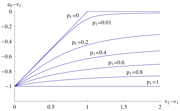
Figure 2: As in Fig. 1: sections of $e_{0}-v_{1}$ as a function of $v_{2}-v_{1}$ for different values of $p_{1}$. For $p_{1}=0$ a quantum phase transition takes place at the critical point $v_{2}-v_{1}=1$.

It is easy to generalize the above result to a case with $m_{\mathscr{V}}>2$. Let us rewrite Eq. (23ba) as

$$-\frac{p_{1}}{e_{0}-v_{1}}+\sum_{k=2}^{m_{\mathscr{V}}}\frac{p_{k}}{(v_{k}-v_{1})-(e_{0}-v_{1})}=1,\qquad e_{0}-v_{1}\leq 0.$$ (23bd)

The unknown $e_{0}-v_{1}$ is a function of the $2(m_{\mathscr{V}}-1)$ parameters $p_{k},v_{k}-v_{1}$, $k=2,\ldots,m_{\mathscr{V}}$. Note that $p_{1}$ is fixed by the normalization condition. We show the graphical construction of the solution of Eq. (23bd) in Fig. 3. For $p_{1}>0$, i.e. $\sum_{k=2}^{m_{\mathscr{V}}}p_{k}<1$, we always have $e_{0}<v_{1}$ and, furthermore, $e_{0}$ is an analytic function of its arguments. When $p_{1}=0$, a singularity of $e_{0}$ shows up, which can be characterized in the following way. Let us define the function

$$W(p_{2},v_{2}-v_{1},\ldots,p_{m_{\mathscr{V}}},v_{m_{\mathscr{V}}}-v_{1})=\sum_{k=2}^{m_{\mathscr{V}}}\frac{p_{k}}{v_{k}-v_{1}}.$$ (23be)

From Eq. (23bd) we see that, if $p_{1}=0$ and $e_{0}<v_{1}$, then

$$W>\sum_{k=2}^{m_{\mathscr{V}}}\frac{p_{k}}{(v_{k}-v_{1})+(v_{1}-e_{0})}=1.$$ (23bf)

On the other hand, if $e_{0}\to v_{1}$ for $p_{1}\to 0$, from the same Eq. (23bd) we have

$$1-W=\lim_{p_{1}\to 0,e_{0}\to v_{1}^{-}}\frac{p_{1}}{v_{1}-e_{0}}\geq 0,$$ (23bg)

i.e. $W\leq 1$. In conclusion, for $p_{1}\to 0$ the below relations hold between $W$ and $e_{0}$

$$W>1\Leftrightarrow e_{0}<v_{1},$$ (23bh)

$$W\leq 1\Leftrightarrow e_{0}=v_{1}.$$ (23bi)

These two equations establish the following scenario for $p_{1}\to 0$. As we move inside the $2(m_{\mathscr{V}}-1)$ dimensional region determined by the condition $W\leq 1$, the rescaled energy $e_{0}$ stalls at its maximum value $e_{0}=v_{1}$. Outside this region, we have $e_{0}<v_{1}$. Therefore, we find that $\nabla e_{0}|_{\mathscr{S}^{+}}\neq 0$ and $\nabla e_{0}|_{\mathscr{S}^{-}}=0$, where $\mathscr{S}^{+}$ and $\mathscr{S}^{-}$ are generic points arbitrary close to the surface $\mathscr{S}$, determined by the condition $W=1$, and such that $W>1$ or $W<1$, respectively. More precisely, we find that on the critical surface $\mathscr{S}$ any directional derivative of $e_{0}$ has a discontinuity for any direction not tangent to $\mathscr{S}$, which, in turn, implies a divergence of any double derivative of $e_{0}$ for any direction not tangent to $\mathscr{S}$.

We observe that according to Eq. (23be) the critical surface is determined by a sum over all the potential levels of the ratios $p_{k}/(v_{k}-v_{1})$. Therefore, even levels very far from the lowest one, $v_{1}$, can contribute to the critical behavior if the corresponding degeneracies are large enough. This is a cooperative phenomenon due to the intrinsic quantum nature of the considered systems.

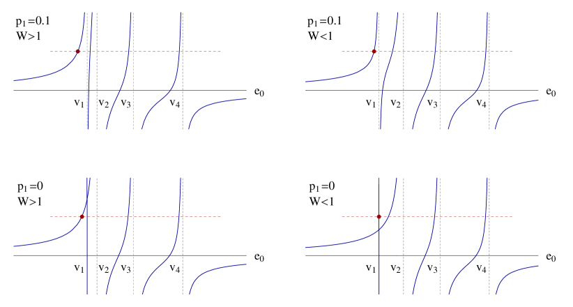
Figure 3: Graphical solution of Eq. (23bd) in a system with four potential levels for $p_{1}=0.1$ (top) and $p_{1}=0$ (bottom) in two cases $W>1$ (left) and $W<1$ (right). The continuous lines are the l.h.s. of Eq. (23bd) plotted as a function of $e_{0}$ whereas the horizontal dashed lines represent the unit level. The rescaled ground-state energy is given by the unique intersection (dots) in the region $e_{0}\leq v_{1}$. For $p_{1}=0$, a singularity shows up at $W=1$, namely $e_{0}$ stalls at its maximum value $e_{0}=v_{1}$ for $W\leq 1$.

We wish to discuss now in more detail the nature of the phase transition corresponding to the above singularity and also determine an order parameter. Let us write the potential operator $\hat{V}$ in terms of the projectors onto the configuration subspaces at fixed potential values

$$\hat{V}=\sum_{V\in\mathscr{V}}V\hat{\pi}_{V},\qquad\hat{\pi}_{V}=\sum_{\bm{n}\in\mathbb{F}:V(\bm{n})=V}|\bm{n}\rangle\langle\bm{n}|.$$ (23bj)

On derivating the ground-state energy $E_{0}$ with respect to a potential level $V$ and using the Hellman-Feynman theorem, we find

$$\frac{\partial E_{0}}{\partial V}=\frac{\partial}{\partial V}\frac{\langle E_{0}|\hat{H}|E_{0}\rangle}{\langle E_{0}|E_{0}\rangle}=\frac{\langle E_{0}|\partial_{V}\hat{H}|E_{0}\rangle}{\langle E_{0}|E_{0}\rangle}=C_{V},$$ (23bk)

where

$$C_{V}=\frac{\langle E_{0}|\hat{\pi}_{V}|E_{0}\rangle}{\langle E_{0}|E_{0}\rangle}=\sum_{\bm{n}\in\mathbb{F}:V(\bm{n})=V}\frac{|\langle\bm{n}|E_{0}\rangle|^{2}}{\langle E_{0}|E_{0}\rangle}$$ (23bl)

is the ground state expectation of the projector $\hat{\pi}_{V}$. On the other hand, in the limit $M\to\infty$ we have $\partial_{V}E_{0}=\partial_{v}e_{0}$ so that by derivating Eq. (23ba) with respect to a generic $v$, we get, in the notation in which the potential levels are ordered,

$$C_{k}=\frac{\partial e_{0}}{\partial v_{k}}=\frac{p_{k}}{(v_{k}-e_{0})^{2}}\left[\sum_{k^{\prime}=1}^{m_{\mathscr{V}}}\frac{p_{k^{\prime}}}{(v_{k^{\prime}}-e_{0})^{2}}\right]^{-1},\quad k=1,\ldots,m_{\mathscr{V}}.$$ (23bm)

Equation (23bm) holds at any point of the $2(m_{\mathscr{V}}-1)$-dimensional space $(p_{2},v_{2}-v_{1},\ldots,p_{m_{\mathscr{V}}},v_{m_{\mathscr{V}}}-v_{1})$. If $p_{1}=0$, from Eqs. (23bh-23bi) and (23bm) we get

$$C_{1}=\cases{1,&$W\leq 1$,\\ 0,&$W>1$,\\ }$$ (23bn)

whereas for $k=2,\ldots,m_{\mathscr{V}}$

$$C_{k}=\cases{0,&$W\leq 1$,\\ \frac{p_{k}}{(v_{k}-e_{0})^{2}}\left[\sum_{k^{\prime}=2}^{m_{\mathscr{V}}}\frac{p_{k^{\prime}}}{(v_{k^{\prime}}-e_{0})^{2}}\right]^{-1},&$W>1$.\\ }$$ (23bo)

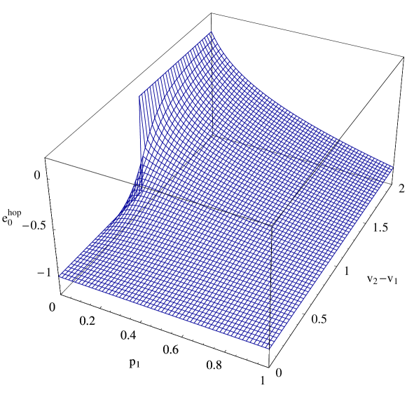
Figure 4: Thermodynamic limit of a system with two potential levels: asymptotic rescaled hopping energy $e_{0}^{\mathrm{hop}}$ as a function of $p_{1}$ and $v_{2}-v_{1}$.

We deduce that in the thermodynamic limit we have the following behavior of the ground state $|E_{0}\rangle$. In the region $W>1$, $|E_{0}\rangle$ turns out to be an analytic function of its arguments $p_{k},v_{k}-v_{1}$, $k=2,\ldots,m_{\mathscr{V}}$, while in the region $W\leq 1$ it collapses into the subspace spanned by the configurations with minimum potential value $V_{1}$. The susceptibilities $\partial_{(v_{k}-v_{1})}C_{k}$ diverge on the critical surface $\mathscr{S}$ determined by the condition $W=1$. Finally, it is simple to check that the asymptotic rescaled hopping energy in the ground state, $e_{0}^{\mathrm{hop}}=\lim_{M\to\infty}\langle E_{0}(M)|\hat{K}|E_{0}(M)\rangle/|E_{0}^{(0)}(M)|$, is given by

$$e_{0}^{\mathrm{hop}}=-\left[\sum_{k=1}^{m_{\mathscr{V}}}\frac{p_{k}}{(v_{k}-e_{0})^{2}}\right]^{-1}.$$ (23bp)

Therefore, the phase for $W\leq 1$ is a frozen phase with $e_{0}^{\mathrm{hop}}=0$, whereas a non vanishing hopping energy is obtained for $W>1$. In Fig. 4 we show the behavior of $e_{0}^{\mathrm{hop}}(p_{1},v_{2}-v_{1})$ in the case with two potential levels described above. For $p_{1}=0$, it is evident the discontinuity of $e_{0}^{\mathrm{hop}}$ at the critical point $W=1$, i.e. $v_{2}-v_{1}=1$.

6 Many-body lattice models: random potential with discrete spectrum

Hereinafter we will focus our analysis on the thermodynamic limit of random potential systems. Equation (23ba) states that for these systems the asymptotic rescaled energy $e_{0}$ is universal, independently of the nature of the hopping operator, provided that $\lim_{M\to\infty}|E_{0}^{(0)}(M)|=\infty$. In this Section we present the results of numerical simulations which help to quantify the rapidity with which this universality is approached by systems with different complexity.

To begin, we investigate quantum particles moving in two-dimensional lattices and interacting via a potential with two random levels. Three cases have been considered: spinless hard-core bosons with long range hopping, spinless hard-core bosons and spinless fermions with first neighbor hopping. The results are displayed in Figs. 5, 6 and 7, respectively. For these systems, in Table 1 we report the noninteracting ground-state energy $E_{0}^{(0)}$ and the average number of active links

$$A_{\mathrm{av}}=\frac{1}{M}\sum_{\bm{n}\in\mathbb{F}}A(\bm{n})$$ (23bq)

as a function of the dimension $M$ of the Fock space. In the case of fermions, due to sign cancellations, the effective average number of active links which is responsible of the potential decorrelation is the difference

$$A_{\mathrm{av}}=\frac{1}{M}\sum_{\bm{n}\in\mathbb{F}}\left(A_{+}(\bm{n})-A_{-}(\bm{n})\right)$$ (23br)

between the active links $A_{\pm}(\bm{n})$ associated with positive or negative jumps, respectively.

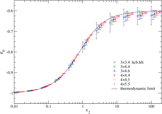
Figure 5: Universality of the thermodynamic limit of random potential systems: rescaled ground-state energy $e_{0}$ as a function of the rescaled potential level $v_{2}$ for systems of spinless hard-core bosons with long range hopping. The random potential has two levels: $V_{1}=0$ with probability $p_{1}=0.6$ and $V_{2}=v_{2}|E_{0}^{(0)}|$ with probability $p_{2}=0.4$. The solid line is the universal thermodynamic limit predicted by Eq. (23ba) whereas the dots corresponds to the numerical results found for the finite-size systems indicated in the legend. Here, $m$$\times$$n.N$ connotes a system of $N$ particles in a $m\times n$ lattice. The error bars represent the standard deviation of the stochastic variable $e_{0}$ as evaluated from an ensemble of 100 exact diagonalizations of the Hamiltonian matrix with the specified random potential.

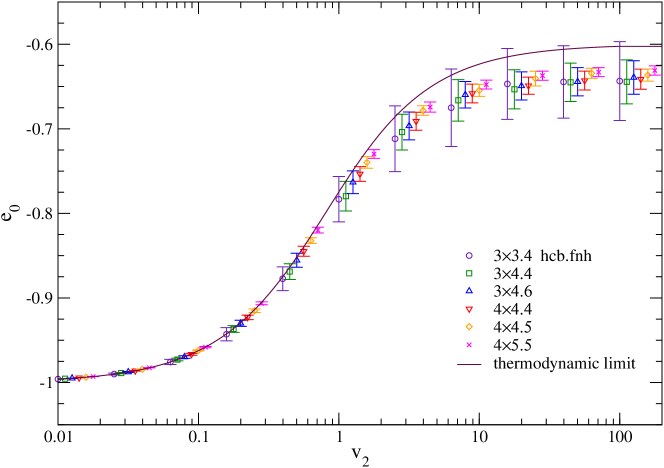
Figure 6: As in Fig. 5 in the case of systems of spinless hard-core bosons with first neighbor hopping.

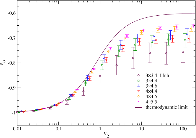
Figure 7: As in Fig. 5 in the case of systems of spinless fermions with first neighbor hopping.

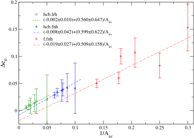
Figure 8: Difference $\Delta e_{0}$ between the rescaled ground-state energy $e_{0}$ predicted in the thermodynamic limit for $v_{2}=100$ by the multinomial formula (23ba) and that obtained in the finite-size systems analyzed in Fig. 5 (hcb.lrh $\circ$), Fig. 6 (hcb.fnh $\triangleleft$) and Fig. 7 (f.fnh $\diamond$) as a function of the inverse of the average number of active links $A_{\mathrm{av}}$. The lines are a weighted linear fit with errors on $\Delta e_{0}$ assumed equal to the standard deviations of $e_{0}$ for the corresponding finite-size systems.

Table 1: For different systems $m$$\times$$n.N$ of $N$ particles in a two-dimensional $m$$\times$$n$ lattice with periodic boundary conditions we report the number of states $M$, the noninteracting ground-state energy $E_{0}^{(0)}$ and the average number of active links $A_{\mathrm{av}}$ in the case of spinless hard-core bosons with long-range (hcb.lrh) and first-neighbor hopping (hcb.fnh) and spinless fermions with first-neighbor hopping (f.fnh).

• 		hcb.lrh		hcb.fnh		f.fnh
  system	000$M$	$E_{0}^{(0)}$	$A_{\mathrm{av}}$	0$E_{0}^{(0)}$	$A_{\mathrm{av}}$	0$E_{0}^{(0)}$	$A_{\mathrm{av}}$
  3$\times$3.4	00126	-20	20	-10.34699	10	0-7	3.33333
  3$\times$4.4	00495	-32	32	-12.10548	11.63636	0-9	4.84848
  3$\times$4.6	00924	-36	36	-13.71426	13.09090	-10	4
  4$\times$4.4	01820	-48	48	-13.25169	12.8	-10	5.52087
  4$\times$4.5	04368	-55	55	-15.30041	14.66666	-12	5.64102
  4$\times$5.5	15504	-75	75	-16.44602	15.78947	-13.23607	7.22394

The case of hard-core bosons with long range hopping presents the closest analogy with a uniformly fully connected model. The number of active links $A(M)$, although being much smaller than the number of states $M$ and diverging more slowly than $M$ for $M\to\infty$, is a constant which does not depend on the configuration $\bm{n}$. In particular, we have that $A(M)=A_{\mathrm{av}}(M)=-E_{0}^{(0)}(M)$ is given by the simple formula $(\textrm{number of sites}-\textrm{number of particles})\times\textrm{number of particles}$. The numerical results, shown in Fig. 5 by dots with error bars, have been obtained by exact diagonalizations of the Hamiltonian matrix for several realizations of the random potential. The error bars represent the standard deviation of the stochastic variable $E_{0}/|E_{0}^{(0)}|$ evaluated in this way. The agreement with the universal curve for $e_{0}$, obtained from Eq. (23ba) as a function of the second rescaled potential level $v_{2}$, worsen by increasing the value of $v_{2}$. However, we have a clear tendency toward the universal result by choosing systems closer and closer to the thermodynamic limit.

For systems with first neighbor hopping, we have a much greater complexity with respect to a uniformly fully connected model. The number of active links is a function of the configuration $\bm{n}$ and, in the case of fermions, a sign problem is also present. Therefore, we expect a convergence to the universal thermodynamic limit slower than that obtained with long range hopping. This is confirmed by the results shown in Figs. 6 and 7. Whereas the trend toward the universal behavior is clear in both cases, for fermions the convergence is indubitably slower than for hard-core bosons.

Note that for practical reasons, essentially the finite amount of memory (4 Gb) of the computer used to perform the numerical diagonalizations, the different systems considered in Figs. 5, 6 and 7 do not have exactly the same density, $\textrm{number of particles}/\textrm{number of lattice sites}$, as it would be convenient in looking at the thermodynamic limit of a lattice particle system. In fact, we have chosen a set of systems in which $M$ and $|E_{0}^{(0)}|$, i.e. $A_{\mathrm{av}}$, possibly both increase compatibly with the condition $M\leq M_{\mathrm{max}}$, where $M_{\mathrm{max}}$ is the size of the largest diagonalizable Hamiltonian matrix. At constant density this set would contain only two or three elements, so we decided to allow for density fluctuations. These fluctuations may reflect a non monotonous approaching to the thermodynamic limit. Such a behavior is quite evident in the fermion case of Fig. 7 where the system 3$\times$4.6 with $M=924$ and $A_{\mathrm{av}}=4$ is closer to the asymptotic universal curve than the next system 4$\times$4.4 which has $M=1820$ and $A_{\mathrm{av}}=5.52087$.

In Fig. 8 we show a quantitative test for the convergence of data in Figs. 5, 6 and 7. The difference $\Delta e_{0}$ between the rescaled ground-state energy of the finite-size systems and the thermodynamic value predicted by the multinomial formula (23ba) is reported, for $v_{2}=100$, as a function of $A_{\mathrm{av}}^{-1}$. In all cases, the data are fitted by straight lines which, compatibly with the associated errors, give $\Delta e_{0}\to 0$ for $A_{\mathrm{av}}^{-1}\to 0$. This behavior corresponds to the scenario depicted in Section 4.3: as the average number of active links $A_{\mathrm{av}}$ diverges, the multinomial formula (23ba) becomes exact with a residual error proportional to $A_{\mathrm{av}}^{-1}$. This law also explains the progressively larger errors observed, at a fixed system size, passing from hard-core bosons with long range hopping to hard-core bosons with first neighbor hopping to fermions with first neighbor hopping, see Eqs. (23bq) and (23br).

The models considered above, even if share some realistic features with systems of interest in physics, have been studied in connection with a toy random potential defined by only two levels $V_{1}$ and $V_{2}$ with assigned probabilities $p_{1}$ and $p_{2}$. For these models, in order to obtain the phase transition in the ground state we must impose the additional condition $p_{1}\to 0$ after the thermodynamic limit has been taken. In the remaining part of this Section, we discuss a more realistic random potential which has the following characteristics: i) the number of levels increases by increasing the number of states $M$, and ii) the probability associated with the lowest level vanishes for $M\to\infty$.

Consider a lattice $\Lambda$ with some ordering of the lattice points $1,2,\dots,n_{|\Lambda|}$ occupied by $N$ quantum particles. As above, we assume that the particles are fermions or hard-core bosons so that the occupation numbers can be $n_{i}=0,1$, $i=1,2,\dots,|\Lambda|$. To each of the $M=|\Lambda|!/(N!(|\Lambda|-N)!)$ Fock states $\bm{n}=(n_{1},n_{2},\dots,n_{|\Lambda|})$ of the system we associate the potential

$$V(\bm{n})=\gamma\sum_{i=1}^{|\Lambda|}n_{i}r_{i}(\bm{n}),$$ (23bs)

where $r_{i}(\bm{n})$ are a set of $|\Lambda|M$ independent random variables assuming the values $0,1$. Let $p$ be the probability that $r_{i}(\bm{n})=1$. Since the Fock states are normalized by the condition $\sum_{i=1}^{|\Lambda|}n_{i}=N$, we have $N+1$ different potential levels $V_{k}=\gamma k$, $k=0,1,\dots,N$ with associated probabilities

$$p_{k} = \frac{N!}{k!(N-k)!}~{}p^{k}(1-p)^{N-k}.$$ (23bt)

Note that $p_{0}$, the probability of the lowest potential level $V_{0}=0$, vanishes for $N\to\infty$ as far as $p>0$.

Before going further, we want to spend a few comments about the introduced potential (23bs). It represents the on site random coupling of a set of $|\Lambda|$ impurities with the particles of the system. The impurities, spins to be concrete, may be in one of two available states with probabilities $p$ and $1-p$. Impurity-impurity interactions are neglected. Moreover, the potential (23bs) treats the impurities itself as classical spins, i.e. it does not take into account the correlations of the state of each single impurity with itself in the presence of different dispositions of the particles in the lattice (Fock states). The latter decoupling could be the effective result of an impurity dynamics fast on the time scale of the evolution of the particle system or of the presence of an external random field.

In the thermodynamic limit $|\Lambda|,N\to\infty$ with $N/|\Lambda|$ constant, the rescaled ground-state energy $e_{0}=E_{0}/|E_{0}^{(0)}|$ is determined by Eq. (23ba). In this limit the sum over the discrete rescaled levels $v_{k}=V_{k}/|E_{0}^{(0)}|$ can be approximated by an integral over $k$ so that Eq. (23ba) reads

$$\int_{0}^{N}\frac{p_{k}}{v_{k}-e_{0}}dk=1,\qquad e_{0}\leq 0.$$ (23bu)

Since Eq. (23bs) is a linear combination of the independent random variables $r_{i}(\bm{n})$, in the thermodynamic limit the distribution of the rescaled potential values, $v_{k}$, becomes infinitely peaked around the mean value $\bar{v}=v_{Np}$,

$$p_{k}\to\delta(k-Np),$$ (23bv)

which inserted into Eq. (23bu) gives

$$\frac{1}{v_{Np}-e_{0}}=1,\qquad e_{0}\leq 0.$$ (23bw)

In conclusion, the solution for the rescaled ground-state energy is

$$e_{0}=\cases{-1+\gamma Np/|E_{0}^{(0)}|,&$\gamma Np/|E_{0}^{(0)}|<1$,\\ 0,&$\gamma Np/|E_{0}^{(0)}|\geq 1$.\\ }$$ (23bx)

Whether or not the solution given above represents a non trivial rescaled ground-state energy depends on how fast the potential levels diverge in the thermodynamic limit with respect to the noninteracting ground-state energy. For a system of fermions with first neighbor hopping $E_{0}^{(0)}$ can be evaluated analytically by Fourier transformation. In one dimension with periodic boundary conditions, at half filling and neglecting spin, for $N\to\infty$ we have $E_{0}^{(0)}\simeq-4\pi^{-1}N\eta$, where $\eta$ is the value of the hopping coefficient between any two first neighbors. Equation (23bx) then becomes

$$e_{0}=\cases{-1+\pi\gamma p/4\eta,&$\pi\gamma p<4\eta$,\\ 0,&$\pi\gamma p\geq 4\eta$.\\ }$$ (23by)

A comparison of $e_{0}$ predicted by the above expression for $p=0.4$ with the values obtained from numerical simulations of finite-size systems is shown in Fig. 9. The main parameters of the simulated systems are given in Table 2. The numerical results are consistent with a phase transition occurring in the thermodynamic limit at $\gamma/\eta=4/\pi p\simeq 3.18$.

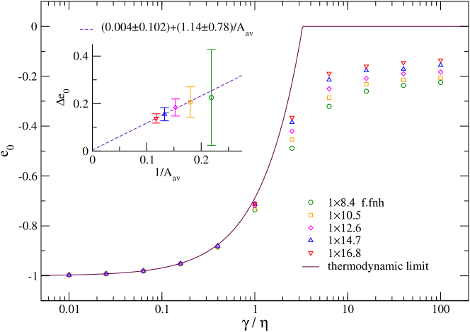
Figure 9: Universality of the thermodynamic limit of random potential systems: rescaled ground-state energy $e_{0}$ as a function of the rescaled potential strength $\gamma/\eta$ for systems, 1$\times$$n.N$, of $N$ spinless fermions with first neighbor hopping in a one-dimensional lattice with $n$ sites. The potential is the impurity potential of Eq. (23bs) with $p=0.4$. The solid line is the universal thermodynamic limit predicted by Eq. (23by) whereas the dots corresponds to the numerical results found for the finite-size systems indicated in the legend. The inset shows a linear fit of $\Delta e_{0}$ vs. $A_{\mathrm{av}}^{-1}$ as displayed in Fig. 8.

Figure 10: As in Fig. 9 in the case of spinless hard-core bosons with long range hopping. The potential is the impurity potential of Eq. (23bs) with $p=0.4$ and $\gamma=\gamma_{1}N$, with $\gamma_{1}$ constant.

Table 2: As in table 1 in the case of one-dimensional systems $1$$\times$$n.N$.

• 		hcb.lrh		hcb.fnh		f.fnh
  system	000$M$	$E_{0}^{(0)}$	$A_{\mathrm{av}}$	0$E_{0}^{(0)}$	$A_{\mathrm{av}}$	0$E_{0}^{(0)}$	$A_{\mathrm{av}}$
  1$\times$8.4	00070	-16	16	0-5.22625	4.57142	0-4.82842	3.42857
  1$\times$10.5	00252	-25	25	0-6.47213	5.55555	0-6.47213	5.55555
  1$\times$12.6	00924	-36	36	0-7.72741	6.54545	0-7.46410	5.45454
  1$\times$14.7	03432	-49	49	0-8.98792	7.53846	0-8.98791	7.53846
  1$\times$16.8	12870	-64	64	-10.25166	8.53333	-10.05467	7.46666

The value of the noninteracting ground-state energy can be given analytically also for spinless hard-core bosons with long range hopping. At half filling with periodic boundary conditions we have $E_{0}^{(0)}=-N^{2}\eta$, where $\eta$ is the value of the hopping coefficient between any two sites. In this case, for $\gamma$ constant the potential levels diverge for $N\to\infty$ slower than $E_{0}^{(0)}$ and Eq. (23bx) always gives $e_{0}=-1$. A non trivial result is obtained assuming $\gamma=\gamma_{1}N$, with $\gamma_{1}$ constant,

$$e_{0}=\cases{-1+\gamma_{1}p/\eta,&$\gamma_{1}p<\eta$,\\ 0,&$\gamma_{1}p\geq\eta$.\\ }$$ (23bz)

In Fig. 10 we show the behavior of Eq. (23bz) for $p=0.4$ in comparison with numerical simulations for finite-size systems. Again, there is a consistent matching with the singularity displayed by $e_{0}$ at $\gamma_{1}/\eta=1/p=2.5$. As discussed in Section 5, in the present case the approach to the thermodynamic behavior is faster (smaller differences $\Delta e_{0}$) with respect to the case of spinless fermions with first neighbor hopping shown in Fig. 9.

Note that, for clarity, we have plotted in Figs. 9 and 10 different curves for $e_{0}$. However, as it is evident by Eqs. (23by) and (23bz), the behavior of the rescaled ground-state energy is universal once it is expressed in terms of the rescaled potential levels $V_{k}/|E_{0}^{(0)}|$, provided, of course, that the same probabilities $p_{k}$ are used.

7 Many-body lattice models: random potential with continuous spectrum

The results obtained in Section 5 are readily extended to the case of a random potential with continuous spectrum. In the thermodynamic limit, for a continuous distribution of rescaled levels $v=\lim_{M\to\infty}V(M)/|E_{0}^{(0)}(M)|$ described by the density $p(v)=\lim_{M\to\infty}p(V(M))$, the equation determining the rescaled energy $e_{0}=\lim_{M\to\infty}E_{0}(M)/|E_{0}^{(0)}(M)|$ reads

$$\int\frac{p(v)}{v-e_{0}}dv=1,\qquad e_{0}\leq v_{\mathrm{min}}.$$ (23ca)

The only point which we have to pay attention to concerns the definition of the lowest potential level. In order to avoid ambiguities, we define $v_{\mathrm{min}}$ as the value of $v$ such that

$$\begin{array}[]{c}p(v_{\mathrm{min}}+\delta)>0\qquad\mbox{and}\qquad p(v_{\mathrm{min}}-\delta)=0,\end{array}$$ (23cb)

with $\delta>0$ arbitrarily small. Note that definition (23cb) does not include the case $v_{\mathrm{min}}=-\infty$, which occurs, for example, if the density $p(v)$ is a Gaussian. However, since for $v_{\mathrm{min}}=-\infty$ we can only have the trivial result $e_{0}=v_{\mathrm{min}}=-\infty$, in the following we will assume $v_{\mathrm{min}}$ finite.

In order to recover the analogous results of Section 5, it is useful to define

$$F(x)=\int\frac{p(v)}{v-x}dv$$ (23cc)

and

$$W=F(v_{\mathrm{min}})=\int\frac{p(v)}{v-v_{\mathrm{min}}}dv.$$ (23cd)

Observe that $F(x)$ is a positive monotonously increasing function for $x\in(-\infty,v_{\mathrm{min}}]$ with

$$-\infty<F(x)\leq W=\sup F\qquad x\in(-\infty,v_{\mathrm{min}}].$$ (23ce)

We have that $e_{0}$ is solution of Eq. (23ca) if $F(e_{0})=1$ and $e_{0}\leq v_{\mathrm{min}}$. If $p(v_{\mathrm{min}})>0$, and therefore $W=\infty$, Eq. (23ce) shows that the solution $e_{0}$ exists, it is unique and smooth, i.e. without singularities with respect to the parameters of the density $p(v)$. If $p(v_{\mathrm{min}})=0$ then, since $\int p(v)dv=1$, we have $W<\infty$. For $1\leq W<\infty$, we still have a unique smooth solution $e_{0}$ of Eq. (23ca), with $e_{0}<v_{\mathrm{min}}$ for $W>1$ and $e_{0}=v_{\mathrm{min}}$ for $W=1$. For $W<1$, Eq. (23ca) has no solution and, as discussed in the discrete case, we have to consider for $e_{0}$ its analytic continuation for $p(v_{\mathrm{min}})\to 0$. More explicitly, we first solve Eq. (23ca) with a modified density $\tilde{p}(v)$ having the same support of $p(v)$ but with $\tilde{p}(v_{\mathrm{min}})>0$ and then evaluate $e_{0}$ as the limit for $\tilde{p}\to p$ of the solution so found. Clearly, this analytic continuation cannot exceed $v_{\mathrm{min}}$ and it is easy to demonstrate that we have $e_{0}=v_{\mathrm{min}}$. In fact, if it were $e_{0}<v_{\mathrm{min}}$, there would be no singularity in the integrand of Eq. (23ca) and the analytic continuation of $e_{0}$ for $\tilde{p}\to p$ would coincide with the solution of Eq. (23ca) with density $p$. As a consequence, we should have $W>F(e_{0})=1$ in contradiction with the hypothesis $W<1$. In conclusion, for $p(v_{\mathrm{min}})=0$ the characterization of the ground state in terms of $W$ is the same as in the discrete case

$$W>1\Leftrightarrow e_{0}<v_{\mathrm{min}},$$ (23cf)

$$W\leq 1\Leftrightarrow e_{0}=v_{\mathrm{min}}.$$ (23cg)

Even when the potential levels $V$ are continuous random variables, the definition (23bj) and the relations (23bk) and (23bl) remain unchanged, and by performing functional derivatives of the rescaled ground-state energy $e_{0}$ with respect to $v$, we have

$$C(v)=\frac{\delta e_{0}}{\delta v}=\frac{p(v)}{(v-e_{0})^{2}}\left[\int\frac{p(v^{\prime})}{(v^{\prime}-e_{0})^{2}}dv^{\prime}\right]^{-1}.$$ (23ch)

Equation (23ch) holds for any density $p(v)$. Again, if $p(v_{\mathrm{min}})=0$, from Eqs. (23cf-23cg) and (23ch) we get

$$C(v_{\mathrm{min}})=\cases{1,&$W\leq 1$,\\ 0,&$W>1$,\\ }$$ (23ci)

whereas for $v>v_{\mathrm{min}}$

$$C(v)=\cases{0,&$W\leq 1$,\\ \frac{p(v)}{(v-e_{0})^{2}}\left[\int\frac{p(v^{\prime})}{(v^{\prime}-e_{0})^{2}}dv^{\prime}\right]^{-1},&$W>1$.\\ }$$ (23cj)

Finally, it is simple to extend Eq. (23bp) for the rescaled hopping energy in the ground state,

$$e_{0}^{\mathrm{hop}}=-\left[\int\frac{p(v)}{(v-e_{0})^{2}}dv\right]^{-1}.$$ (23ck)

Again, if $p(v_{\mathrm{min}})=0$, we see that whereas a non vanishing hopping energy is obtained for $W>1$, the phase for $W\leq 1$ is a frozen phase with $e_{0}^{\mathrm{hop}}=0$.

We conclude this Section by discussing the results of numerical simulations on finite-size systems with a random potential having a continuous spectrum. The systems considered are spinless hard-core bosons with long range hopping in a one-dimensional lattice. Similar results, not shown here, are obtained for spinless hard-core bosons and spinless fermions with first neighbor hopping. The relevant parameters are given in Table 2. No relevant differences are observed in two-dimensional lattices. In Figs. 11 and 12 we illustrate the results for two distinct potentials. In both cases we have $V=\gamma x$ where $x$ is a random variable in the interval $[0,1]$ with normalized constant density $p(x)=1$ in Fig. 11 and with normalized linear density $p(x)=2x$ in Fig. 12. Equation (23ca) predicts, in the thermodynamic limit, a smooth rescaled ground-state energy $e_{0}=E_{0}/|E_{0}^{(0)}|$ for the potential in Fig. 11 and a phase transition for the potential in Fig. 12. In the latter case, the singularity is localized by the condition $W=1$, i.e. at $\gamma/|E_{0}^{(0)}|=2$. The results from the finite-size systems in Figs. 11 and 12 clearly show convergence towards the predicted thermodynamic behavior.

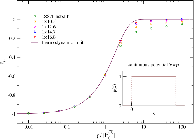
Figure 11: Universality of the thermodynamic limit of random potential systems: rescaled ground-state energy $e_{0}$ as a function of the rescaled potential strength $\gamma/|E_{0}^{(0)}|$ for systems, 1$\times$$n.N$, of $N$ spinless hard-core bosons with long range hopping in a one-dimensional lattice with $n$ sites. The potential randomly associated with the states is $V=\gamma x$, where $x$ is a random variable in the interval $[0,1]$ with normalized constant density $p(x)=1$. The solid line is the universal thermodynamic limit predicted by Eq. (23ca) whereas the dots are the numerical results for the finite-size systems indicated in the legend.

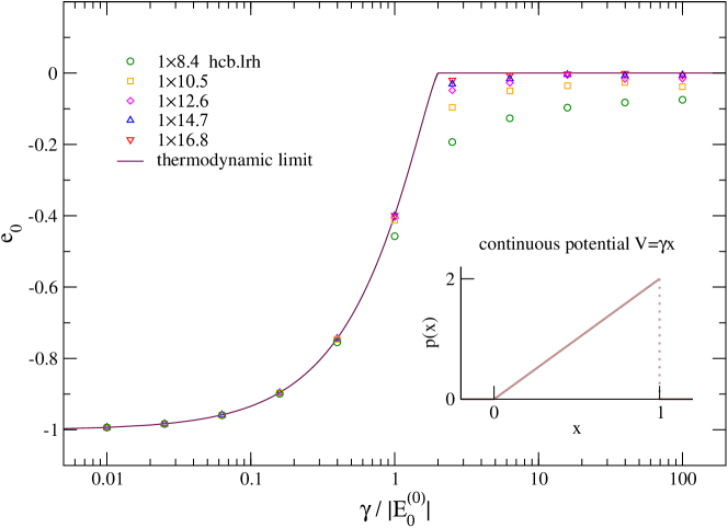
Figure 12: As in Fig. 11 in the case of the potential $V=\gamma x$, where $x$ is a random variable in the interval $[0,1]$ with normalized linear density $p(x)=2x$.

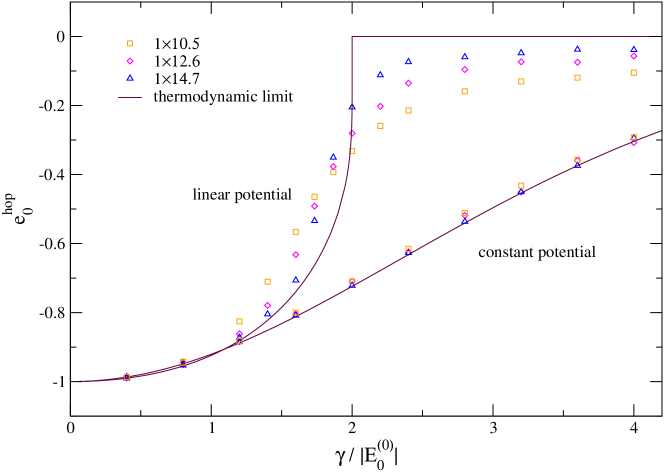
Figure 13: Rescaled hopping energy in the ground state $e_{0}^{\mathrm{hop}}$ as a function of the rescaled potential strength $\gamma/|E_{0}^{(0)}|$ for the systems with constant and linear random potential considered in Figs. 11 and 12. The solid lines are the thermodynamic values predicted by Eq. 23ck whereas the dots are the numerical results for the finite-size systems indicated in the legend.

Finally, in Fig. 13 we show the rescaled hopping energy in the ground state, $e_{0}^{\mathrm{hop}}$, as a function of the rescaled potential strength for the two potentials considered in Figs. 11 and 12. In the case of constant potential, we have a smooth transition between the values $e_{0}^{\mathrm{hop}}=-1$ at $\gamma=0$ and $e_{0}^{\mathrm{hop}}\to 0$ for $\gamma\gg|E_{0}^{(0)}|$. On the other hand, in the case of the linear potential there is a discontinuity in the first derivative of $e_{0}^{\mathrm{hop}}$ as a function of $\gamma$ at $\gamma/|E_{0}^{(0)}|=2$. This behavior is consistent with that observed in the simulations of finite-size systems.

The random potential systems considered in this Section are a many-body generalization of the well-known Anderson models [8], namely a single particle in a $d$-dimensional lattice in the presence of a disorder potential. For the Anderson models with tight binding Hamiltonian the following rigorous results have been established [9]. For $d>1$, the eigenstates of the Hamiltonian undergo a localization phase transition for large disorder; in one dimension, all states are localized for arbitrarily small non zero disorder. It is clear that our analysis does not apply to the single-particle Anderson models, in which the number of active links, i.e. the noninteracting ground-state energy $E_{0}^{(0)}$, remains constant in the limit $M\to\infty$. Note that in the single-particle case the Fock dimension $M$ coincides with the number of lattice points. However, in the many-body case the phase transition predicted by Eq. (23ca) has some analogies with the phase transition in the Anderson models. The transition of the ground state to the frozen phase characterized by $e_{0}^{\mathrm{hop}}=0$ takes place, universally, for $W\leq 1$. In B we show that this condition on the functional $W[p(\cdot)]$ is equivalent to a condition of large disorder, i.e. large support of $p(v)$ or large potential strength. Moreover, as predicted by Eqs. (23ci) and (23cj) and also checked in the numerical simulations for finite-size systems, in the frozen phase the ground state of the system $|E_{0}\rangle$ condensates into a superposition of the Fock states which are eigenstates of the potential operator with eigenvalue $V=V_{\mathrm{min}}$. This condensation, which is a sort of superlocalization in the Fock space, does not correspond, in general, to a localization in the lattice space and takes place for any dimension $d$.

8 Conclusions

We have revisited the probabilistic approach [5, 6, 7] to evaluate the ground state of general matrix Hamiltonian models from a different point of view. The asymptotic probability density of the potential and hopping multiplicities which is the core of the approach is considered known and an exact equation for the ground-state energy $E_{0}$ is obtained in a closed form. For a class of systems, which includes the uniformly fully connected models and the random potential systems, we have that the above mentioned probability density factorizes into separated potential and hopping contributions, the potential part being of multinomial form. This permits to write a very simple scalar equation which relates $E_{0}$ to the lowest eigenvalue of the Hamiltonian operator with zero potential $E_{0}^{(0)}$. Such relation becomes exact in the thermodynamic limit in which $E_{0}^{(0)}$ diverges.

The factorization of the probability density into separated potential and hopping contributions has a different origin in the uniformly fully connected models and in the random potential systems. In the former case, due to the particular structure of the hopping operator which connects with equal probability any state to any other one, the potential values assumed by the system during its evolution are uncorrelated to the number of allowed transitions, equal for any state. In the latter case, the nature of the potential operator ensures that the potential levels are associated randomly with the states of the system. Correlations between potential and hopping values are, however, reintroduced by the dynamics at a degree which depends on the structure of the hopping operator. The correlations disappear if the number of allowed transitions from any state diverges, i.e. $A_{\mathrm{av}}\sim|E_{0}^{(0)}|\to\infty$. This explains why the relation that we have found between $E_{0}$ and $E_{0}^{(0)}$ becomes exact in the thermodynamic limit.

In the thermodynamic limit, we find that the rescaled energy $e_{0}=E_{0}/|E_{0}^{(0)}|$ is a universal function of the potential levels, rescaled by $|E_{0}^{(0)}|$, and of the corresponding degeneracies, for the uniformly fully connected models, or probabilities, for the random potential systems. In the case of the random potential systems this means that $e_{0}$ does not depend on the nature of the hopping operator. In general, if the degeneracy (probability) associated with the lowest potential level vanishes, the ground state of the system undergoes a quantum phase transition between a normal phase and a frozen phase characterized by zero hopping energy. The control parameter $W$ of the phase transition is related to the whole set of levels and corresponding degeneracies (probabilities) of the potential. This parameter measures the inverse amount of the spread (disorder) introduced by the potential operator (random potential). In the frozen phase, corresponding to large spread (disorder), i.e. small $W$, the ground state condensates into the subspace spanned by the states of the system associated with the lowest potential level.

We have performed numerical simulations on different finite-size random potential systems. In particular, we considered many-body lattice systems in which the particles are fermions or hard-core bosons, with long range or first neighbor hopping, in one or two dimensions. The results found for the ground state are nicely consistent with the universal behavior predicted in the thermodynamic limit.

Appendix A Proof of Equation (23af)

Let us rewrite the probability density $\mathcal{P}_{N}(N\bm{\nu})$ in terms of its Fourier transform $\widetilde{\mathcal{P}}_{N}(\bm{q})$

$$P_{N}(N\bm{\nu})=\int d\bm{q}~{}e^{\log[\widetilde{\mathcal{P}}_{N}(\bm{q})]-iN(\bm{q},\bm{\nu})}.$$ (23cl)

If we indicate with $\left\langle\nu_{\alpha_{1}}\ldots\nu_{\alpha_{k}}\right\rangle_{N}^{(c)}$, with $\alpha_{1},\ldots,\alpha_{k}\in\mathscr{H}$, a generic cumulant of order $k$, we have

$$\log{\widetilde{\mathcal{P}}}_{N}(\bm{q})=\log\left\langle e^{iN\left(\bm{\nu},\bm{q}\right)}\right\rangle_{N}=\sum_{k=1}^{\infty}\frac{N^{k}}{k!}\left\langle\left(\bm{\nu},i\bm{q}\right)^{k}\right\rangle_{N}^{(c)}.$$ (23cm)

For any given $N$, due to the inequalities $\left\langle\mu_{\alpha_{1}}\dots\mu_{\alpha_{k}}\right\rangle_{N}\leq N^{k}$, valid for any $k$, and due to the asymmetry $\mathcal{P}_{N}(\bm{\mu})\neq\mathcal{P}_{N}(-\bm{\mu})$, the series in Eq. (23cm) converges for every $\bm{q}\in\mathbb{C}^{m}$ (see, for example [10]).

Let us introduce the rescaled cumulants of order $k$, in a compact notation $\bm{\Sigma}^{(N;k)}$, which are defined as the tensors of rank $k$ with components

$$\Sigma^{(N;k)}_{\alpha_{1},\ldots,\alpha_{k}}=N^{k-1}\left\langle\nu_{\alpha_{1}}\ldots\nu_{\alpha_{k}}\right\rangle_{N}^{(c)},\qquad\alpha_{1},\ldots,\alpha_{k}\in\mathscr{H},$$ (23cn)

and let $\Sigma^{(k)}_{\alpha_{1},\ldots,\alpha_{k}}$ be their asymptotic values

$$\Sigma^{(k)}_{\alpha_{1},\ldots,\alpha_{k}}=\lim_{N\to\infty}N^{k-1}\left\langle\nu_{\alpha_{1}}\ldots\nu_{\alpha_{k}}\right\rangle_{N}^{(c)}=\lim_{N\to\infty}\frac{1}{N}\left\langle N_{\alpha_{1}}\ldots N_{\alpha_{k}}\right\rangle_{N}^{(c)}.$$ (23co)

These limits exist and are finite since the irreducible and finite Markov chain formed by the evolving configurations has a finite correlation length $N_{c}$ with respect to the number of jumps $N$. As a consequence, up to corrections exponentially small in $N/N_{c}$, for $N\to\infty$ we have

$$\log{\widetilde{\mathcal{P}}}_{N}(\bm{q}) =N\sum_{k=1}^{\infty}\frac{i^{k}}{k!}\sum_{\alpha_{1}\in\mathscr{H}}\ldots\sum_{\alpha_{k}\in\mathscr{H}}N^{k-1}\left\langle\nu_{\alpha_{1}}\ldots\nu_{\alpha_{k}}\right\rangle_{N}^{(c)}q_{\alpha_{1}}\ldots q_{\alpha_{k}}$$ (23cp)

$$=Ng(\bm{q}),$$

where the function $g(\bm{q})$ is independent of $N$.

By using the result (23cp) and evaluating the integral in Eq. (23cl) by steepest descent, we find the asymptotic logarithm equality

$$P_{N}(N\bm{\nu})\simeq\exp\left[N\omega(\bm{\nu})\right],$$ (23cq)

where $\omega(\bm{\nu})=g(\bm{q}^{\mathrm{sp}})-i(\bm{q}^{\mathrm{sp}},\bm{\nu})$ is the function at the exponent evaluated in the saddle point $\bm{q}^{\mathrm{sp}}(\bm{\nu})$. Equation (23af) follows immediately.

Appendix B The critical condition $\mathbf{W=1}$ in terms of the disorder

In this Appendix we show that the condition under which the ground state of the system undergoes a quantum phase transition, namely $W=1$, is equivalent to $WA=\mathcal{O}(1)$, where $A$ is the amount of disorder defined as $A=\overline{v}-v_{\mathrm{min}}$.

Let us consider a density $p(v)$ with $p(v_{\mathrm{min}})=0$ and suppose that all the statistical moments of $p(v)$ are finite, $\left\langle v^{k}\right\rangle_{p}<\infty$, with $k$ non negative integer. Let us also suppose, for simplicity, that the density $p(v)$ is symmetric around the mean value $\overline{v}$ so that all the odd centered moments are zero and, furthermore, for any $v$ in the support of $p(v)$ we have

$$|\overline{v}-v|<|\overline{v}-v_{\mathrm{min}}|.$$ (23cr)

By using the geometric series, which is convergent due to the above strict inequality, for any small positive $\delta$ we have

$$\int\frac{p(v)}{v-v_{\mathrm{min}}}dv=\int_{v_{\mathrm{min}}}^{v_{\mathrm{min}}+\delta}\frac{p(v)}{v-v_{\mathrm{min}}}dv+\frac{1}{\overline{v}-v_{\mathrm{min}}}\int_{v_{\mathrm{min}}+\delta}^{v_{\mathrm{max}}}p(v)\sum_{k=0}^{\infty}\frac{\left(v-\overline{v}\right)^{2k}}{\left(\overline{v}-v_{\mathrm{min}}\right)^{2k}}dv.$$ (23cs)

In the interval $[v_{\mathrm{min}}+\delta,v_{\mathrm{max}}]$, for sufficiently small positive $\delta$ we also have

$$\frac{\overline{v}-v}{\overline{v}-v_{\mathrm{min}}}=1-\frac{v-v_{\mathrm{min}}}{\overline{v}-v_{\mathrm{min}}}<1-\frac{\delta}{\overline{v}-v_{\mathrm{min}}}<1.$$ (23ct)

Equation (23ct) implies that the series in the following inequality,

$$\sum_{k=0}^{\infty}\int_{v_{\mathrm{min}}+\delta}^{v_{\mathrm{max}}}p(v)\frac{\left(v-\overline{v}\right)^{2k}}{\left(\overline{v}-v_{\mathrm{min}}\right)^{2k}}dv<\left(v_{\mathrm{max}}-v_{\mathrm{min}}-\delta\right)\sum_{k=0}^{\infty}\left(1-\frac{\delta}{\overline{v}-v_{\mathrm{min}}}\right)^{2k},$$ (23cu)

converges absolutely for any positive (sufficiently small) $\delta$, so that in the second term of the r.h.s. of Eq. (23cs) we can exchange the order in which the operations of integration and series appear. Finally, by performing the limit $\delta\to 0$ and using the fact that $p(v_{\mathrm{min}})=0$, we get

$$W=\frac{1}{\left(\overline{v}-v_{\mathrm{min}}\right)}\sum_{k=0}^{\infty}\frac{\left\langle(v-\overline{v})^{2k}\right\rangle_{p}}{\left(\overline{v}-v_{\mathrm{min}}\right)^{2k}}.$$ (23cv)

From Eq. (23cv) we see that $W$ is a decreasing function of $A=\overline{v}-v_{\mathrm{min}}$ and $W=\mathcal{O}(1)/A$, so that the critical condition amounts to $A=\mathcal{O}(1)$. By recalling that $v=V/|E_{0}^{(0)}|$, in terms of the non rescaled potential the critical condition reads $\overline{V}-V_{\mathrm{min}}=\mathcal{O}(|{E_{0}^{(0)}}|)$. This result is a generalization to many-body systems (in any dimension) of the result established for the single-particle Anderson models with dimension $d>1$ [8, 9].

References

References

- [1] De Angelis G F, Jona-Lasinio G and Sirugue M, 1983 J. Phys. A 16, 2433
- [2] De Angelis G F, Jona-Lasinio G and Sidoravicius V, 1998 J. Phys. A 31, 289
- [3] Beccaria M, Presilla C, De Angelis G F and Jona-Lasinio G, 1999 Europhys. Lett. 48, 243
- [4] Ostilli M and Presilla C, 2004 J. Phys. A 38, 405
- [5] Ostilli M and Presilla C, 2004 New J. Phys. 6, 107
- [6] Presilla C and Ostilli M, 2006 Recent Progress in Many-Body Theories (Series on Advances in Quantum Many-Body Theory vol 9) ed J A Carlson and G Ortiz (Singapore: World Scientific)
- [7] Ostilli M and Presilla C, 2005 J. Stat. Mech. P04007
- [8] Anderson P, 1958 Phys. Rev. 109, 1492
- [9] J. Fröhlich, F. Martinelli, E. Scoppola and T. Spencer, 1985 Commun. Math. Phys. 101, 21
- [10] Shiryayev A N, 1984 Probability (New York: Springer); in particular, see Chapter II, Paragraph 12, Theorem 1