Disentangling single-particle gap by electronic Raman absorption in electron-doped cuprates

Abstract

In the under- to optimal-doping regimes of electron-doped cuprates, it was theoretically suspected that there is a coexistence of superconducting (SC) and antiferromagnetic (AFM) orders. The quasi-particle excitations could be gapped by both orders, and the effective gap is non-monotonic d-wave-like in the momentum space. Alternatively the gap was also speculated as a pure pairing gap. Using an effective microscopic model, we consider the manifestation of the quasi-particle gap in the electronic Raman spectra in a range of doping levels, where the relative strength of the SC and AFM order parameters varies. We demonstrate that from the electronic Raman spectra the effective single-particle gap can be disentangled into contributions from the two distinctive orders. This would help to tell whether the non-monotonic gap is due to the coexistence of SC and AFM orders.

Understanding the pairing symmetry poses a strong constrain on the underlying superconducting mechanism. In hole-doped cuprates a consensus is reached that the predominant pairing channel is $d_{x^{2}-y^{2}}$ hole . The situation is less clear in electron-doped cuprates, such as Nd_2-xCe_xCuO₄ and Pr_2-xCe_xCuO₄. Tunneling tunneling and early Raman measurements Raman s suggest an $s$-wave pairing order parameter, while phase-sensitive measurements consistently imply $d$-wave pairingphase sensitive , the latter of which is also supported by angle-resolved photo-emission spectra (ARPES) ARPES1 and some penetration-depth measurements penetration . It was also speculated that there may be a transition from $d$- to $s$-wave pairing as electron doping level increases ds1 or as temperature decreasesds2 . Even in the $d$-wave picture, the situation is more complicated than that in hole-doped case. The ARPES ARPES2 and the Raman scattering Blumberg experiments on Pr_0.89LaCe_0.11CuO₄ and Nd_1.85Ce_0.15CuO₄, both of which are at the optimal doping, revealed a non-monotonic $d_{x^{2}-y^{2}}$-wave quasi-particle gap, i.e., the maximal gap value occurs between the nodal and antinodal directions instead of at the antinodal direction. On the other hand, a nontrivial evolution of the Fermi surface (FS) was found in electron-doped samples ARPES3 ; ARPES4 . An electron-like FS pockets exist near the ($\pm\pi/4$, $\pm\pi$) and ($\pm\pi$, $\pm\pi/4$) regions in the momentum space for all doping levels in the range $0.10\leq x\leq 0.15$, while a hole-like FS pocket around ($\pm\pi/2$, $\pm\pi/2$) does not emerge untill $x=0.13$. Accordingly, Raman scattering experiments revealed that the relative position of the $B_{1g}$ and $B_{2g}$ peaks changes with doping.Blumberg2 In the optimally doped region, the $B_{2g}$ peak appears at a higher frequency than the $B_{1g}$ one, while in the overdoped region, it appears at a lower frequency than the $B_{1g}$ peak. This was argued as due to the change of the shape of the single-particle gap that originates purely from superconducting pairing Blumberg . This picture is however not sufficient to account for the evolution of the FS ARPES3 ; ARPES4 , and is also in contradiction to the tunnelling measurements that consistently report an $s$-wave feature tunneling . Another difficulty, which is perhaps common in both hole- and electron-doped cuprates, is the large signal in the $A_{1g}$ channel of the Raman spectra a1g , which would have been strongly suppressed by the screening effect in any one-band theory. A phenomenological two-band theory with tunable independent pairing gaps on the two bands seems to account nicely the experimental feature xiangtao . Apart from the $A_{1g}$ puzzle, the microscopic origin of such a theory is yet lacking. Alternatively, the non-monotonic gap was speculated as arising from the coexistence of $d$-wave superconducting (SC) and antiferromagnetic (AFM) orders yuan ; yuan new , even though the SC gap itself is in a typical monotonic $d$-wave form. In the under-doped regime, the hole-pockets do not appear yet, and the single particle excitations would be gapped everywhere in the momentum space. This is then not withstanding the $s$-wave feature in tunnellingtunneling and specific heat measurementsds2 . An issue does arise, however. ARPES and tunnelling only probe single particle excitations, it is not clear how the nontrivial gap manifests in two-particle properties and whether one can disentangle the single particle gap into contributions from different origins. This is the topic of the present paper.

We calculate the electronic Raman spectra in the SC+AFM picture. In a range of doping levels, the relative strength of AFM and SC orders varies, and the Raman spectra reveal distinctive peaks that can be associated to the SC and AFM orders. We also compare the normal state with AFM alone. It turns out that the $B_{2g}$ Raman channel is only sensitive to the SC gap, while the $B_{1g}$ channel responses to both SC and AFM orders. In the presence of a hole-pocket, the $B_{2g}$ channel reveals further a double peak structure, reminiscent of the two sets of normal state FS. Moreover, in all cases that we consider, the SC-related Raman peak in the $B_{2g}$ channel is at lower energy than that in the $B_{1g}$ channel, although the offset becomes much smaller in the coexisting SC+AFM state. As an alternative to elastic neutron scattering measurements (not available yet), these results could help identify the mechanism of the non-monotonic gap and also whether SC+AFM coexists in electron-doped cuprates.

As a handy effective model, we consider the two-dimensional $t$-$t^{\prime}$-$t^{\prime\prime}$-$J$ model hamiltonian,

$$H = -t\sum_{\langle ij\rangle_{1}\sigma}(c^{\dagger}_{i\sigma}c_{j\sigma}+{\rm h.c.})-t^{\prime}\sum_{\langle ij\rangle_{2}\sigma}(c^{\dagger}_{i\sigma}c_{j\sigma}+{\rm h.c.})$$ (1)

$$-t^{\prime\prime}\sum_{\langle ij\rangle_{3}\sigma}(c^{\dagger}_{i\sigma}c_{j\sigma}+{\rm h.c.})+J\sum_{\langle ij\rangle_{1}}\vec{S}_{i}\cdot\vec{S}_{j},$$

where $\langle ij\rangle_{1}$, $\langle ij\rangle_{2}$, $\langle ij\rangle_{3}$ denote the nearest, second-nearest, and third-nearest neighbor bonds. For electron-doped cuprates, this model is defined in the hole picture so that $c_{\sigma}^{\dagger}$ creates a $\sigma$-hole, and no double hole occupancy is implicitly assumed. A hole occupancy of $1-x$ corresponds to a physical electron doping level $x$. Throughout this work, we use the magnitude of the nearest neighbor hopping integral as the unit of energy, so that $t=-1$, $t^{\prime}=0.32$, $t^{\prime\prime}=-0.16$, and $J=0.3$. As usual, the no double occupancy of holes is treated at the slave-boson mean field level where $c_{\sigma}$ is replaced by $\sqrt{x}f_{\sigma}$ in the hopping terms, where $f_{\sigma}$ is the fermionic spinon annihilation operator, and the spin exchange term is decoupled in a standard fashion as $\vec{S}_{i}\cdot\vec{S}_{j}\rightarrow-(3/8)[\chi_{ij}^{*}\sum_{\sigma}f_{i\sigma}^{\dagger}f_{j\sigma}+\Delta_{ij}^{*}(f_{i\downarrow}f_{j\uparrow}-f_{i\uparrow}f_{j\downarrow})+{\rm h.c.}]+(1/2)(m_{j}\sum_{\sigma}\sigma f_{i\sigma}^{\dagger}f_{i\sigma}+i\rightarrow j)+(3/8)(|\chi_{ij}|^{2}+|\Delta_{ij}|^{2})-m_{i}m_{j}$, where consistency requires $\chi_{ij}=\sum_{\sigma}\langle f_{i\sigma}^{\dagger}f_{j\sigma}\rangle$, $\Delta_{ij}=\langle f_{i\downarrow}f_{j\uparrow}-f_{i\uparrow}f_{j\downarrow}\rangle$, and $m_{i}=\sum_{\sigma}\sigma\langle f_{i\sigma}^{\dagger}f_{i\sigma}\rangle/2$. A different setting was used for the decoupling of the spin exchange term in ref.yuan , although one does not expect qualitative changes in the results. Anticipating the uniform AFM order and d-wave SC order, we set $\chi_{ij}=\chi$, $\Delta_{ij}=\pm\Delta$ for $x$- and $y$-bonds respectively, and $m_{i}=\pm m$ for A and B lattice sites respectively. It is convenient to redefine $a_{\sigma}=f_{\sigma}$ on the A-sublattice and $b_{\sigma}=f_{\sigma}$ on the B-sublattice. The mean field Hamiltonian of Eq.(1) can then be written as, in the momentum space,

$$H_{MF} = \sum_{{{\bf k}},\sigma}[\varepsilon_{{\bf k}}(a^{\dagger}_{{{\bf k}}\sigma}b_{{{\bf k}}\sigma}+{\rm h.c.})+(\varepsilon_{{\bf k}}^{\prime}-\mu)(a^{\dagger}_{{{\bf k}}\sigma}a_{{{\bf k}}\sigma}+b^{\dagger}_{{{\bf k}}\sigma}b_{{{\bf k}}\sigma})$$ (2)

$$-2Jm\sigma(a^{\dagger}_{{{\bf k}}\sigma}a_{{{\bf k}}\sigma}-b^{\dagger}_{{{\bf k}}\sigma}b_{{{\bf k}}\sigma})]$$

$$-\sum_{{{\bf k}}}\Delta_{{\bf k}}(a_{{{\bf k}}\uparrow}b_{-{{\bf k}}\downarrow}+b_{{{\bf k}}\uparrow}a_{-{{\bf k}}\downarrow}+{\rm h.c.}),$$

where $\varepsilon_{{\bf k}}=(-2tx-3J\chi/4)(\cos k_{x}+\cos k_{y})$, $\varepsilon_{{\bf k}}^{\prime}=-4t^{\prime}x\cos k_{x}\cos k_{y}-2t^{\prime\prime}x(\cos 2k_{x}+\cos 2k_{y})$, $\Delta_{{\bf k}}=-(3J/4)\Delta(\cos k_{x}-\cos k_{y})$. Here $\mu$ is the chemical potential that fixes the occupancy and the wave vector ${\bf k}$ is restricted in the magnetic Brillouine zone (MBZ). The order parameters are calculated self-consistently at each doping levels. For better convenience, we rewrite the mean field hamiltonian compactly as $H_{MF}=\sum_{{\bf k}}\psi_{{\bf k}}^{\dagger}h_{{\bf k}}\psi_{{\bf k}}$, where $\psi_{{\bf k}}=(a_{{{\bf k}}\uparrow},b_{{{\bf k}}\uparrow},a_{-{{\bf k}}\downarrow}^{\dagger},b_{-{{\bf k}}\downarrow}^{\dagger})^{T}$ are Nambu-Anderson four-spinors, and $h_{{\bf k}}$ is a 4 $\times$ 4 single-particle Hamiltonian,

$$h_{{\bf k}}=\left(\begin{array}[]{c c c c}{A_{1}}&{\varepsilon_{{\bf k}}}&0&{\Delta_{{\bf k}}}\\ {\varepsilon_{{\bf k}}}&{A_{2}}&{\Delta_{{\bf k}}}&0\\ 0&{\Delta_{{\bf k}}}&{A_{3}}&{-\varepsilon_{{\bf k}}}\\ {\Delta_{{\bf k}}}&0&{-\varepsilon_{{\bf k}}}&{A_{4}}\end{array}\right),$$ (7)

where $A_{1}=\varepsilon_{{\bf k}}^{\prime}-\mu-2Jm$, $A_{2}=\varepsilon_{{\bf k}}^{\prime}-\mu+2Jm$, $A_{3}=-\varepsilon_{{\bf k}}^{\prime}+\mu-2Jm$, and $A_{4}=-\varepsilon_{{\bf k}}^{\prime}+\mu+2Jm$. The single particle hamiltonian $h_{k}$ can be easily diagonolized, yielding a set of four eigenvalues $E_{{\bf k},n}$ ($n=1,\cdots,4$) and the corresponding eigenvectors $|{\bf k},n\rangle$ for each ${\bf k}$. The single-particle $4\times 4$ matrix Matsubara greens function $G({\bf k},i{\omega}_{n})=1/(i{\omega}_{n}{\bf 1}-h_{\bf k})$, where ${\bf 1}$ is the $4\times 4$ identity matrix, can be expressed in terms of the eigen states as

$$G({\bf k},i{\omega}_{n})=\sum_{n}\frac{|{\bf k},n\rangle\langle{\bf k},n|}{i{\omega}_{n}-E_{{\bf k},n}},$$ (8)

which forms the basis for further calculations.

The electron Raman scattering measures the spectral function of the fluctuations of the effective charge density $\rho=\sum_{{\bf k}\sigma}\gamma_{\bf k}c_{{\bf k}\sigma}^{\dagger}c_{{\bf k}\sigma}$ where $\gamma_{k}$ is the Raman vertex that describes the second order coupling between electrons and photons literature . In our case the bare Matsubara propagator for $\rho$ can be written as,

$$\chi_{\gamma\gamma}(i\nu_{n})=-\frac{T}{N}\sum_{{{\bf k}},i\omega_{n}}{\rm Tr}[\gamma_{{\bf k}}G({{\bf k}},i\omega_{n})\gamma_{{\bf k}}G({{\bf k}},i\omega_{n}+i\nu_{n})].$$ (9)

Here $T$ is the temperature, $N$ is the number of lattice sites, and

$$\gamma_{\bf k}=({\bf n}_{i}\cdot\nabla_{\bf k})({\bf n}_{s}\cdot\nabla_{\bf k})h_{\bf k}|_{J\rightarrow 0},$$ (10)

is the matrix form of the Raman vertex, where ${\bf n}_{i}$ and ${\bf n}_{s}$ are unit vectors for the polarizations of the incident and scattered lights. Note that the spins do not couple to light to the leading order, so that the spin exchange term does not contribute to the Raman vertex, which is reflected in the formal replacement $J\rightarrow 0$ in the above definition of $\gamma_{\bf k}$. (We do not consider the higher order two-magnon Raman absorptions here.) The summation over $i{\omega}_{n}$ in Eq.(9) can be performed analytically, and we obtain

$$\chi_{\gamma\gamma}(i\nu_{n}) = -\frac{1}{N}\sum_{{\bf k},m,n}[\frac{f(E_{m})-f(E_{n})}{i\nu_{n}+E_{m}-E_{n}}$$ (11)

$$\times{\rm Tr}(\gamma_{\bf k}|{\bf k},m\rangle\langle{\bf k},m|\gamma_{\bf k}|{\bf k},n\rangle\langle{\bf k},n|)],$$

where $f$ is Fermi-Dirac distribution function. The Raman spectral function is then given by

$$R(E)=-\frac{1}{\pi}{\rm Im}\chi(i\nu_{n}\rightarrow E+i0^{+}),$$ (12)

where $E$ is the Raman shift. Note that theoretically $R(E)$ is odd in $E$ and must vanish at $E=0$. For the $B_{1g}$ and $B_{2g}$ channels, the Raman vertices are given by $\gamma_{{\bf k}}^{B_{1g}}=(\gamma_{{\bf k}}^{xx}-\gamma_{{\bf k}}^{yy})/2$ and $\gamma_{{\bf k}}^{B_{2g}}=\gamma_{{\bf k}}^{xy}$, respectively. The $B_{2g}$ channel is $d_{xy}$-symmetric and mainly probes quasi-particle excitations in the nodal directions, while $B_{1g}$ is $d_{x^{2}-y^{2}}$ symmetric and mainly probes excitation in the antinodal directions. These properties enable Raman scattering to selectively probe excitations in the momentum space, and is applied in hole-doped cuprates to verify the d-wave nature of the pairing gap.literature Both $B_{1g}$ and $B_{2g}$ vertices are odd in parity, the Raman absorption in these channels are not re-normalized by Coulomb interactions. In contrast, in the fully symmetric $A_{1g}$ channel, the re-normalization is severe and depends on the detailed band structure (or the Fermi surface harmonics). Due to such complications, we shall concentrate on the simpler $B_{1g}$ and $B_{2g}$ channels in this work.

Before the exposition of Raman spectra in the AFM+SC states, it is instructive to understand, for comparison, the Raman spectra in the non-superconducting states. First, in the normal metallic state with neither AFM nor SC, no Raman spectra are anticipated unless scattering sources are introduced. This is because no finite-energy particle-hole excitations with zero momentum transfer can be achieved in ideal metals. Second, in the normal state with AFM, the band is split into upper and lower bands. Particle-hole excitations vertically across the sub-bands is possible, and one expects nonzero Raman absorption. In this case we show that the Raman response in the $B_{1g}$ channel scales with the square of the AFM order parameter, while the $B_{2g}$ channel is completely insensitive to AFM for the ranges of doping under concern. In the AF state, the Hamiltonian in momentum space can be simplified as $H_{MF}=\sum_{{\bf k}\sigma}\eta_{{\bf k}\sigma}^{\dagger}\xi_{{\bf k},\sigma}\eta_{{\bf k}\sigma}$, where $\eta_{{\bf k}\sigma}=(a_{{{\bf k}}\sigma},b_{{{\bf k}}\sigma})^{T}$, and $\xi_{{\bf k},\sigma}=(\varepsilon_{{\bf k}}^{\prime}-\mu)\sigma_{0}+\varepsilon_{{\bf k}}\sigma_{1}-2Jm\sigma\sigma_{3}$, where $\sigma_{0}$ is the unit $2\times 2$ matrix and $\sigma_{1,3}$ are Pauli matrixes. The spin-dependent single particle Green’s function is given by $g_{\sigma}({\bf k},i{\omega}_{n})=1/(i\omega_{n}\sigma_{0}-\xi_{{\bf k},\sigma})$, which we rewrite for later convenience as,

$$g_{\sigma}({{\bf k}},i\omega_{n}) = \frac{1}{2}\sum_{\nu=\pm 1}\frac{1}{i\omega_{n}+\mu-\varepsilon_{{\bf k}}-\nu E_{k}}$$ (13)

$$\times(\sigma_{0}+\nu\frac{\varepsilon_{{\bf k}}\sigma_{1}-2Jm\sigma\sigma_{3}}{E_{k}}),$$

where $E_{k}=\sqrt{\varepsilon_{{\bf k}}^{2}+4J^{2}m^{2}}$. The Raman vertex is given by $\gamma_{{\bf k}}=(n_{i}\cdot\nabla_{\bf k})(n_{s}\cdot\nabla_{\bf k})\xi_{{\bf k},\sigma})|_{J\rightarrow 0}$. By explicit algebra, we obtain $\gamma_{{\bf k}}^{B_{2g}}=a_{{\bf k}}\sigma_{0}$, where $a_{{\bf k}}=-4t^{\prime}x\sin k_{x}\sin k_{y}$, and $\gamma_{{\bf k}}^{B_{1g}}=b_{{\bf k}}\sigma_{0}+c_{{\bf k}}\sigma_{1}$, where $b_{{\bf k}}=4t^{\prime\prime}x(\cos 2k_{x}-\cos 2k_{y})$ and $c_{{\bf k}}=tx(\cos k_{x}-\cos k_{y})$. In each spin-channel, the Raman response is given by a formula similar to Eq.(9). The total response function summed over spin species is then given by

$$\chi^{B_{2g}} = \frac{1}{4N}\sum_{{\bf k},\sigma,\nu_{1},\nu_{2}}\frac{f(\nu_{2}E_{{\bf k}}+\varepsilon_{{\bf k}}-\mu)-f(\nu_{1}E_{{\bf k}}+\varepsilon_{{\bf k}}-\mu)}{i\nu_{n}+(\nu_{1}-\nu_{2})E_{{\bf k}}}$$ (14)

$$\times{\rm Tr}[a_{{\bf k}}(\sigma_{0}+\nu_{1}\frac{\varepsilon_{{\bf k}}\sigma_{1}-2Jm\sigma\sigma_{3}}{E_{{\bf k}}})$$

$$\times a_{{\bf k}}(\sigma_{0}+\nu_{2}\frac{\varepsilon_{{\bf k}}\sigma_{1}-2Jm\sigma\sigma_{3}}{E_{{\bf k}}}],$$

where $\nu_{1},\nu_{2}=\pm 1$. The trace term gives $2a_{{\bf k}}^{2}(1+\nu_{1}\nu_{2})$, but only the cases with $\nu_{1}=-\nu_{2}$ contributes eventually due to the two fermi functions in the first line. Therefore, $\chi^{B_{2g}}=0$ in the normal state even with AFM order. On the other hand, for the $B_{1g}$ channel, the final result is

$$\chi^{B_{1g}} = \frac{8J^{2}m^{2}}{N}\sum_{{\bf k}}[f(-E_{{\bf k}}+\varepsilon_{{\bf k}}-\mu)-f(E_{{\bf k}}+\varepsilon_{{\bf k}}-\mu)]$$ (15)

$$\times\frac{c_{{\bf k}}^{2}}{E_{{\bf k}}^{2}}(\frac{1}{i\nu_{n}+2E_{{\bf k}}}-\frac{1}{i\nu_{n}-2E_{{\bf k}}}),$$

which scales with $m^{2}$ as we emphasized. We emphasize, however, that the conclusion that $B_{2g}=0$ depends on the bare band structure we use. In principle, including 4-th and further neighbor hopping would cause a nonzero $B_{2g}$, but we expect it to be much weaker as compared to $B_{1g}$ on general grounds.

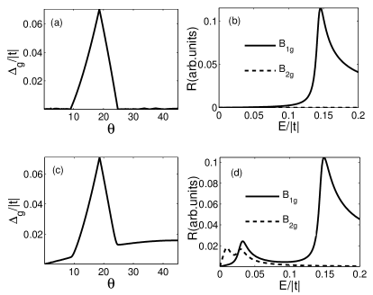
Figure 1: Quasiparticle gap $\Delta_{g}$ and Raman spectra at the doping level $x=0.143$. (a) $\Delta_{g}$ as a function of $\theta$ (in degrees) in the AFM normal state. (b) Raman spectra corresponding to (a). (c) $\Delta_{g}$ as a function of $\theta$ in the AFM+SC state. (d) Raman spectra corresponding to (c).

We now present and discuss the numerical results. The case of $x=0.143$ is presented in Figs.1. In order to understand the Raman spectra we present the quasi-particle gap $\Delta_{g}$ as a function of the angle $\theta$. Henceforth $\theta$ is defined as the angle between ${\bf k}-{\bf Q}$ and $-{\bf Q}$ where ${\bf Q}=(\pi,\pi)$. The gap $\Delta_{g}$ is then defined as the minimum of the quasi-particle energy in the momentum space along a cut of ${\bf k}$ at the same angle $\theta$. Clearly $\Delta_{g}(0)$ measures the gap in the nodal direction, while $\Delta_{g}(45^{\circ})$ measures that in the antinodal region, given the fact that the normal state fermi surface is close to the antinodal point $(\pi,0)$. We begin with the AFM normal state (by simply erasing the SC order from a state with AFM+SC). The gap is presented in Fig.1(a). For $0\leq\theta\leq 10^{\circ}$ and $25^{\circ}<\theta\leq 45^{\circ}$, the normal state gap $\Delta_{g}=0$, roughly reflecting where fermi surfaces appear. For $10^{\circ}<\theta\leq 25^{\circ}$, the normal state is gapped by the AFM order, with a non-monotonic gap $\Delta_{g}$ as a function of $\theta$ due to the underlying band structure. The Raman spectra in this state are presented in Fig.1(b). As we analytically proved, for the model at hand, there is no $B_{2g}$ Raman absorption, but the $B_{1g}$ absorption is strong, and develops a threshold Raman shift roughly twice of the maximal gap in Fig.1(a). Now turning on the SC order, the normal state gap superimposed by the monotonic d-wave pairing gap leads to the gap structure presented in Fig.1(c). Similar result was also reported elsewhere.yuan The maximum of the gap occurs at $\theta=18^{\circ}$. In the experimental caseARPES2 ; Blumberg , $\theta=20^{\circ}$ and $\theta=15^{\circ}$ in $\rm Pr_{0.89}LaCe_{0.11}CuO_{4}$ and $\rm Nd_{1.85}Ce_{0.15}CuO_{4}$, respectively. The corresponding Raman spectra are presented in Fig.1(d). In the $B_{1g}$ channel, the higher energy peak can be associated to the AFM normal state Raman peak but slightly shifted due to pairing. The new lower energy peak is definitely caused by the SC order, as seen from the fact that the energy of this peak is twice of the pairing gap at the anti-nodal direction. The $B_{2g}$ channel, which is silent in the normal state, becomes active in the AFM+SC state, and the peak energy is therefore entirely determined by pairing alone. Interestingly, because of the two kinds of fermi surfaces in the case under concern, two absorption peaks appear in the $B_{2g}$ channel. The energies of the peaks are roughly (but smaller than) twice of the values of the pairing gaps at the two fermi surfaces. This is consistent with the general observation that the $B_{1g}$ Raman vertex is maximal in the the anti-nodal region, whereas $B_{2g}$ vertex is maximal in the nodal region and therefore does not see the full pairing gap. Summarizing, we claim that electronic Raman scattering not only disentangles the different contributions to the total single particle gap, but also tells the number of distinct fermi surfaces, given the monotonic d-wave pairing. Finally, the SC-driven $B_{2g}$ Raman peaks are at smaller energy than the SC-driven $B_{1g}$ peak energy, even though the single particle gap is as non-monotonic as in Fig.1(c). In experimentBlumberg , there appears to be only one peak in both $B_{1g}$ and $B_{2g}$ channel, and the $B_{2g}$ channel is situated at a larger energy. It is also not clear whether an AFM-driven Raman peak is present experimentally.

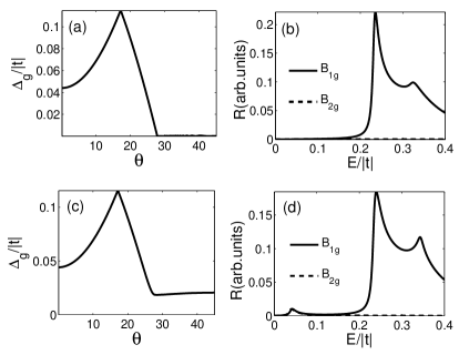
Figure 2: The same plot as Fig.1 but for $x=0.13$.

We now shift to the under-doped AFM+SC regime where AFM is even stronger. For $x=0.13$, the AFM normal state single particle gap is presented in Fig.2(a). Now the gap vanishes only near the anti-nodal region, reflecting the fact that the hole fermi pocket is absent and only one kind of fermi surface appear. The corresponding Raman spectra are presented in Fig.2(b), where again the $B_{2g}$ channel is silent and the $B_{1g}$ channel develops AFM-driven peaks. The additional peak at higher energy arise from the van-Hove singularity in the band structure. Turning on the SC order, the single particle gap is presented in Fig.2(c). Due to the underlying AFM normal state gap, the effective gap here is already nonzero in the nodal direction, and is overall non-monotonic. The corresponding Raman spectra are presented in Fig.2(d). In the $B_{1g}$ channel an SC-driven new Raman peak appears in addition to the AFM-driven peaks at much higher energy. The new peak is at an energy twice of $\Delta_{g}=0.02|t|$ at $\theta=45^{\circ}$. On the other hand, the $B_{2g}$ channel shows a Raman peak with Raman shift very close to but slightly smaller than the energy of the SC-driven peak in the $B_{1g}$ channel. Since the $B_{2g}$ channel is silent in the normal state, we conclude that the gap seen by the $B_{2g}$ channel has nothing to do with the nodal effective gap, but is rather determined by the pairing gap. The single-peak structure seen in the $B_{2g}$ channel is also consistent with the the absence of hole pockets. A disentanglement of single particle gap is therefore again possible.

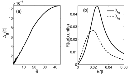
Figure 3: (a) $\Delta_{g}$ as a function of $\theta$ in the SC state at the doping level $x=0.15$. (b) Raman spectra corresponding to (a).

In the over-doped region, for example at $x=0.15$ in our case, the self-consistent calculation yields that AFM order disappears, and we recover a single-band with SC. The situation is then formally similar to the hole-doped case. For completeness we present the quasi-particle excitation gap $\Delta_{g}$ and the corresponding Raman spectra in Fig.4. The gap as a function of $\theta$ is typical of a pure d-wave pairing gap. The $B_{1g}$ channel develops an absorption peak at exactly twice of the maximal pairing gap, while the ratio is roughly $1.5$ in the $B_{2g}$ channel. Because of the absence of AFM order, both channels develop single peaks. The relative peak position is in agreement with experimentBlumberg2 , but the relative intensity of the peaks is not, possibly due to more fine details of the materials. For example, inter-band scattering from the oxygen $p$-band to the upper Hubbard band under concern may modify the effective mass of the electrons, leading to photon-energy dependent changes in the effective Raman vertices. This effect has been experimentally observed.Blumberg

In conclusion, we worked out the consequence of AFM order coexisting with the SC order in the single-particle gap as well as the electronic Raman scattering. In particular we show that using electronic Raman scattering it is possible to disentangle the effective single particle gap into distinctive contributions from AFM and SC orders. Combining the studies in the one-band picture (but with non-monotonic pairing gap) yuan and the phenomenological two-band picture (with independent pairing gaps on the two bands) xiangtao , and by comparing to existing and forthcoming experiments, a strong constrain can be made on the AFM origin of the non-monotonic gap as well as the evolution of the fermi surface with doping in electron-doped cuprates.

- (1) C. C. Tsuei and J. R. Kirtley, Rev. Mod. Phys. 72, 969 (2000).
- (2) Q. Huang, J. F. Zasadzinski, N. Tralshawala, K. E. Gray, D. H. Hinks, J. L. Peng, and R. L. Greene, Nature 347, 369 (1990); Shan L, Y. Huang, H. Gao, Y. Wang, S. L. Li, P. C. Dai, F. Zhou, J. W. Xiong, W. X. Ti, and H. H. Wen, Phys. Rev. B 72, 144506, (2005).
- (3) B. Stadlober, G.Krug, R. Nemetschek, and R. Hackl, Phys. Rev. Lett. 74, 4911, (1995)
- (4) C. C. Tsuei and J. R. Kirtley, Phys. Rev. Lett. 85, 182 (2000); Ariando, D. Darminto, H. -J. H. Smilde, V. Leca, D. H. A. Blank, H. Rogalla, and H. Hilgenkamp, . 94, 167001 (2005).
- (5) N. P. Armitage, D. H. Lu, D. L. Feng, C. Kim, A. Damascelli, K. M. Shen, F. Ronning, and Z.-X. Shen, Phys. Rev. Lett. 86, 1126 (2001); T. Sato, T. Kamiyama, T. Takahashi, K. Kurahashi, and K. Yamada, Science 291, 1517 (2001).
- (6) A. Snezhko, R. Prozorov, D. D. Lawrie, R. W. Giannetta, J. Gauthier, J. Renaud, and P. Fournier, Phys. Rev. Lett. 92, 157005 (2004)
- (7) Amlan Biswas, P. Fournier, M. M. Qazilbash, V. N. Smolyaninova, Hamza Balci, and R. L. Greene, Phys. Rev. Lett. 88, 207004 (2002); John A. Skinta, Mun-Seog Kim, and Thomas R. Lemberger, . 88, 207005 (2002).
- (8) H. Balci and R. L. Greene, Phys. Rev. Lett. 93, 067001 (2004).
- (9) H. Matsui, K. Terashima, T. Sato, T. Takahashi, M. Fujita, and K. Yamada, Phys. Rev. Lett. 95, 017003, (2005).
- (10) G. Blumberg, A. Koitzsch, A. Gozar, B. S. Dennis, C. A. Kendziora, P. Fournier, and R. L. Greene, Phys. Rev. Lett. 88, 107002 (2002).
- (11) N. P. Armitage, F. Ronning, D. H. Lu, C. Kim, A. Damascelli, K. M. Shen, D. L. Feng, H. Eisaki, and Z.-X. Shen, P. K. Mang, N. Kaneko, and M. Greven, Y. Onose, Y. Taguchi, and Y. Tokura, Phys. Rev. Lett. 88, 257001, (2002).
- (12) H. Matsui, K. Terashima, T. Sato, T. Takahashi, S.-C. Wang, H.-B. Yang, H. Ding, T. Uefuji, and K. Yamada, Phys. Rev. Lett. 94, 047005, (2005).
- (13) M. M. Qazilbash, A. Koitzsch, B. S. Dennis, A. Gozar, Hamza Balci, C. A. Kendziora, R. L. Greene, and G. Blumberg, Phys. Rev. B 72, 214510, (2005).
- (14) For hole-doped cuprates, see, , R.Hackl, W. Gläser, P. Müller, D. Einzel, and K. Andres, Phys. Rev. B 38, 7133 (1988); T. Staufer, R. Nemetschek, and R. Hackl, P. Müller, H.Veith, Phys. Rev. Lett. 68, 1069 (1992); R. Nemetschek, O. V. Misochko, B. Stadlober, and R. Hackl, Phys. Rev. B 47, 3450 (1993); for electron-doped ones, see Ref.10 and Ref.13.
- (15) C. S. Liu, H. G. Luo, W. C. Wu, and T. Xiang, Phys. Rev. B 73, 174517 (2006).
- (16) Qingshan Yuan, Feng Yuan, and C. S. Ting, Phys. Rev. B 73, 054501 (2006).
- (17) Qingshan Yuan, Xin-Zhong Yan, and C. S. Ting, cond-matt/0610523.
- (18) See, , T. P. Devereaux, D. Einzel, B. Stadlober, R. Hackl, D. H. Leach, and J. J. Neumeier, Phys. Rev. Lett. 72, 396 (1994); T. P. Devereaux and D. Einzel, Phys. Rev. B 51, 16336 (1995); T. Strohm and M. Cardona, . 55, 12725 (1997); T. Strohm and M. Cardona, Solid State Commun. 104, 233 (1997).