Supplementary Information for cond-mat/0610721: Potok et al. “Observation of the two-channel Kondo effect”

R. M. Potok^1,2,∗, I.G. Rau³, Hadas Shtrikman⁴, Yuval Oreg⁴ and D. Goldhaber-Gordon¹

1 Department of Physics, Stanford University, Stanford, California 94305.

2 Department of Physics, Harvard University, Cambridge, MA, USA.

3 Department of Applied Physics, Stanford University, Stanford, California 94305.

4 Department of Condensed Matter Physics, Weizmann Institute of Science, Rehovot, Israel.

* Present Address: Advanced Micro Devices, Austin, TX.

Measurement techniques

Measurements of differential conductance ($g=dI/dV_{ds}$) were performed in an Oxford TLM dilution refrigerator. (The sample is located inside the mixing chamber.) We measured $g$ using standard ac lockin techniques (using PAR 124a with 116 preamp) at 337 Hz with a RMS excitation ($V_{ex}$) of either 1$\mu V$ or 2$\mu V$, depending on temperature ($eV_{ex}\leq kT$), and measured current with a DL Instruments 1211 preamplifier. To probe nonequilibrium properties, we also added a dc voltage bias $V_{ds}$ to the ac voltage $V_{ex}$ through a passive circuit. Details of the electronics and filtering are contained in Ref. [1].

Determination of $T_{K}$

When the quantum dot has an odd number of electrons and the finite reservoir is not formed (e.g. Fig. 2 in Text), transport through the quantum dot displays the usual signatures of Kondo effect. The Kondo temperature is extracted by fitting the temperature dependence of the conductance (e.g. Fig. 2(b) inset) to Eq. (3) in Text,

$$g(T)=g_{0}f(T/T_{K})+a,$$ (1)

where $f(T/T_{K})$ is the expected empirical form given by  [2]. In Fig. S1(a), $T_{K}$ as a function of $sp$ is given for $c=-282\,mV$ (corresponding to a single Kondo valley in Fig. 2(b) of Text). By measuring the conductance as a function of $sp$ and bias voltage $V_{ds}$ in Fig. S1(b), we observe the Kondo-enhanced density of states at the Fermi level (marked by the arrow). In Fig. S1(c), data similar to those in (a) are shown for a different strength of tunnel coupling to the right lead: $c=-244\,mV$ instead of $-282\,mV$.

We do not have a detailed physical picture of the temperature-independent constant offset $a$ in Eq. (1). When left as a free fitting parameter, we find it does not vary much across a single valley, so we choose to hold it constant as $sp$ is varied over a single valley. At weak coupling to the right lead (coupling gate voltage $c=-282\,$mV), we find that the offset $a=0.21e^{2}/h$ is constant over the Kondo valley near $sp=-230\,$mV. At stronger coupling to the right lead, for the same number of electrons in the small dot ($c=-244\,mV,sp\sim-275\,$mV) we again find a constant offset $a=0.09e^{2}/h$. In Figure 3 of the Text we use the same two values of the offset determined before formation of the finite reservoir, and they work fine for collapsing the data with the finite reservoir formed. Meanwhile, $T_{K}$ varies substantially across a Kondo valley (Fig. S1(a) and (c)), reaching a minimum in mid-valley as expected and as observed in previous experiments [3, 2, 4]. In addition, we note that the main conclusions of the paper are drawn from the scaling curves from Figures 4 and 5 of the Text, which do not depend on the values of $g_{0},a$ and $T_{K}$, but only on the variation in $g$ as a function of bias.

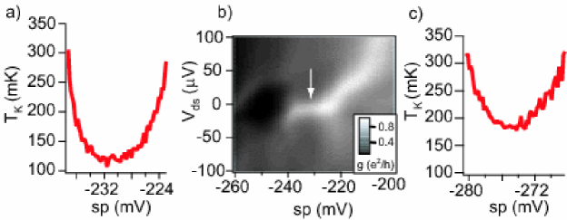
Figure S1: Kondo temperature of the small quantum dot without finite reservoir formed.

Conductance of the double dot system

In Fig. S2(a), conductance as a function of $sp$ and $bp$ is measured through the small dot, along the current path shown in Fig. S2(c). The main, broad conductance features of the small dot depend only on $sp$, as $bp$ is $>1\mu m$ away and thus has a very small capacitance to the small dot. The gate voltage $c$ is set so that the coupling to the finite reservoir is relatively weak. In this regime, the conductance in the Kondo valleys of the small dot, at around $sp$= -260mV and -285mV, is enhanced at low temperature. Gates $sp$ and $bp$ both strongly capacitively couple to the energy of the large dot, affecting its occupancy. The diagonal stripes in the conductance of the small dot are associated with the charge degeneracy points of the large dot. Due to the large capacitive coupling between the two dots, adding an electron to the large dot discretely changes the electrostatic environment of the small dot, which changes its conductance [5]. More complex phenomena, including SU(4) Kondo [6] or two channel Kondo physics [7], may also affect the conductance near the charge degeneracy points. We observe very weak temperature dependence in these regimes – consistent with the exotic Kondo scenarios, but insufficiently distinctive to clarify the relevant physics.

In Fig. S2(b), the same type of data as in (a) is shown for stronger coupling between the two dots, leading to suppressed low-temperature conductance in the Kondo valley at around $sp$ = -280mV. This same effect has also been achieved by decreasing the coupling to either of the two conventional leads, instead of increasing the coupling to the finite reservoir (data not shown.) In Fig. S2(e) conductance as a function of $sp$ and $bp$ is measured through both dots in series, along the current path shown in Fig. S2(d). The charge degeneracy points for both the large and small quantum dots are apparent from these data, revealing the charge stability hexagon (white hexagon superimposed as a guide to the eye).

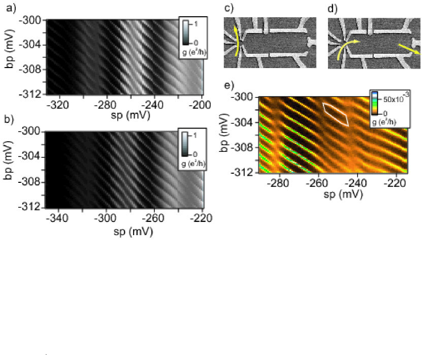
Figure S2: Determining the charge state of the two dots.

Impact of applied magnetic field

As noted in the Text, we applied a magnetic field normal to the plane of the sample in order to deflect electron trajectories so that they cannot travel directly between the entry and the exit point contacts to the small quantum dot. Such direct paths, coexisting with resonant tunneling, give rise to Fano resonances, as seen in previous experiments on quantum dots [8], and in measurements on the present sample at zero magnetic field. Manipulating wavefunctions with modest normal magnetic fields has been used in many other realizations of Kondo effect in quantum dots, for example the achievement of the unitary limit of transport in [4] and tuning of Kondo coupling in a 3-terminal ring [9].

How much impact should this field have on the Kondo physics? Due to the small g factor in GaAs dots, the Zeeman splitting is quite small at the magnetic field we applied (130 mT). Theoretically, magnetic field should be a relevant perturbation to the 2-channel Kondo state (See for example the discussion after Eq. (47) in [10]). However, this should only be the case at very low temperatures $kT<E_{\rm Zeeman}^{2}/kT_{K}$. The field applied in the experiment $B=0.13\;Tesla$ yields a Zeeman energy $E_{\rm Zeeman}=0.13*25=3.25\mu eV$ for GaAs. For $kT_{K}\approx 12\mu{\rm eV}$ in our experiment, the temperature below which the magnetic field should be relevant is $E_{\rm Zeeman}^{2}/kT_{K}\approx.8\mu{\rm eV}\approx 9.5$ mK. This effective energy scale is comparable to the base temperature of the experiments that was around $12mK$, so for 2CK we are never in the regime where magnetic field is a relevant perturbation, with the possible exception of our very lowest temperature. The magnetic field is probably even less important than this calculation suggests, since $E_{\rm Zeeman}$ is often lower by a factor between 1.3 and 3 in a GaAs/AlGaAs heterostructure, where the electron wavefunction leaks into the AlGaAs barrier.

In future, it would be interesting to observe the effect of a larger magnetic field, which should perturb the 2CK state. We would want to apply the field in the plane of the 2DEG, to minimize its effects on orbital states. Applying a field precisely in-plane is non-trivial. We are now setting up to do those measurements.

Note: For 1CK, which is not the main focus of the present work, Zeeman coupling is not a relevant perturbation in the renormalizatin group sense. Provided Zeeman energy is substantially smaller than Kondo temperature (as it is in our experiments) it should have an effect similar to that of bias or temperature $(G=G_{0}-{\rm const}_{1}\cdot(T/T_{K})^{2})-{\rm const}_{2}\cdot(eV_{\rm ds}/kT_{K})^{2})-{\rm const}_{3}\cdot(g\mu_{B}B/kT_{K})^{2})$, where the three constants are all of order unity. In our experiments, $g\mu_{B}B$ is roughly one to three times $kT_{\rm base}$, depending on the exact g-factor. Since all the perturbations are substantially smaller than the Kondo temperature, the presence of the magnetic field should not substantially affect the scaling of conductance with temperature and bias.

Scaling analysis of 1CK data

In the main Text we demonstrated that the data we identify as reflecting a symmetric 2CK state cannot be described by a Fermi liquid scaling appropriate to 1CK. It is important to establish the converse: that the data we identify as reflecting 1CK do not follow 2CK scaling. We show this in Fig. S3, where the 1CK data presented in Figure 4 of the Text are seen to scale as expected for 1CK and not as expected for 2CK. From Eq. (4) of the Text, the expected scaling for 1CK is

$$\frac{g(0,T)-g(V_{ds},T)}{T^{\alpha}}=\kappa\left(\frac{eV_{ds}}{kT}\right)^{2},$$ (2)

with $\alpha=2$ and $\kappa=0.82\frac{g_{0}}{T_{K}^{2}}$ [11]. In Fig. S3(a), we show the same 1CK scaling plot as in Fig. 4(d) of the Text, but without normalizing to account for $T_{K}$ or $g_{0}$.

In Fig. S3(b), we scale the same data from Fig. S3(a) as would be appropriate for 2CK behavior, i.e. with $\alpha=0.5$. In Fig. S3(c) and (d) we simulate idealized 1CK (Fermi liquid) data and scale them as would be appropriate for 1CK ($\alpha=2$, (c)) and 2CK ($\alpha=0.5$, (d). Comparing Fig. S3(b) and (d), the simulated 1CK data deviate from perfect 2CK scaling very similarly to how the actual 1CK data deviate. Note that the qualitative behavior is the opposite of what one would expect from a breakdown of scaling when approaching some finite energy scale (e.g. $T_{K}$): curves at higher temperatures fall inside those at lower temperatures, instead of “peeling off” toward the outside above a certain bias voltage. The nonlinear fits presented in the Text quantify these observations: the best fit for $\alpha$ is $1.72\pm 0.4$ for the 1CK data and $0.62\pm 0.21$ for the symmetric 2CK data, clearly distinguishable from each other, and both consistent with theoretical expectations ($\alpha=2$ and $0.5$, respectively.)

Figure S3: Scaling of 1CK

Comparison of theory and experiment for $\kappa$, 1CK scaling prefactor

As noted in the Text, the value of $\kappa$ depends on the underlying model (Kondo effect can be derived from various different models), numerical calculations ($\kappa$ connects low-energy behavior to high-energy behavior, and no analytical results can make this link quantitatively), and proximity to the symmetric 2CK point (near the symmetric point, $T_{\rm K}$ is replaced by $T_{\Delta}$, a measure of the asymmetry). Here we outline how to determine $\kappa$ theoretically, and we comment on the link to our experimental result.

First, a Kondo energy scale (or Kondo temperature) is only a crossover scale, so different definitions could yield values differing by some constant multiple. We want results that are independent of these initial definitions. Theoretically, the Kondo temperature is usually defined in terms of a thermodynamic quantity such as susceptibility rather than a dynamic quantity such as electrical conductance, so we must use a model to link the two. According to Costi [12],

$$g(T)=g_{0}\left(1-\frac{\pi^{4}}{16}\left(\frac{T}{T_{0}}\right)^{2}\right),$$

[13]

where $T_{0}$ is defined according to

$$\chi(T=0)=\frac{(g\mu)^{2}}{4kT_{0}}.$$

Now

$$\kappa=g_{0}\left(\frac{\pi^{2}}{4T_{0}}\right)^{\alpha}\frac{3}{2\pi^{2}}$$

For the case $\alpha=2$ we find

$$\kappa=g_{0}\frac{3\pi^{4}}{32\pi^{2}T_{0}^{2}}=\frac{3\pi^{2}}{32}\frac{1}{T_{0}^{2}}.$$

Next, we must link the thermodynamically-defined Kondo scale $T_{0}$ to $T_{\rm K}$, defined according to $g(T_{\rm K})=g_{0}/2$ [13]. Costi’s NRG calculations suggest that this link depends mildly on details of the system such as the dimensionality of the leads. For 2D leads, $T_{\rm K}=0.94T_{0}$. This yields $\kappa=0.82\frac{g_{0}}{T_{K}^{2}},$ as reported in the Text. This is in rough but satisfactory agreement with our experimentally-extracted value $\kappa=0.25$ for both 1CK with the conventional leads and 1CK with the finite reservoir. Note that other approaches to the basic Kondo model may or may not give the same result. A. Schiller’s calculations based on an exactly-solvable model at the Toulouse limit give

$$g(T)=g_{0}\left(1-\frac{\pi^{4}}{48}\left(\frac{T}{T_{0}}\right)^{2}\right),$$

yielding a value of $\kappa$ three times smaller than that of the other models, and in almost perfect agreement with our experimental results. Apart from this (perhaps serendipitous) match we have no reason to believe that the exactly-solvable model at the Toulouse limit is a better description of the low-energy properties of our system than Nozières’s Fermi liquid approach.

A final complication in quantitative comparison of theory and experiment is that our measurements are not very far from the symmetric 2CK, so $T_{\rm K}$ should be replaced by $T_{\Delta}$. It’s not clear whether $T_{\Delta}$ should act the same as $T_{\rm K}$ at both low and high energies. Therefore, it will be interesting to perform these same analyses on a two-lead dot which exhibits simple 1CK behavior, with no link to 2CK.

Raw data for 2CK scaling analysis

Fig. S4 shows the raw data used in the 2CK scaling analysis. These data were obtained under conditions similar to those for the $c=-260\,$mV curve in Fig. 5(e) in the Text, which shows differential conductance at widely-spaced values of the coupling gate voltage $c$. Since the parameters of the system had shifted since acquisition of the data in Fig. 5(e), the coupling gate had to be changed to $c=-258\,$mV. For the scaling analysis (Fig. 5(f) of Text), to reduce the noise in the value of $g(V_{\rm ds}=0)$ we averaged the conductances at $-1\mu$V, $0$, and $1\mu$V.

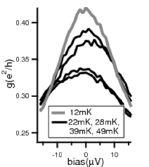
Figure S4: Unscaled conductance curves at different temperatures at the 2CK point.

Match of raw data to 2CK predictions

Fig. S5 shows the 12 mK raw data used in the 2CK scaling analysis (gray curve from Fig. S4.) A parabolic fit works only at low bias. In contrast, a square-root fit ($g(V_{\rm ds})=g_{0}-g_{1}\sqrt{V_{\rm ds}}$, with $g_{0}$ and $g_{1}$ as fit parameters, Fig. S6) works well at intermediate bias ($V_{\rm ds}=5$ to $15\mu$V) This crossover from quadratic to square-root behavior at bias a few times $kT$ agrees with conformal field theory predictions for 2CK [14, 10, 15]. This match is reinforced by the more complete scaling analysis in Fig. 5(f).

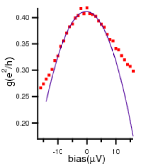
Figure S5: Parabolic fit to $g(V_{\rm ds})$ at small bias.

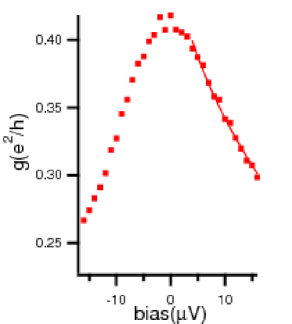
Figure S6: Square-root fit to $g(V_{\rm ds})$ at intermediate bias.

Asymmetry of coupling to the two conventional leads that comprise the “infinite reservoir”

The tunnel barriers between the local site and the two conventional leads were intentionally tuned to be asymmetric, for two reasons:

a. Existing theoretical calculations for 2CK (and 1CK) give density of states in equilibrium. Our scaling measurements involve applying finite bias from one lead to the other. The strong asymmetry between the couplings to the two leads means that the local site remains essentially in equilibrium with the more strongly-coupled lead, validating quantitative comparison with predictions.

b. The symmetric 2CK state occurs when $J_{1}=J_{2}$, which requires that $\Gamma_{\rm fr}\approx\Gamma_{\rm ir}$, where $\Gamma_{\rm ir}$ is the sum of the tunnel rates to the two conventional leads. If all three tunnel barriers were equal, we would instead have $\Gamma_{\rm fr}=0.5\Gamma_{\rm ir}$. It turns out to be easiest to tune the system by first matching the tunnel barrier of the finite reservoir to that of one of the open leads. With the finite reservoir open to the outside world (gate $n$ grounded) and one conventional lead fully pinched off, we maximized the two-terminal conductance between the other conventional lead and the infinite reservoir (in fact we found it could be very near $2e^{2}/h$, usually $\sim 1.8e^{2}/h$). This means $\Gamma_{\rm fr}\approx\Gamma_{\rm ir}$. We then slowly cracked open the second conventional lead and closed off the finite reservoir from the outside world (using gate $n$). In this way, we maintained $\Gamma_{\rm fr}$ near $\Gamma_{\rm ir}$, as needed for $J_{1}=J_{2}$. We felt this was the best method to ensure nearly equal $\Gamma$s and $J$s.

Bibliography

- S1. R. M. Potok. Ph.D. dissertation. Harvard University, 2006.
- S2. D. Goldhaber-Gordon, Jörn Göres, Hadas Shtrikman, D. Mahalu, U. Meirav, and M. A. Kastner. From the Kondo regime to the mixed-valence regime in a single-electron transistor. Physical Review Letters, 81:5225, 1998.
- S3. F. D. M. Haldane. Scaling theory of the asymmetric Anderson model. Physical Review Letters, 40:416–419, 1978.
- S4. W. G. van der Wiel, S. De Franceschi, T. Fujisawa, J. M. Elzerman, S. Tarucha, and L. P. Kouwenhoven. The Kondo effect in the unitary limit. Science, 289:2105 – 8, 2000.
- S5. A. C. Johnson, C. M. Marcus, M. P. Hanson, and A. C. Gossard. Coulomb-modified Fano resonance in a one-lead quantum dot. Physical Review Letters, 93:106803 – 4, 2004.
- S6. K. Le Hur, P. Simon, and L. Borda. Maximized orbital and spin Kondo effects in a single-electron transistor. Physical Review B, 69:45326, 2004.
- S7. E. Lebanon, A. Schiller, and F. B. Anders. Enhancement of the two-channel Kondo effect in single-electron boxes. Physical Review B, 68:155301, 2003.
- S8. J. Göres, D. Goldhaber-Gordon, S. Heemeyer, M.A. Kastner, Hadas Shtrikman, D. Mahalu, and U. Meirav. Fano resonances in electronic transport through a single-electron transistor. Physical Review B, 62:2188–94, 2000.
- S9. R. Leturcq, L. Schmid, K. Ensslin, Y. Meir, D. C. Driscoll, and A. C. Gossard. Probing the Kondo density of states in a three-terminal quantum ring. Physical Review Letters, 95:126603, 2005.
- S10. M. Pustilnik, L. Borda, L.I. Glazman, and J. von Delft. Quantum phase transition in a two-channel-Kondo quantum dot device. Physical Review B, 69:115316, 2004.
- S11. This equation describes the low-energy Fermi-liquid behavior, at an energy scale substantially below [16]. for a channel-asymmetric 2CK system, the crossover scale is replaced by , where is a measure of the channel asymmetry which goes to zero when [10].
- S12. T. Costi, private communication. we have confirmed that this link between conductance and susceptibility, both at low energies, agrees exactly with results of I. Affleck, of P. Nozières, and of M. Pustilnik and L.I. Glazman.
- S13. Because we have a temperature-independent conductance offset, we replace with in this formula, for comparison with the data on 1CK with the conventional leads (fig. 4(d) of text) – the analysis is similar for 1CK with the finite reservoir, but the temperature-dependence has the opposite slope.
- S14. I. Affleck and A. W. W. Ludwig. Exact conformal-field-theory results on the multichannel Kondo effect: single-fermion Green’s function, self-energy, and resistivity. Physical Review B, 48:7297 – 321, 1993.
- S15. J. von Delft, A. W. W. Ludwig, and V. Ambegaokar. The 2-channel Kondo model. II. CFT calculation of non-equilibrium conductance through a nanoconstriction containing 2-channel Kondo impurities. Annals of Physics, 273:175 – 241, 1999.
- S16. K. Majumdar, A. Schiller, and S. Hershfield. Nonequilibrium Kondo impurity: Perturbation about an exactly solvable point. Physical Review B, 57:2991 – 2999, 1998.