Basis of a non Riemannian Geometry within the Equilibrium Thermodynamics

Abstract

Microcanonical description is characterized by the presence of an internal symmetry closely related with the dynamical origin of this ensemble: the reparametrization invariance. Such symmetry possibilities the development of a non Riemannian geometric formulation within the microcanonical description of an isolated system, which leads to an unexpected generalization of the Gibbs canonical ensemble and the classical fluctuation theory for the open systems, the improvement of Monte Carlo simulations based on the canonical ensemble, as well as a reconsideration of any classification scheme of the phase transitions based on the concavity of the microcanonical entropy.

I Introduction

Generally speaking, a phase transition brings about a sudden change of the macroscopic properties of a system while smoothly varying of a control parameter. The mathematical description of phase transitions in the conventional Thermodynamics is based on the loss of analyticity (the appearance of a singularity in the firsts derivatives) of the (gran)canonical thermodynamic potential gallavotti ; Gold , which are related with the existence of zeros in the partition function appearing with the imposition of the thermodynamic limit yang-lee .

However, phase transitions are also relevant in systems outside the thermodynamic limit. A nontrivial example is the nuclear multifragmentation, a phenomenon taking place as a consequence of peripheral collisions of heavy ions, which can be classified under the light of the new developments as a first-order phase transition moretto ; Dagostino .

The key for taking into account the phase transitions in isolated systems outside the thermodynamic limit is the consideration of the well-known Boltzmann Principle:

$$S_{B}=\ln W$$

             (1)

his celebrated gravestone epitaph. Since $W$ is the number of microscopic states compatible with a given macroscopic state, the Boltzmann entropy 1 is a measure of the size of the microcanonical ensemble. Within Classical Statistical Mechanics $W$ is just the microcanonical accessible phase space volume, that is, a geometric quantity. This explains why the entropy 1 does not satisfy the concavity and the extensivity properties, neither demands the imposition of the thermodynamic limit or a probabilistic interpretation like the Shannon-Boltzmann Gibbs extensive entropy:

$$S_{e}=-\sum_{k}p_{k}\ln p_{k}.$$ (2)

As already shown by Gross gro1 ; gro na , phase transitions in small systems could be classified within the microcanonical ensemble throughout the ”topology” of the Hessian of the Boltzmann entropy.

We will show in the present work that the microcanonical description is characterized by the existence of an internal symmetry: the reparametrization invariance. We shall demonstrate that the presence of this symmetry implies a revision of classification of phase transitions based on the concavity of the entropy and the theory of the statistical ensembles derived from microcanonical basis.

II Reparametrization invariance

II.1 Geometrical basis

Universality of the microscopic mechanisms of chaoticity provides a general background for justifying the necessary ergodicity which supports a thermostatistical description with microcanonical basis for all those nonintegrable many-body Hamiltonian systems PF1 ; PF2 ; lieberman ; pettini 51 ; cohenG . Thus, the microcanonical ensemble:

$$\hat{\omega}_{M}\left(I,N\right)=\frac{1}{\Omega\left(I,N\right)}\delta\left\langle I-\hat{I}\left(X\right)\right\rangle,$$ (3)

is just a dynamical ensemble where every macroscopic characterization has a direct mechanical interpretation. Here, $X$ represents a given point of the phase space $\Gamma$ and $\hat{I}\left(X\right)=\left\{\hat{I}^{1}\left(X\right),\hat{I}^{2}\left(X\right),\ldots\hat{I}^{n}\left(X\right)\right\}$ are all those relevant (analytical) integrals of motion determining the microcanonical description in a given application (since Poincare-Fermi theorem PF1 ; PF2 : the total energy, the angular and linear momentum).

The admissible values of the set of integrals of motion $\hat{I}\left(X\right)$ could be considered as the ”coordinate points” $I=\left\{I^{1},I^{2},\ldots I^{n}\right\}$ of certain subset $\mathcal{R}_{I}$ of the n-dimensional Euclidean space $\mathcal{R}^{n}$. Each of these points determines certain sub-manifold $\mathcal{S}_{p}$ of the phase space $\Gamma$ :

$$X\in\mathcal{S}_{p}\equiv\left\{X\in\Gamma\left|\forall k~{}I^{k}\left(X\right)=I^{k}\right.\right\},$$ (4)

in which the system trajectories spread uniformly in accordance with the ergodic character of the microscopic dynamics. Such sub-manifolds defines a partition $\Im$ of the phase space $\Gamma$ in disjoint sub-manifolds:

$$\Im=\left\{\mathcal{S}_{p}\subset\Gamma\left|~{}{\displaystyle\bigcup_{p}}\mathcal{S}_{p}=\Gamma~{};~{}\mathcal{S}_{p}\cap\mathcal{S}_{q}=\varnothing\right.\right\}.$$ (5)

Definitions 4 and 5 allow the existence of a bijective map $\psi_{I}$ between the elements of $\Im$ (sub-manifolds $\mathcal{S}_{p}\subset\Gamma$) and the elements of $\mathcal{R}_{I}$ (points $I\in\mathcal{R}^{n}$):

$$\psi_{I}:\Im\rightarrow\mathcal{R}_{I}\equiv\left\{\forall\mathcal{S}_{p}\in\Im\left(\Gamma\right)~{}\exists I\in\mathcal{R}_{I}\subset\mathcal{R}^{n}\right\}.$$ (6)

Thus, the partition $\Im$ has the same topological features of the n-dimensional Euclidean subset $\mathcal{R}_{I}$. For this reason $\Im$ will be referred as the abstract space of the integrals of motions. We say that the map $\psi_{I}$ defines the n-dimensional Euclidean coordinate representation $\mathcal{R}_{I}$ of the abstract space $\Im$.

Let us now to consider another subset $\mathcal{R}_{\varphi}\subset\mathcal{R}^{n}$ with the same diffeomorphic structure of the subset $\mathcal{R}_{I}$ and the following diffeormorphic map $\varphi$ among them:

$$\varphi:\mathcal{R}_{I}\rightarrow\mathcal{R}_{\varphi}\equiv\left\{\forall I\in\mathcal{R}_{I}~{}\exists\varphi\in\mathcal{R}_{\varphi}\left|\det\left(\frac{\partial\varphi^{j}}{\partial I^{k}}\right)\not=0\right.\right\}.$$ (7)

We say that the map $\varphi$ represents a general reparametrization change of the microcanonical description since it allows us to introduce another n-dimensional Euclidean coordinate representation $\mathcal{R}_{\varphi}$ by considering the bijective map $\psi_{\varphi}=\psi_{I}o\varphi^{-1}$:

$$\psi_{\varphi}:\Im\rightarrow\mathcal{R}_{\varphi}\equiv\left\{\forall\mathcal{S}_{p}\in\Im~{}\exists\varphi\in\mathcal{R}_{\varphi}\subset\mathcal{R}^{n}\right\}.$$ (8)

The above reparametrization change $\varphi$ also induces the following reparametrization of the relevant integrals of motion $\varphi_{X}:\hat{I}\left(X\right)\rightarrow\hat{\varphi}\left(X\right)$, where:

$$\hat{\varphi}\left(X\right)=\left\{\varphi^{1}\left\langle\hat{I}\left(X\right)\right\rangle,\varphi^{2}\left\langle\hat{I}\left(X\right)\right\rangle,\ldots\varphi^{n}\left\langle\hat{I}\left(X\right)\right\rangle\right\}.$$ (9)

Since $\hat{I}\left(X\right)$ are integrals of motions, every $\varphi^{k}\left\langle\hat{I}\left(X\right)\right\rangle\in\hat{\varphi}\left(X\right)$ will be also an integral of motion. The bijective character of the reparametrization change $\varphi:\mathcal{R}_{I}\rightarrow\mathcal{R}_{\varphi}$ allows us to say that the sets $\hat{\varphi}\left(X\right)$ and $\hat{I}\left(X\right)$ are equivalent representations of the relevant integrals of motion of the microcanonical description because of they generate the same phase space partition $\Im$.

The interesting question is that the microcanonical ensemble is invariant under every reparametrization change. Considering the identity:

$$\delta\left\langle\varphi-\hat{\varphi}\left(X\right)\right\rangle\equiv\left|\frac{\partial\varphi}{\partial I}\right|^{-1}\delta\left\langle I-\hat{I}\left(X\right)\right\rangle,$$ (10)

where $\left|\partial\varphi/\partial I\right|\not=0$ is the Jacobian of the reparametrization change $\varphi$, the phase space integration leads to the following transformation rule for the microcanonical partition function:

$$\Omega\left(\varphi,N\right)=\left|\frac{\partial\varphi}{\partial I}\right|^{-1}\Omega\left(I,N\right),$$ (11)

leading in this way to the reparametrization invariance of the microcanonical distribution function:

$$\frac{1}{\Omega\left(\varphi,N\right)}\delta\left\langle\varphi-\hat{\varphi}\left(X\right)\right\rangle\equiv\frac{1}{\Omega\left(I,N\right)}\delta\left\langle I-\hat{I}\left(X\right)\right\rangle.$$ (12)

A corollary of the identity 12 is that the Physics derived from the microcanonical description is reparametrization invariant since the expectation values $\left\langle O\right\rangle$ of any macroscopic observable $\hat{O}\left(X\right)$ obtained from the microcanonical distribution function $\hat{\omega}_{M}\left(X\right)$ exhibits this kind of symmetry:

$$\left\langle O\right\rangle=\int\hat{O}\left(X\right)\hat{\omega}_{M}\left(X\right)dX\Rightarrow\left\langle O\right\rangle\left(\varphi,N\right)=\left\langle O\right\rangle\left(I,N\right).$$ (13)

The reparametrization invariance does not introduce anything new in the macroscopic description of a given system, except the possibility of describing the microcanonical macroscopic state by using any coordinate representation of the abstract space $\Im$, a situation analogue to the possibility of describing the physical space $\mathcal{R}^{3}$ by using a Cartesian coordinates $\left(x,y,z\right)$ or a spherical coordinates $\left(r,\theta,\varphi\right)$. Thus, we can develop a geometrical formulation of Thermostatistics within the microcanonical ensemble.

II.2 Covariant transformation rules

The microcanonical partition function allows us to introduce an invariant measure $d\mu=\Omega dI$ for the abstract space $\Im$, leading in this way to an invariant definition of the Boltzmann entropy $S_{B}=\ln W$, where $W=\int_{\Sigma_{\alpha}}d\mu$  characterizes certain coarse grained partition $\left\{\Sigma_{\alpha}\left|~{}{\textstyle\bigcup\nolimits_{\alpha}}\Sigma_{\alpha}=\Im\right.\right\}$. In the thermodynamic limit $N\rightarrow\infty$ the coarsed grained nature of the Boltzmann entropy can be disregarded and taken as a scalar function defined on the space $\Im$ (see the appendix B)

Since the Boltzmann entropy is a scalar function, its first derivatives obey the transformation rule of a covariant vector during the reparametrization changes:

$$\frac{\partial S_{B}}{\partial\varphi^{K}}=\frac{\partial I^{S}}{\partial\varphi^{K}}\frac{\partial S_{B}}{\partial I^{S}}.$$ (14)

However, the second derivatives (Hessian) of the entropy do not correspond to a second rank covariant tensor:

$$\frac{\partial^{2}S_{B}}{\partial\varphi^{K}\partial\varphi^{L}}=\frac{\partial I^{S}}{\partial\varphi^{K}}\frac{\partial I^{T}}{\partial\varphi^{L}}\frac{\partial^{2}S_{B}}{\partial I^{K}\partial I^{T}}+\frac{\partial^{2}I^{S}}{\partial\varphi^{K}\partial\varphi^{L}}\frac{\partial S_{B}}{\partial I^{S}},$$ (15)

because of the correct transformation rule should be given by:

$$\tau_{KL}^{\prime}=\frac{\partial I^{S}}{\partial\varphi^{K}}\frac{\partial I^{T}}{\partial\varphi^{L}}\tau_{ST}.$$ (16)

Covariant tensors can be derived from the differentiation of vectors within a Riemannian geometry throughout the introduction of the covariant differentiation, which depends on the existence of an appropriate metric. There are in the past other geometric formulations of the thermodynamics which identify the metric with Hessian of entropy. We provide in the appendix A a little explanation of the different underlying physics supporting such geometrical constructions. A complete review of such formulations can be seen in ref.rupper .

The using of the Hessian as a metric will be discarded in the present approach due to the Hessian of the entropy associated to an isolated Hamiltonian system does not correspond to a second rank covariant vector. Reader may think that the non reparametrization invariance of the entropy Hessian is a ugly defect of the present geometric formulation. Contrary, we will show that this feature could become a big advantage in understanding the nature of the phase transitions within the microcanonical ensemble, as well as in the improving of some Monte Carlo methods based on the Statistical Mechanics.

With some important exceptions like the astrophysical systems, the nuclear, atomic and molecular clusters, and some other systems, most applications of statistical mechanics are concerned with the behavior of atoms and molecules subjected to short-range forces of electrostatic origin, i.e. gases, liquids, and solids. These systems are typically enclosed by rigid boundaries, and consequently, the only relevant integral of motion here is the total energy $E$. It is very easy to verify that any bijective application of the total energy $\Theta=\Theta\left(E\right)$ ensures the reparametrization invariance of the microcanonical description:

$$\frac{1}{\Omega\left(\Theta,N\right)}\delta\left\langle\Theta-\hat{\Theta}_{N}\right\rangle=\frac{1}{\Omega\left(E,N\right)}\delta\left\langle E-\hat{H}_{N}\right\rangle,$$ (17)

being $\hat{\Theta}_{N}\equiv\Theta\left(\hat{H}_{N}\right)$, and consequently, the results obtained above are still applicable in this context.

Summarizing the result of the present section: (1) The microcanonical description is reparametrization invariant; (2) The Boltzmann entropy is just a scalar function under the reparametrizations; (3) While the first derivatives of the entropy are the components of a covariant vector, the second derivatives do not correspond to a second rank covariant tensor. The Boltzmann entropy also allows the introduction of other thermodynamic relations which exhibit explicitly the reparametrization covariance (see in appendix C).

III Thermodynamical implications

The present proposal comes from by arising the reparametrization invariance to a fundamental status within the microcanonical description. In the sake of simplicity, let us analyze the implications of this symmetry in the thermodynamical description of a Hamiltonian system with a microscopic dynamics driven by short-range forces whose microcanonical description is determined only from the consideration of  the total energy $E$, that is, an ordinary extensive system.

The preliminary interest of the present analysis is how identify the phase transitions within the microcanonical description. Taking into account the dynamical origin of this ensemble, a phase transition within the microcanonical ensemble should be the macroscopic manifestation of certain sudden change in the microscopic level which manifests itself as a mathematical anomaly of the Boltzmann entropy. Since the entropy is a continuous scalar function, the most important mathematical anomalies of the entropy per particle $s=S_{B}/N$ are the following:

• Regions where $s$ is not locally concave;

• Every lost of analyticity in the thermodynamic limit $N\rightarrow\infty$.

Anomaly type A is directly related with the first-order phase transitions in the conventional Thermodynamics, while we shall show that the anomaly type B can be associated to the second-order phase transitions and other anomalous behaviors. We will concentrate in the next subsections to the analysis of the anomalies type A.

III.1 Why is so important the concavity of the microcanonical entropy?

Most of applications of the Equilibrium Statistical Mechanics start from the consideration of the Gibbs canonical ensemble:

$$\hat{\omega}_{c}\left(\beta,N\right)=\frac{1}{Z\left(\beta,N\right)}\exp\left\{-\beta\hat{H}_{N}\right\},$$ (18)

which provides the macroscopic characterization of a Hamiltonian system with a thermal contact with a heat bath. This description becomes equivalent to the one carried out by using the microcanonical ensemble almost everywhere when $N$ is large enough, which can be easily verified by considering the Laplace transformation between their partition functions:

$$Z\left(\beta,N\right)=\int\exp\left(-\beta E\right)\Omega\left(E,N\right)dE.$$ (19)

This equation is conveniently rewritten by introducing the coarsed grained entropy $S\left(E,N\right)=\ln\left\{\Omega\left(E,N\right)\delta\varepsilon_{0}\right\}$ and the Planck thermodynamic potential $P\left(\beta,N\right)=-\ln Z\left(\beta,N\right)$:

$$e^{-P\left(\beta,N\right)}=\delta\varepsilon_{0}^{-1}\int e^{-\left\{\beta E-S\left(E,N\right)\right\}}dE.$$ (20)

The energy per particle dependence of the distribution function $\eta\left(\varepsilon;\beta,N\right)$ of the interest system within the canonical ensemble is just the exponential function of the above integral: $\eta\left(\varepsilon;\beta,N\right)\propto\exp\left\langle-N\left(\beta\varepsilon-s\left(\varepsilon,N\right)\right)\right\rangle$, being $s\left(\varepsilon;N\right)=S\left(N\varepsilon,N\right)/N$ the entropy per particle. When $N$ is large enough, $\eta\left(\varepsilon;\beta\right)$ exhibits very sharp peaks around all those stationary points $\left\{\varepsilon_{m}\right\}$ minimizing the functional $p\left(\varepsilon;\beta,N\right)=\beta\varepsilon-s\left(\varepsilon;N\right)$:

$$\beta=\frac{\partial s\left(\varepsilon_{m};N\right)}{\partial\varepsilon}\text{ and }\kappa=\frac{\partial^{2}s\left(\varepsilon_{m};N\right)}{\partial\varepsilon^{2}}<0.$$ (21)

However, in spite of the existence of several peaks, the presence of the system size $N$ in the argument of the exponential dependence of the distribution function $\eta\left(\varepsilon;\beta,N\right)$ allows the Planck potential per particle to take asymptotically the value of the global minimum $\varepsilon_{gm}$ of $p\left(\varepsilon;\beta,N\right)$:

$$p\left(\beta,N\right)=\frac{P\left(\beta,N\right)}{N}\simeq\beta\varepsilon_{gm}-s\left(\varepsilon_{gm};N\right)+O\left(\frac{\ln N}{N}\right),$$ (22)

which determines in practice the thermodynamic values of the microscopic observables within the canonical description.

There exist ensemble equivalence when there is only one peak at a given $\beta$ in the distribution function $\eta\left(\varepsilon;\beta,N\right)$ (the macroscopic state at a given $\beta$ in the canonical ensemble is equivalent to the macroscopic state of the system within the microcanonical ensemble with $\varepsilon=\varepsilon_{gm}$). The square dispersion of the energy $\left\langle\Delta\varepsilon^{2}\right\rangle_{c}\simeq-1/\left(N\kappa\right)$ here decreases with the increasing of the system size $N$, so that, the system energy is effectively fixed in the thermodynamic limit. When $N$ is large but finite, the equivalence is only asymptotic, that is, the canonical average $\left\langle\hat{A}\right\rangle_{c}$ of any microscopic observable $\hat{A}$ converge asymptotically towards the corresponding microcanonical average $\left\langle\hat{A}\right\rangle_{m}$ with the $N$ increasing:

$$\delta_{A}\equiv\left|\left\langle\hat{A}\right\rangle_{c}-\left\langle\hat{A}\right\rangle_{m}\right|\propto\frac{1}{N}.$$ (23)

The reader may notice that the equation 22 is just the Legendre transformation $P\left(\beta,N\right)=\beta E-S\left(E,N\right)$ which relates the thermodynamic potentials of the corresponding ensembles, whose validity justifies the applicability of the well-known thermodynamic formalism of the conventional Thermodynamics.

On the other hand, there exist ensemble inequivalence when the distribution function $\eta\left(\varepsilon;\beta,N\right)$ exhibits a multimodal character, being this feature a direct manifestation of the existence of several metastable ”microcanonical states” within the canonical description at a given $\beta$. The energy interchange with the heat bath (thermostat) provokes here a random transition of the system energy among these metastable states, and consequently, the system undergoes the incidence of  very large fluctuations and non homogeneities.

Undoubtedly, this is the well-known phenomenon of phase coexistence usually referred as the occurrence of a first-order phase transition: any small variation of the thermostat parameter $\beta$ close to a critical value $\beta_{C}$ provokes that certain metastable state becomes in a global minima of the functional $p\left(\varepsilon;\beta,N\right)$, leading in this way to the occurrence of an abrupt change of the average energy per particle $\left\langle\varepsilon\right\rangle_{c}$ of the system. Since the canonical average of the energy per particle can be derived from the Planck potential per particle $p\left(\beta;N\right)$ as follows:

$$\left\langle\varepsilon\right\rangle_{c}=-\frac{1}{NZ\left(\beta,N\right)}\frac{\partial Z\left(\beta,N\right)}{\partial\beta}\equiv\frac{\partial p\left(\beta;N\right)}{\partial\beta},$$ (24)

such thermodynamic function exhibits a sudden change in its first derivative at the critical point $\beta_{C}$, which becomes a discontinuity in the thermodynamic limit, being this behavior a feature of the first-order phase transitions in the conventional Thermodynamics.

Since the transition from a given metastable state to another demands the incidence of very large fluctuations of the total energy, such events involve a very large characteristic time due to the probability of occurrence of a very large fluctuation decreases exponentially with the increasing of the system size $N$. This dynamical behavior leads to an exponential  divergence of the correlations times with $N$ during the Monte Carlo simulations based on the Gibbs canonical ensemble, a phenomenon referred as a supercritical slowing down wang2 .

Supposing the existence and continuity of the first and the second derivatives of the entropy, the existence of two or more stationary points satisfying the conditions 21 at a given $\beta$ is also associated to the presence of convex regions of the microcanonical entropy. Such convex regions represent thermodynamic states with a negative heat capacity within the microcanonical description:

$$C^{\left(m\right)}=\left(\frac{dT}{dE}\right)^{-1}\equiv-\left(\frac{\partial S}{\partial E}\right)^{2}\left(\frac{\partial^{2}S}{\partial E^{2}}\right)^{-1},$$ (25)

which is an anomalous behavior since the heat capacity in the canonical ensemble is always positive:

$$C^{\left(c\right)}=\frac{dE}{dT}=\beta^{2}\left\langle\left(\Delta E\right)^{2}\right\rangle_{c}\geq 0.$$ (26)

According to the conditions 21, such anomalous thermodynamic states will not be observed in the Gibbs canonical ensemble 18. Particularly, the corresponding microcanonical entropy can not be obtained from the Legendre transformation $S=\beta E-P$ starting from the Planck potential $P$. Gross refers this situation as a cathastrophe of the Legendre transformation gro1 . Thus, the existence of an ensemble inequivalence associated to the convexity of the microcanonical entropy leads to a significant lost of information when the canonical description is performed instead the microcanonical description: the Gibbs canonical ensemble is unable to describe the system features during the phase coexistence, i.e. the existence of a non vanishing interphase tension gro na .

Summarizing: The concavity of the Boltzmann entropy is a necessary condition for the ensemble equivalence and the validity of the Legendre transformation $P=\beta E-S$ between the thermodynamic potentials which supports the applicability of the well-known thermodynamic formalism in the conventional Thermodynamics. The existence of convex regions in the Boltzmann entropy of short-range interacting systems can be related with the existence of the first-order phase transitions, which are also associated with the lost of analyticity of the Planck $P\left(\beta,N\right)$ or the Helmholtz free energy $F\left(\beta,N\right)$ potential (discontinuity of first derivatives) in the thermodynamic limit. The existence of the multimodal character of the canonical energy distribution function under the presence of first-order phase transitions is the origin of the phenomenon of critical slowing down in the neighborhood of the critical point during the Monte Carlo simulations based on the Gibbs canonical ensemble 18.

III.2 The concave or convex character of the microcanonical entropy is an ambiguous concept from the reparametrization invariance viewpoint!

As already discussed in the subsection above, the concavity of the microcanonical entropy is a very important condition within the conventional Thermodynamics. However, the consideration of the reparametrization invariance leads naturally to the ambiguous character of the concavity of the microcanonical entropy: the concave or convex character of a scalar function like the entropy depends crucially on the parametrization used for describe it. Let us consider a trivial example.

Let $s$ be a positive real map defined on a seminfinite Euclidean line $\mathcal{L}$, $s:\mathcal{L}\rightarrow R^{+}$, which is given by the concave function $s\left(x\right)=\sqrt{x}$ in the coordinate representation $\mathcal{R}_{x}$ of $\mathcal{L}$ (where $x>0$). Let $\varphi$ be a reparametrization change $\varphi:\mathcal{R}_{x}\rightarrow\mathcal{R}_{y}$ given by $y=\varphi\left(x\right)=x^{\frac{1}{4}}$. The map $s$ in the new representation $\mathcal{R}_{y}$ of the seminfinite Euclidean line $\mathcal{L}$ is now given by the function $s\left(y\right)=y^{2}$ (with $y>0$), which is clearly a convex function.

The ambiguous character of the microcanonical entropy is straightforwardly followed from the non reparametrization invariance of the entropy Hessian shown in the equation 15. The only exceptions are those thermodynamic states where the corresponding entropy shows a local extreme: the first derivatives of the entropy vanish there and the Hessian behaves eventually as a second rank tensor. An analogue situation was used by Ruppeiner for establish a Riemannian interpretation of the Thermodynamics in the ref.rupper (see in appendix A).

Reader may object correctly that such ambiguity of the concave character of the entropy is irrelevant within the conventional Thermodynamics because of the only one admissible representation $\Theta\left(E\right)$ in this framework is the total energy, $\Theta\left(E\right)\equiv E$. This viewpoint follows directly from the fact that most of applications of the Equilibrium Statistical Mechanics start from the consideration of the Gibbs canonical ensemble 18 (or more general, from the Boltzmann-Gibbs distributions). However, it is necessary to recall that the reparametrization invariance is only relevant in the microcanonical description since the Gibbs canonical ensemble 18 is not reparametrization invariant. Their different background physical conditions are crucial: the microcanonical ensemble describes an isolated system while the Gibbs canonical ensemble describes the same system with a weak interaction with a thermostat, that is, an open system.

At first glance, the above ambiguity suggests us that the first-order phase transitions associated with the existence of convex regions of the entropy could not be a phenomenon microcanonically relevant due to the reparametrization invariance of this ensemble. This preliminary idea contradicts our common sense educated in the everyday practice where the phase coexistence is a very familiar phenomenon. Nevertheless, most of these experiences are observed under those background conditions which lead to the applicability of the Gibbs canonical ensemble 18. We shall demonstrate in the next subsection that this ensemble can be generalized in order to develop a thermodynamic framework where the reparametrization invariance plays a more fundamental role than in the conventional Thermodynamics.

III.3 Generalized canonical ensemble

The Gibbs canonical ensemble 18 belongs to a family of equilibrium distribution functions called the Boltzmann-Gibbs distributions gallavotti . Generally speaking, the Boltzmann-Gibbs distributions provide the macroscopic characterization of an open system in thermodynamic equilibrium with its very large surrounding, where this system and its surrounding constitute a closed environment. Of course, the specific form of this distribution functions depends on the external conditions which are been imposed to the interest system, i.e.: the well-known Gran canonical ensemble:

$$\hat{\omega}\left(\beta,\mu\right)=\frac{1}{Z\left(\beta,\mu\right)}\exp\left\{-\beta\left(\hat{H}+\mu\hat{N}\right)\right\},$$ (27)

describes a system which is able to interchange energy and particles with its surrounding (reservoir).

Although the Boltzmann-Gibbs distribution functions play a fundamental role in most of applications of the Statistical Mechanics and the classical fluctuation theory, they are not the only physically admissible: an open system could be arbitrarily affected by many other external conditions so that the whole experimental setup (the interest system + its surrounding) do not correspond necessarily to a closed environment. It is important to mention that although an open system should exhibit a stationary macroscopic state when the external conditions are also stationary, most of these stationary states do not correspond to equilibrium conditions since the probability currents between microstates may not vanish.

Let us consider certain experimental setup which allows the interest short-range Hamiltonian system $\hat{H}_{N}$ to interchange energy with its surroundings in some stationary way that leads this system to a thermodynamic equilibrium described by the following generalized canonical ensemble:

$$\hat{\omega}_{GC}\left(\eta,N\right)=\frac{1}{Z\left(\eta,N\right)}\exp\left\langle-\eta\hat{\Theta}_{N}\right\rangle,$$ (28)

where $\hat{\Theta}_{N}=\Theta\left(\hat{H}_{N}\right)$ corresponds to certain reparametrization of the total energy $E\rightarrow\Theta=\Theta\left(E\right)=N\varphi\left(E/N\right)$ preserving the extensive character of the energy in the thermodynamic limit. Obviously, the generic form of the distribution function 28 contains the Gibbs canonical ensemble 18 as a particular case, where the only explicit difference is the introduction of the energy reparametrization $\Theta\left(E\right)$.

The generalized distribution function 28 can be straightforward derived from the maximization of the Shannon-Boltzmann-Gibbs extensive entropy 2 by preserving the average value of the microscopic observable $\Theta\left(E\right)$:

$$\left\langle\Theta\right\rangle=\sum_{k}\Theta\left(E_{k}\right)p_{k},$$ (29)

This observation allows us to understand that the role of the experimental setup which leads to the generalized canonical ensemble 28 is just to preserve the average 29 instead the energy average:

$$\left\langle E\right\rangle=\sum_{k}E_{k}p_{k}.$$ (30)

Obviously, the present experimental setup is a more sophisticate version of the thermostat of the Gibbs canonical ensemble which keeps fixed the ”canonical” parameter $\eta$ instead the inverse temperature $\beta$. We shall refer this external setup as a generalized thermostat whose canonical parameter $\eta$ exhibits in the present framework the same thermodynamic relevance of the ordinary temperature in the conventional Thermodynamics.

The generalized canonical ensemble defines a complete family of equilibrium distribution functions which exhibit the same features of the Gibbs canonical ensemble almost everywhere. This affirmation follows directly from the reparametrization invariance of the microcanonical ensemble:

$$\Omega\left(E,N\right)dE=\Omega\left(\Theta,N\right)d\Theta,$$ (31)

which allows us to express the partition function of the generalized canonical ensemble (28) by using the following Laplace Transformation:

$$Z\left(\eta,N\right)=\int\exp\left(-\eta\Theta\right)\Omega\left(\Theta,N\right)d\Theta.$$ (32)

The analogy between the equations 32 and 19 allows us to understand that the generalized canonical ensemble admits a simple extension of the features of the Gibbs canonical ensemble by using the reparametrization $\Theta\left(E\right)$ instead the total energy $E$ of the extensive system.

Particularly, the generalized Planck potential $P\left(\eta,N\right)=-\ln Z\left(\eta,N\right)$ in the thermodynamic limit $N\rightarrow\infty$ can be approximated by the global minimum $\Theta_{gm}\in\left\{\Theta_{m}\right\}$ of the Legendre transformation:

$$P\left(\eta,N\right)\simeq\eta\Theta_{gm}-S\left(\Theta_{gm},N\right),$$ (33)

whose the stationary points $\left\{\Theta_{m}\right\}$ are derived from the conditions:

$$\eta=\frac{\partial S\left(\Theta_{m},N\right)}{\partial\Theta}\text{ and }\frac{\partial^{2}S\left(\Theta_{m},N\right)}{\partial\Theta^{2}}<0.$$ (34)

Thus, such generalized canonical description at a given $\eta$ becomes equivalent in the thermodynamic limit $N\rightarrow\infty$ to a macroscopic state of the microcanonical ensemble when the global minimum $\Theta_{gm}$ is the only one stationary point. We can refer this situation as a local ensemble equivalence between a given generalized canonical ensemble and the microcanonical ensemble. We can also refer to a global ensemble equivalence when these ensembles are locally equivalent everywhere.

Two macroscopic states corresponding to different generalized canonical descriptions (with reparametrizations $\Theta_{1}\left(E\right)$ and $\Theta_{2}\left(E\right)$ respectively) are mutually equivalent when these macroscopic states are locally equivalent to the same macroscopic state in the microcanonical ensemble. It is very easy to derive from the stationary conditions 34 that the canonical parameters $\eta_{\Theta_{1}}$ and $\eta_{\Theta_{2}}$ of mutually equivalent macroscopic states are related by the following transformation rule:

$$\eta_{\Theta_{2}}=\frac{\partial S}{\partial\Theta_{2}},\eta_{\Theta_{1}}=\frac{\partial S}{\partial\Theta_{1}}\Rightarrow\eta_{\Theta_{2}}=\frac{\partial\Theta_{1}}{\partial\Theta_{2}}\eta_{\Theta_{1}}.$$ (35)

This is exactly the transformation rule during the reparametrization changes of unidimensional covariant vectors expressed in the equation 14. While a microcanonical state remains invariable under the reparametrization changes, this kind of transformations provokes the transition among macroscopic states associated to different generalized canonical ensembles 28 which could non necessarily be mutually equivalent among them.

The transformation rule 35 allows us a better understanding about the nature of the generalized thermostat associated to a generalized canonical ensemble by compared this last one with an ordinary thermostat during their interaction with a very large system. During a reparametrization change from a generalized canonical ensemble with reparametrization $\Theta\left(E\right)$ towards the Gibbs canonical ensemble the respective canonical parameters $\eta$ and $\beta$ are related as follows:

$$\beta\left(E;\eta\right)=\frac{\partial\Theta\left(E\right)}{\partial E}\eta.$$ (36)

This equation tells us that a generalized thermostat with fixed canonical parameter $\eta$ can be taken as an ordinary thermostat whose inverse temperature $\beta$ depends on the instantaneous value of the total energy $E$ of the system under analysis. Therefore, the total energy $E$ and the inverse temperature $\beta$ experience correlated fluctuations in the generalized canonical ensemble 28. This fact is a remarkable feature of the generalized canonical ensemble in regard with the Gibbs canonical ensemble where $\beta$ is fixed and $E$ fluctuates around its mean value $\left\langle E\right\rangle$. We shall shown in the subsection III.5 that the characterization of the fluctuations of the energy $E$ and the inverse temperature $\beta$ demands a suitable extension of the fluctuation theory of the conventional Thermodynamics to the present framework.

III.4 Generalized Metropolis Monte Carlo method

The basic problem in equilibrium statistical mechanics is to compute the phase space average, in which Monte Carlo method plays a very important role mc1 . Among all admissible statistical ensembles used with the above purpose, the microcanonical ensemble provides the most complete characterization of a given system in thermodynamic equilibrium. However, microcanonical calculations could be difficult to carry out directly in a given application. A very simple way to overcome this difficulty is to consider the relationship among the microcanonical description of a large enough system with other statistical ensembles (like the Gibbs canonical ensemble 18 or the multicanonical ensemble berg1 ; berg2 ).

Suitable estimates of the microcanonical averages could be easily obtained from the Metropolis importance sample algorithm (MMC) met  by using the equivalence between the microcanonical ensemble and the Gibbs canonical ensemble. This Monte Carlo method has some important features. It is extremely general and each moves involves $O\left(1\right)$ operations. However, its dynamics suffers from critical slowing down, that is, if $N$ is the system size, the correlation time $\tau$ diverges as a critical temperature is approached: the divergence follows a power law behavior $\tau\propto N^{z}$ in second-order phase transitions, while $\tau$ diverges exponentially with $N$ in first-order phase transitions as consequence of the ensemble inequivalence wang2 .

The critical slowing down observed in the neighborhood of the critical point of the second-order phase transitions is intimately related with the existence of the long-range order (divergence of correlation length) which characterizes the microscopic picture of this kind of phase transitions. This difficulty can be overcome in many physical systems by using appropriated clusters algorithms wolf .

As already explained in the subsection III.1, the supercritical slowing down (exponential divergence of the correlation times) of the first-order phase transitions is originated from the ensemble inequivalence of the canonical description. Such difficulty is usually overcome by using the multicanonical ensemble berg1 ; berg2 , a methodology which reduces the exponential divergence of the correlation times with respect to system size to a power in the first-order phase transitions. The multicanonical ensemble flattens out the energy distribution, which allows the computation of the density of states $\Omega\left(E,N\right)$ for all values of $E$ in only one run.

An alternative way to overcome the supercritical slowing down of the MMC algorithm in the neighborhood of the first-order phase transitions is to ovoid the underlying ensemble inequivalence by using the generalized canonical ensemble 28. The method, the generalized canonical Metropolis Monte Carlo (GCMMC) is explained in details in the ref.vel-mmc , so that, we shall limit in this subsection to expose its more important features.

Loosely speaking, the GCMMC algorithm is essentially the same MMC algorithm with the generalized canonical weight $\omega_{GC}\left(E\right)=\exp\left[-\eta\Theta\left(E\right)\right]$ instead of the usual Gibbs canonical weight $\omega_{c}\left(E\right)=\exp\left[-\beta E\right]$. The probability $p$ for the acceptance of a Metropolis move is given now by $p=\min\left\{1,\exp\left[-\eta\Delta\Theta\right]\right\}$ where $\Delta\Theta=\Theta\left(E+\Delta\varepsilon\right)-\Theta\left(E\right)$. Since $\Delta\varepsilon<<E$ when the interest system is large enough, we can use the approximation $\eta\Delta\Theta\simeq\left\{\eta\partial\Theta\left(E\right)/\partial E\right\}\Delta\varepsilon\equiv\beta\left(E;\eta\right)\Delta\varepsilon$, which allows us to rewrite the acceptance probability $p$ as follows:

$$p\simeq\min\left\{1,\exp\left[-\beta\left(E;\eta\right)\Delta\varepsilon\right]\right\}.$$ (37)

The reader can recognize the natural appearance of the fluctuating inverse temperature $\beta\left(E;\eta\right)$ characterizing the generalized thermostat with parameter $\eta$ and energy reparametrization $\Theta\left(E\right)$ introduced in the equation 36. This feature of the GCMMC algorithm allows the Metropolis dynamics to explore regions which are inaccessible for any other Monte Carlo method based on the Gibbs canonical ensemble, that is, regions which are characterized by exhibiting a negative heat capacity (see in subsection III.1).

It is very easy to show why and when the GCMMC algorithm works. Considering the following expression of the generalized partition function:

$$Z\left(\eta,N\right)=\frac{1}{\delta\varepsilon_{0}}\int\exp\left[-\eta\Theta\left(E\right)+S\left(E,N\right)\right]dE,$$ (38)

the application of the steepest descent method up to the Gaussian approximation allows us to express the conditions of the local ensemble equivalence between the macrostate of the generalized canonical ensemble 28 with canonical parameter $\eta$ and a microcanonical macrostate with total energy $E_{e}$ as follows:

$$\beta\left(E_{e}\right)=\frac{\partial S\left(E_{e},N\right)}{\partial E}=\beta\left(E_{e};\eta\right)=\eta\frac{\partial\Theta\left(E\right)}{\partial E},$$ (39)

$$\left\langle\delta E^{2}\right\rangle^{-1}=\frac{1}{N\sigma_{\varepsilon}^{2}}\equiv\eta\Theta^{\prime\prime}\left(E_{e}\right)-S^{\prime\prime}\left(E_{e},N\right)>0.$$ (40)

The condition 39 identifies what it is usually referred as the microcanonical inverse temperature $\beta\left(E\right)=\partial S\left(E,N\right)/\partial E$  with the value of the effective inverse temperature $\beta\left(E;\eta\right)$ of the generalized thermostat at the stationary point $E_{e}$. Reader may notice that this expression is just the transformation rule 35. The positive definition of the energy square dispersion $\left\langle\delta E^{2}\right\rangle$ expressed in the equation 40 imposes a restriction to the energy reparametrization $\Theta\left(E\right)$. It is very easy to show by combining the equations 39 and 40 that the positive definition of the energy square dispersion $\left\langle\delta E^{2}\right\rangle$ is ensured by the concavity of the microcanonical entropy in the reparametrization $\Theta$:

$$\left\langle\delta E^{2}\right\rangle=-\left(\frac{\partial\Theta\left(E\right)}{\partial E}\right)^{2}\frac{\partial^{2}S}{\partial\Theta^{2}}\Rightarrow\frac{\partial^{2}S}{\partial\Theta^{2}}<0.$$ (41)

We can used in principle several generalized canonical ensembles in order to describe all admissible macrostates within the microcanonical description. According to the ref.vel-mmc , we can use the Gibbs canonical ensemble to describe all those energetic regions where the local ensemble equivalence takes place, while consider a generalized canonical ensemble with reparametrization $\Theta\left(E\right)=N\varphi\left(E/N\right)$:

$$\frac{\partial\varphi\left(\varepsilon\right)}{\partial\varepsilon}=\exp\left\{-\lambda\left(\varepsilon_{2}-\varepsilon\right)\right\},$$ (42)

within an anomalous region $\left(\varepsilon_{1},\varepsilon_{2}\right)$, with $\lambda^{-1}\simeq\beta_{c}$, being $\varepsilon=E/N$ the energy per particle, and $\beta_{c}$, an estimation of the inverse critical temperature of the first-order phase transitions within the Gibbs canonical ensemble.

III.5 Thermodynamic uncertainly relation

As already discussed, the total energy of the interest system $E$ and the inverse temperature of the generalized thermostat $\beta\left(E,\eta\right)$ exhibit correlated fluctuations within the generalized canonical ensemble. Since the relative energy fluctuations $\overline{\delta E}/E\sim 1/N$ (with $\overline{\delta E}=\sqrt{\left\langle\delta E^{2}\right\rangle}$) drops to zero in the thermodynamic limit $N\rightarrow\infty$, their corresponding microcanonical values in this limit are just the average expectation values within the generalized canonical ensemble $E_{e}=\left\langle E\right\rangle$ and $\beta\left(E_{e}\right)=\left\langle\beta\left(E,\eta\right)\right\rangle$.

The correlation function $\left\langle\delta\beta\delta E\right\rangle$ between the fluctuations of the effective inverse temperature $\beta\left(E;\eta\right)$ of the generalized thermostat and the fluctuations of the total energy of the interest system $\delta E$ can be obtained as follows:

$$\delta\beta\simeq\eta\Theta^{\prime\prime}\left(E_{e}\right)\delta E\Rightarrow\left\langle\delta\beta\delta E\right\rangle=\eta\Theta^{\prime\prime}\left(E_{e}\right)\left\langle\delta E^{2}\right\rangle,$$ (43)

which can be rephrased conveniently by eliminating the factor $\eta\Theta^{\prime\prime}\left(E\right)$ using the equation 40. The resulting expression:

$$\left\langle\delta\beta\delta E\right\rangle=1+\left\langle\delta E^{2}\right\rangle\frac{\partial^{2}S\left(E_{e},N\right)}{\partial E^{2}},$$ (44)

is a very remarkable equation which could be referred as a thermodynamic uncertainly relation.

The reader can notice that the result 44 does not makes explicit reference to the reparametrization $\Theta\left(E\right)$, so that, it presents a general applicability for a large system in thermodynamic equilibrium interchanging energy with its surrounding. This identity represents a restriction among the fluctuations of the energy of the interest system $E$ and the inverse temperature $\beta$ of a given generalized thermostat, providing in this way a suitable generalization of the classical fluctuation theory rupper . Since the total energy $E$ is just an admissible reparametrization for the microcanonical description, the reparametrization invariance supports without any lost of generality the following extension of the identity 44:

$$\left\langle\delta\eta\delta\Theta\right\rangle=1+\left\langle\delta\Theta^{2}\right\rangle\frac{\partial^{2}S}{\partial\Theta^{2}}.$$ (45)

While effective inverse temperature of the generalized thermostat can be fixed ($\delta\beta=0$) whenever the entropy be a concave function in terms of the total energy $E$, the inverse temperature dispersion $\delta\beta$ can not vanish when the entropy be a convex function. All those anomalous behaviors appearing in the Gibbs canonical ensemble during the ensemble inequivalence are also related with the downfall of the well-known Gaussian estimation of the energy dispersion $\left\langle\delta E^{2}\right\rangle=-\left\{\partial^{2}S\left(E,N\right)/\partial E^{2}\right\}^{-1}$ in such anomalous regions. There $\partial^{2}S\left(E,N\right)/\partial E^{2}\geq 0$, and consequently, $\left\langle\delta\beta\delta E\right\rangle\geq 1$. A better analysis allows us to obtain the inequalities $\left\langle\delta E^{2}\right\rangle\leq-\left\{\partial^{2}S\left(E,N\right)/\partial E^{2}\right\}^{-1}$ whenever entropy be a concave function, while $\left\langle\delta\beta^{2}\right\rangle\geq\partial^{2}S\left(E,N\right)/\partial E^{2}$ when entropy is convex.

According to the identity 44, the total energy $E$ and the inverse temperature $\beta$ are complementary thermodynamic quantities, in complete analogy like the time $\tau$ and the energy $E$ or the coordinates $q$ and the corresponding momentum $p$ are complementary quantities in the Quantum Mechanics ($\delta\tau\delta E\geq\hbar$, $\delta q\delta p\geq\hbar$). Although there is nothing strange in the existence of this kind of relationship between temperature and the energy, the conventional Thermodynamics usually deals with equilibrium situations where temperature is fixed and the energy fluctuates (Boltzmann-Gibbs ensemble), or the energy be fixed and the temperature fluctuates (microcanonical ensemble). The generalized canonical ensemble 28 provides an appropriate framework for dealing with equilibrium situations where both energy and temperature are not fixed.

The thermodynamic uncertainly relation 44 admits the following generalization when the open system is controlled by several thermodynamical parameters:

$$\left\langle\delta\beta_{k}\delta I^{m}\right\rangle=\delta_{k}^{m}+\left\langle\delta I^{n}\delta I^{m}\right\rangle\frac{\partial^{2}S}{\partial I^{n}\partial I^{k}},$$ (46)

expression with provides a new relevance of the entropy Hessian within the present generalization of the classical fluctuation theory. The development of the present ideas deserves a further study.

III.6 The role of the external conditions

The reader can noticed by a simple inspection of the stationary conditions 34 that the local ensemble equivalence demands the local concavity of the microcanonical entropy, while the global ensemble equivalence demands the global concave character of this thermodynamic potential. As already illustrated in the subsections III.2 and III.3, such conditions depend crucially on the nature of the reparametrization $\Theta\left(E\right)$ used in the generalized canonical ensemble 28.

Obviously, regions of ensemble inequivalence also depends on the reparametrization. Since different reparametrizations in the generalized canonical ensemble 28 represent different experimental setups (the using of different generalized thermostats), the existence of all those anomalous behaviors associated to the ensemble inequivalence depend crucially on the nature of the experimental setup. Therefore, we can not refer in the present framework to the existence of an ensemble equivalence without indicating the external conditions which have been imposed to the interest system. This situation is completely analogue to the question about the character of the motion of a given particle without specifying the reference frame.

As already pointed in the subsection III.1, the phenomenon of phase coexistence associated to the ensemble inequivalence is interpreted as a first-order phase transition in the conventional Thermodynamics. However, the ensemble inequivalence represents an anomaly within the canonical description which reflects the inability of this ensemble in considering all those macrostates observed in the microcanonical description of the interest system. Consequently, what we called a first-order phase transition in the conventional Thermodynamics is a phenomenon only relevant in the Gibbs canonical description: such behavior does not represent anything anomalous within the microcanonical description.

Obviously, the presence of an ensemble inequivalence in the Gibbs canonical description can be easily recognized within the microcanonical ensemble by the existence of convex regions of the entropy when this description is performed in terms of the total energy $E$. However, it is necessary to emphasize that there is nothing anomalous in this behavior of the entropy since the microcanonical description is reparametrization invariance, and consequently, any anomaly within this ensemble must be also reparametrization invariant. Therefore, the convex or concave character of the entropy can not be used as an indicator of real anomaly within the microcanonical description since this mathematical property can be arbitrarily modified with a simple change of the reparametrization $E\rightarrow\Theta\left(E\right)$.

It is convenient to recall one time again the generic (experimental) definition of phase transition: ” … a phase transition brings about a sudden change of the macroscopic properties of a system while smoothly varying of a control parameter”. To be more precise, we need to add that the behavior of the system is affected by the way its thermodynamic equilibrium is controlled by the experimental setup, and consequently, the thermodynamic anomalies which could be appearing under certain external conditions may not observed by using other experimental setup. Furthermore, taking into account the example of the Gibbs canonical ensemble which is unable to describe many thermodynamic states during the occurrence of a first order phase transition, it is very important to remark that other relevant thermodynamic anomalies could be hidden behind of any lost of information associated to the ensemble inequivalence.

IV A paradigmatic example

IV.1 Hamiltonian of the Potts model

The present section will be devoted to perform the thermostatistical description of a simple model exhibiting phase transitions in order to illustrate some aspects already discussed in the above section. Let us began the present section by introducing the Potts model pottsm , a toy model whose Hamiltonian is defined as:

$$H=\sum_{\left(i,j\right)}\left\{1-\delta_{\sigma_{i},\sigma_{j}}\right\},$$ (47)

on a hypercubic dimensional lattice, being $\sigma_{i}$ the spin state at the i-th lattice point which can take $q\left(\geq 2\right)$ possible integer values or components, $\sigma_{i}=1,~{}2,...q$, where the sum is over pairs of nearest neighbor lattice points. Hereafter we will assume periodic boundary conditions. It is very easy to notice that the Potts model with $q=2$ is equivalent to the Ising model of the ferromagnetism. Obviously, the cases with $q>2$ are suitable generalizations of this paradigmatic toy model which also admit a ferromagnetic interpretation (see in subsection IV.3).

Potts models are very amenable for studying phase transitions with different order, i.e. $q=2$ (Ising model) exhibits a continuous (second-order) phase transition, while $q=10$ shows a discontinuous (first-order) phase transition. The present section will be devoted to study the main thermodynamic features of the $q=10$ Potts model on a $L\times L$ square lattice by using the GCMMC algorithm described in the subsection III.4 and the ref.vel-mmc .

IV.2 Thermodynamical potentials for $q=10$

The $q=10$ states Potts model exhibits a first-order phase transition associated to the ensemble inequivalence, which provokes the existence of a supercritical slowing down during the ordinary Metropolis dynamics based on the consideration of the Gibbs canonical ensemble. Clusters algorithms, like Swendsen-Wang or Wolf algorithms wolf , do not help in this case due to they are still based on the consideration of the canonical ensemble gore , and consequently, the supercritical slowing down associated to the ensemble inequivalence persists wang2 .

A preliminary calculation by using the MMC algorithm allows us to set a anomalous region within the energetic windows $\left(\varepsilon_{1},\varepsilon_{2}\right)$ with $\varepsilon_{1}=0.2$ and $\varepsilon_{2}=1.2$ in which takes place the critical slowing down associated with the existence of a first-order phase transition in this model for $L=25$. The inverse critical temperature was estimated as $\beta_{c}\simeq 1.4$, allowing us to set $\lambda=0.8$. The main microcanonical observables obtained by using the GCMMC algorithm with $n=10^{5}$ Metropolis iterations for each points is shown in the FIG.1: the entropy per particle $s\left(\varepsilon\right)$, the caloric $\beta\left(\varepsilon\right)=\partial s\left(\varepsilon\right)/\partial\varepsilon$ and curvature $\kappa\left(\varepsilon\right)=\partial^{2}s\left(\varepsilon\right)/\partial\varepsilon^{2}$ curves. A comparative study between the present method and the Swendsen-Wang clusters algorithm wang2 is shown in the FIG.2.

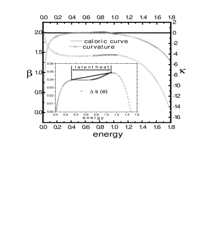
Figure 1: Microcanonical caloric curve $\beta\left(\varepsilon\right)=\partial s\left(\varepsilon\right)/\partial\varepsilon$ and curvature $\kappa\left(\varepsilon\right)=\partial^{2}s\left(\varepsilon\right)/\partial\varepsilon^{2}$ of the $25\times 25$ Potts model with $q=10$ states with periodic boundary conditions obtained by using the GCMMC algorithm. Notice the energetic region with a negative heat capacity. The inserted graph shows the behavior of the relative microcanonical entropy $\Delta s\left(\varepsilon\right)$ in which is remarkable the existence of a convex intruder. Errors are smaller than the symbols linear dimension.

Figure 2: Comparative study between the GCMMC and the Swendsen-Wang (SW) cluster algorithm. The SW algorithm is unable to describe the microcanonical states with a negative heat capacity. Notice the bimodal character of the energy distribution function at $\beta=1.42$.

Notice that the heat capacity $c\left(\varepsilon\right)=-\beta^{2}\left(\varepsilon\right)/\kappa\left(\varepsilon\right)$ becomes negative when $\varepsilon\in\left(\varepsilon_{a},\varepsilon_{b}\right)$ with $\varepsilon_{a}\simeq 0.51$ and $\varepsilon_{b}\simeq 0.93$, which is a feature of a first-order phase transition in a small system becoming extensive in the thermodynamic limit. Such anomalous behavior is directly related with the backbending in the caloric curve $\beta$ versus $\varepsilon$ and the existence of a convex intruder in the relative microcanonical entropy per particle $\Delta s$ versus $\varepsilon$ shown in the inserted graph. This last dependence was obtained from a simple numerical integration of the caloric $\beta\left(\varepsilon\right)$ and curvature $\kappa\left(\varepsilon\right)$ dependences by using the scheme:

$$\delta s\left(\varepsilon\right) =s\left(\varepsilon+\delta\varepsilon\right)-s\left(\varepsilon\right),$$

$$\simeq\beta\left(\varepsilon\right)\delta\varepsilon+\frac{1}{2}\kappa\left(\varepsilon\right)\delta\varepsilon^{2},$$ (48)

based on the second-order approximation of the power expansion of the entropy. We clarify to the reader that the true dependence plotted in this figure is given by $\Delta s^{\ast}\left(\varepsilon\right)=s^{\ast}\left(\varepsilon\right)-s^{\ast}\left(\varepsilon_{\ast}\right)$, where $s^{\ast}\left(\varepsilon\right)=s\left(\varepsilon\right)-\alpha\varepsilon$, with $\varepsilon_{\ast}=0.015$ and $\alpha=1.41$, in order to make more evidence the existence of the convex intruder. It can be shown that the convex intruder disappears progressively with the increasing of the system size until becoming the Maxwell line represented in the inserted graph of the FIG.1, which provides us information about the transition temperature and the latent heat of the first-order phase transition undergone by this model system.

Since the heat capacity is always positive within the canonical ensemble, such anomalous regions are inaccessible in this description. This fact evidences the existence of a significant lost of information about the thermodynamical features of the system during the occurrence of a first-order phase transitions when the canonical ensemble is used instead of the microcanonical one. This difficulty is successfully overcome by the GCMMC algorithm, which is able to predict the microcanonical average of the microscopic observables in these anomalous regions where any others Monte Carlo methods based on the consideration of the Gibbs canonical ensemble such as the original MMC, the Swendsen-Wang and the Wolff single cluster algorithms certainly do not work.

This fact is clearly illustrated in the FIG.2, which evidences that the Swendsen-Wang algorithm is unable to describe the thermodynamic states with a negative heat capacity: its results within the anomalous region differ significantly from the ones obtained by using the GCMMC algorithm. The Swendsen-Wang dynamics exhibits here an erratic behavior originated from the competition of the two metastable states present in the neighborhood of the critical point (the energy distribution function in the canonical ensemble is bimodal when $\beta\in\left(\beta_{1},\beta_{2}\right)$, where $\beta_{1}=1.405$ and $\beta_{2}=1.445$, being this feature the origin of the supercritical slowing down).

As already shown by Gross in ref.gro na , a convex intruder can be associated with the existence of a non-vanishing interphase surface tension during the first-order phase transitions in systems with short-range interactions outside the thermodynamic limit. Nevertheless, we will show in the next subsection that this is not the only one information which could be hidden behind the presence of a negative heat capacity.

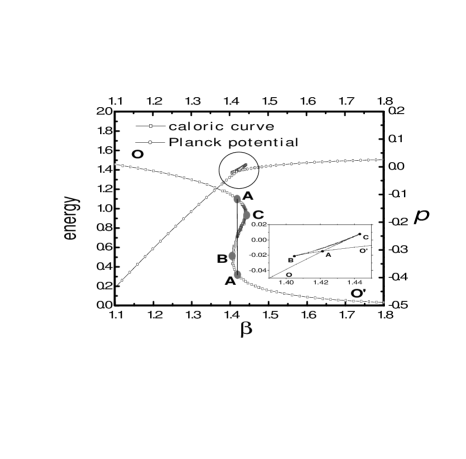
Figure 3: Canonical description of the $q=10$ states Potts model on $25\times 25$ square lattice in which are represented the caloric curve $\varepsilon$ versus $\beta$ and the Planck thermodynamic potential per particles $P$ versus $\beta$ dependences. The inserted graph is a magnification of the region enclosed in the circle indicating the exact point of the first-order phase transition.

We show in FIG.3 the canonical description of this model: the caloric curve and the microcanonical Planck thermodynamic potential per particle $p_{m}\left(\varepsilon\right)$ versus $\beta\left(\varepsilon\right)$ obtained from the Legendre transformation $p_{m}\left(\varepsilon\right)=\beta\left(\varepsilon\right)\varepsilon-s\left(\varepsilon\right)$. The branches OA and AO’ represent the canonically stable thermodynamic states corresponding to the minimal values of the microcanonical Planck potential at a given $\beta$ (the true Planck thermodynamic potential per particle of the canonical description when the system size $N$ is large enough can be approximated by:

$$p_{c}\left(\beta\right)=-\ln Z\left(\beta,N\right)/N\simeq\min_{\beta\left(\varepsilon\right)=\beta}\left\{p_{m}\left(\varepsilon\right)\right\},$$ (49)

being $Z\left(\beta,N\right)$ the canonical partition function). Thus, the points A represent the critical point of the first-order phase transitions where $\beta_{A}\simeq 1.421$, which is recognized from the condition:

$$\text{ }\beta_{A}=\beta\left(\varepsilon_{A}^{\left(-\right)}\right)=\beta\left(\varepsilon_{A}^{\left(+\right)}\right)\text{ and }p\left(\varepsilon_{A}^{\left(-\right)}\right)=p\left(\varepsilon_{A}^{\left(+\right)}\right),$$ (50)

and appreciated in the inserted graph. Obviously, the first derivative of the canonical Planck thermodynamic potential 49 exhibits a discontinuity at $\beta=\beta_{A}$. Since $\varepsilon_{A}^{\left(-\right)}\simeq 1.099$ and $\varepsilon_{A}^{\left(+\right)}\simeq 0.319$, the estimated latent heat $q_{lh}$ associated to this phase-transition is given by $q_{lh}=\varepsilon_{A}^{\left(-\right)}-\varepsilon_{A}^{\left(+\right)}\simeq 0.78$.

The energy distribution function within the canonical ensemble is bimodal inside the interval $\left(\beta_{C},\beta_{B}\right)$ with $\beta_{B}\simeq 1.405$ and $\beta_{C}\simeq 1.443$, which is directly related with the existence of metastable states, the branches AC (supercooled disordered states) and AB (superheated ordered states), which are the origin of the supercritical slowing down behavior observed during the Monte Carlo simulations by using the ordinary Metropolis importance sample algorithm MMC (the exponential divergence of the correlation time with the system size increasing).

The branch BC is canonically unstable since its points represent thermodynamical states with a negative heat capacity associated to the convex intruder of the microcanonical entropy, where $\varepsilon_{B}\simeq 0.933$ and $\varepsilon_{C}\simeq 0.512$. The energy region $\left(\varepsilon_{C},\varepsilon_{B}\right)$ is practically invisible within the canonical description when the system is large enough, and consequently, the ordinary Metropolis algorithm based on the Gibbs ensemble will never access there as a consequence of the ensemble inequivalence. Fortunately, the Metropolis algorithm based on the reparametrization invariance (the using of generalized canonical ensembles) considered in the present study overcomes successfully all those the difficulties undergone by the original method

IV.3 Magnetic properties for $q=10$

The Potts model can be easily rephrased as ferromagnetic system with the introduction of the bidimensional vector variable $\mathbf{s}_{i}=\left[\cos\left(\kappa\sigma_{i}\right),\sin\left(\kappa\sigma_{i}\right)\right]$ with $\kappa=2\pi/q$, where the total magnetization is simply given by $\mathbf{M}=\sum_{i}\mathbf{s}_{i}$. Their magnetic thermostatistical properties will be studied in the present subsection by means of the average magnetization $\left\langle\mathbf{M}\right\rangle$ and the square dispersion $G=\left\langle\left(\mathbf{M}-\left\langle\mathbf{M}\right\rangle\right)^{2}\right\rangle$ which characterizes the fluctuations of this microscopic observable.

It is well-known that the square dispersion of the total magnetization $G$ provides us a measure $g$ about the  spatial correlations between the spin particles

$$g=\frac{G}{N}\equiv\frac{1}{N}\sum_{ij}g_{ij},$$ (51)

where $g_{ij}=\left\langle\mathbf{s}_{i}\cdot\mathbf{s}_{j}\right\rangle-\left\langle\mathbf{s}_{i}\right\rangle\cdot\left\langle\mathbf{s}_{j}\right\rangle$ is the two-point correlation function. This quantity is also related with the magnetic susceptivity $\chi\equiv dM/dB$ of the system under the presence of an external magnetic field $\mathbf{B}$ (coupled to the total magnetization modifying the original Hamiltonian $H$ 47 as follows $H_{B}=H-\mathbf{B}\cdot\mathbf{M}$) throughout the called static susceptibility sum rule Gold :

$$\frac{\partial P}{\partial B}=\beta M,~{}\frac{\partial M}{\partial B}=\beta G_{c},$$ (52)

within the canonical description, while the corresponding identities in the microcanonical ensemble are given by:

$$\frac{\partial S}{\partial B}=\beta M,~{}\frac{\partial M}{\partial B}=\beta G_{m}+M\frac{\partial M}{\partial E},$$ (53)

where $P$ and $S_{B}$ are the Planck potential of the canonical ensemble and the Boltzmann entropy of the microcanonical ensemble respectively, $B\equiv\left|\mathbf{B}\right|$ and $M$ is the projection of the total magnetization along the external magnetic field vector (see demonstration in appendix C).

It is very important to remark that although the existence of the ensemble equivalence in the thermodynamic limit allows us to identify asymptotically the expectation values of the microscopic observables (like the total magnetization $\mathbf{M}$), those quantities characterizing their fluctuations ($G$) and the response functions ($\chi$) depend essentially on the nature of the statistical ensemble used in the description. For example, while the canonical susceptibility is always positive, $\chi_{c}=\beta G_{c}\geq 0$, its corresponding microcanonical quantity $\chi_{m}$ could be negative as a consequence of the presence of the term $M\partial M/\partial E$ in the second relation of the equation 53 since magnetization decreases in the ferromagnetic systems with the energy increasing.

Let us return to the study of the magnetic properties of the Potts model. It is very easy to see that the Hamiltonian 47 is invariant under the discrete group of transformations $\Pi_{q}$ composed by the $q!$ permutations among $q$ spin states. The subgroup of cyclic permutations $Z_{q}=\left\{T_{k};k=1,2,...q\right\}$ is also a subgroup of the group of bidimensional rotations $U\left(2\right)$, whose k-th transformation $T_{k}$ acting on a given vector variable $\mathbf{s}\left(\sigma\right)=\left[\cos\left(\kappa\sigma\right),\sin\left(\kappa\sigma\right)\right]$ induces a rotation in an angle $\Delta\varphi=2\pi k/q$:

$$T_{k}\mathbf{s}\left(\sigma\right)=\mathbf{s}\left(\sigma+k\right).$$ (54)

Obviously, the existence of this last symmetry leads trivially to the vanishing of the exact statistical average of the magnetization.

However, a net magnetization can appears at low energies during the paramagnetic-ferromagnetic phase transition (from disordered states towards the ordered ones) as a consequence of the spontaneous symmetry breaking associated to the nontrivial occurrence of an ergodicity breaking in the underlying dynamical behavior of this model system. This dynamical phenomenon manifests itself when the time averages and the ensemble averages of certain macroscopic observables can not be identified due to the microscopic dynamics is effectively trapped in different subsets of the configurational or phase space during the imposition of the thermodynamic limit $N\rightarrow\infty$ Gold .

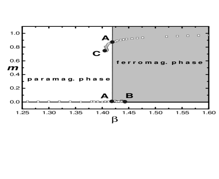
Figure 4: Magnetization $m$ versus $\beta$ dependence o the $q=10$ states Potts model with $L=25$, which shows the existence of a discontinuous ferromagnetic-paramagnetic phase transition at $\beta=\beta_{A}=1.421$.

We show in the FIG.4 the magnetization density $m=\left|\left\langle\mathbf{M}\right\rangle\right|/N$ within the canonical ensemble, where the stable (OA and AO’) and metastable branches (AC and AB) are clearly visible. The existence of a ferromagnetic-paramagnetic phase transition at the critical point $\beta_{A}$ shows clearly that the $Z_{q}$ symmetry has been spontaneously broken. However, it is remarkable how a net magnetization appears abruptly, that is, with a discontinuous character, a behavior which is very similar to the one observed during the solid-liquid first-order phase transition where the traslational symmetry is also spontaneously broken.

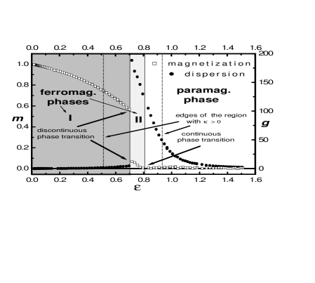
Figure 5: Magnetic properties of the model within the microcanonical ensemble in which is shown the existence of two phase transitions at $\varepsilon_{ff}\simeq 0.7$ (ferro-ferro) and $\varepsilon_{fp}\simeq 0.8$ (ferro-para).

As already commented in the above subsection, there are many thermodynamic information which could be hidden behind a negative heat capacity during the canonical description. Particularly, the reader may agree with us that it is reasonable to expect within the microcanonical description the existence of a critical energy where ferromagnetic-paramagnetic phase transition takes place without the discontinuous character of the magnetization curve observed within the canonical description. Surprisingly, reader can notice that the qualitative behavior of the magnetic properties of this model system shown in the FIG.5 (magnetization density $m$ and the dispersion $g=G/N$) are much more interesting than our preliminary idea.

This magnetization density $m$ versus $\varepsilon$ dependence evidence clearly what could be considered as two phase transitions within the microcanonical description of the $q=10$ states Potts model for $L=25$: a continuous (para-ferro) phase transition at the critical point $\varepsilon_{fp}\simeq 0.8$, and a discontinuous (ferro-ferro) phase transition at $\varepsilon_{ff}\simeq 0.7$. Most of thermodynamic points were obtained from a data of $n=10^{5}$ Metropolis iterations, with the exception of all those points belonging to the energetic interval $\left(0.7,0.93\right)$ where $n=5\times 10^{6}$ iterations were needed in order to reduce the significant dispersion of the expectation values close to the critical points. The large dispersions observed throughout the dispersion $g$, the large relaxation times during the Metropolis dynamics, and the qualitative behavior of the magnetization density strongly suggest us the presence of several metastable states with different magnetization states at a given energy within this last region, which is demonstrated in the FIG.6.

Figure 6: Histogram of the projection of the microscopic magnetization along the direction of the spontaneous magnetization of the ferromanet type I, which demostrates the existence of metastable states when $\varepsilon=0.844$.

The microcanonical continuous phase transition between the paramagnetic-ferromagnetic type I  (with low magnetization density) phases takes place with the spontaneous breaking of the $Z_{q}$ symmetry associated to the occurrence of an ergodicity breaking in the microscopic dynamics. Apparently, the large fluctuations and long-range correlations ordinarily associated to this kind of phase transition are overlapped with the large fluctuations associated to the existence of metastable states.

On the other hand, the $Z_{q}$ symmetry has been already spontaneously broken during the occurrence of the microcanonical discontinuous phase transition between the ferromagnet type I - ferromagnet type II  (with high magnetization density). However, this phase transition is also associated to the occurrence of an ergodicity breaking in the underlying microscopic picture: the microscopic dynamics of this model system can be effectively trapped in the thermodynamic limit $L\rightarrow\infty$ in any of the metastable states with different magnetization density present in the neighborhood of this critical point.

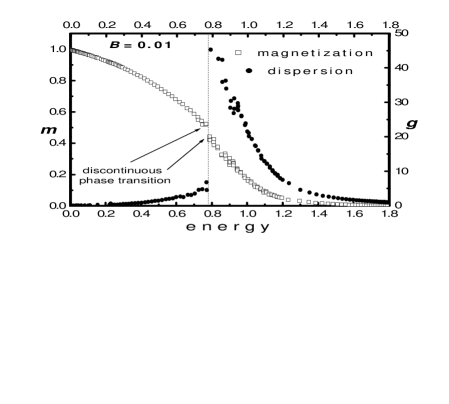
Figure 7: Magnetic properties of the model under the presence of an external magnetic field with $B=0.01$. Notice that in this case the dispersion is not large than in the first case with $B=0$, but it is clearly visible the existence of the ferromagnetic-paramagnetic phase transition.

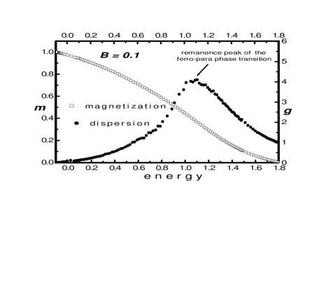
Figure 8: The same dependences of the FIGs (5) and (7), but now under the influence of an external magnetig field with $B=0.1$.

The FIGs 7 and 8 show the magnetic properties of the model system under the presence of an external magnetic field with $B=0.01$ and $B=0.1$. The reader can notice in the FIG.7 that the microcanonical discontinuous phase transition is also present for low intensities of the external magnetic field, but the discontinuity observed in the magnetization $m\left(\varepsilon\right)$ and the dispersion $g\left(\varepsilon\right)$ dependences is not so abrupt in this case. Apparently, such behavior is reduced progressively with the $B$ increasing until disappear when the magnetic field intensity is large enough, as already illustrated in the FIG.8. This last figure shows that the dispersion curve has a peak, which is a remanence of the paramagnetic-ferromagnetic phase transition when $B\not=0$. Reader may notice that the presence of discontinuous phase transition affects significantly the qualitative behavior of the square dispersion $g$ of the magnetization.

IV.4 What can be learned from the microcanonical description of this model system?

The backbending behavior in the microcanonical caloric curve shown in the FIG.1 (becoming a plateau in the thermodynamic limit) is usually interpreted as the signature of a first-order phase transition (with spontaneous symmetry breaking). On the other hand, the magnetization curve shown in the FIG.5 exhibits two anomalies which can be also considered as phase transition of the thermostatistical description of this model system: a continuous phase transition (with spontaneous symmetry breaking) and a discontinuous phase transition (where the underlying symmetry has been already broken). Consequently, what kind of phase transition exhibits the thermostatistical description of the $q=10$ states Potts model? The answer of the above question in our viewpoint depends on the external conditions imposed to the system.

Obviously, this model system put in contact with a Gibbs thermostat undergoes a discontinuous first order phase transition while a smooth change of the inverse temperature $\beta$ in the neighborhood of the critical point $\beta_{A}=1.421$. There, the phase coexistence phenomenon characteristic of this kind of phase transitions can be observed and the region $\left(\varepsilon_{C},\varepsilon_{B}\right)$ is inaccessible within the Gibbs canonical description in the thermodynamic limit.

A different picture is revealed when the model system is isolated (microcanonical description). All the anomalous region $\left(\varepsilon_{C},\varepsilon_{B}\right)$ is now accessible. Many microcanonical states there show no anomalous behavior with the exception of those macrostates within the region $\left(\varepsilon_{ff},\varepsilon_{B}\right)$ which are affected by the incidence of metastable states. The imposition of the thermodynamic limit leads to the suppression of the metastable states, but the existence of anomalous behaviors persists in the neighborhood of the para-ferro continuous phase transition at $\varepsilon_{fp}$ and the ferro-ferro discontinuous phase transition at $\varepsilon_{ff}$. Interestingly, such anomalies can not be apparently associated with any anomaly of the caloric or curvature curves in the FIG.1, but by using the microcanonical magnetization curve shown in FIG.5.

Taking into account the microcanonical thermodynamic identities in the thermodynamic limit $N\rightarrow\infty$ shown in the equation 53 between the entropy $S$, the magnetization $M$, the external magnetic field $B$ and the square dispersion $G$: the discontinuous phase transition at $\varepsilon_{ff}$ corresponds to a discontinuity of the first derivative of the entropy per particle:

$$\lim_{\varepsilon\rightarrow\varepsilon_{ff}^{+}}\lim_{B\rightarrow 0}\frac{\partial s\left(\varepsilon,B\right)}{\partial B}\not=\lim_{\varepsilon\rightarrow\varepsilon_{ff}^{-}}\lim_{B\rightarrow 0}\frac{\partial s\left(\varepsilon,B\right)}{\partial B},$$ (55)

while the continuous phase transition at $\varepsilon_{fp}$ corresponds to a discontinuity of the second derivative of the entropy:

$$\lim_{\varepsilon\rightarrow\varepsilon_{fp}^{+}}\lim_{B\rightarrow 0}\frac{\partial^{2}s\left(\varepsilon,B\right)}{\partial\varepsilon\partial B}\not=\lim_{\varepsilon\rightarrow\varepsilon_{fp}^{-}}\lim_{B\rightarrow 0}\frac{\partial^{2}s\left(\varepsilon,B\right)}{\partial\varepsilon\partial B}.$$ (56)

Consequently, the present microcanonical anomalies can be recognized by the lost of analyticity of the entropy per particle in the thermodynamic limit, and the same ones are related with the occurrence of an ergodicity breaking in the microscopic picture of this model system.

V Towards a new classification scheme

The analysis developed in the above two sections allows us to classify the thermodynamic anomalies type A and type B introduced in the beginning of the section III as follows. The anomaly type A are just anomalies observed in open systems (canonical description) which are dependent on the external experimental conditions due to they originated from the ensemble inequivalence. The anomaly type B are all those anomalies which are always observed in an isolated system (microcanonical description) and can potentially appear under any external experimental conditions.

V.1 The anomalies type A

Anomalies type A correspond what we usually called as first-order phase transitions in conventional Thermodynamics, and they are only relevant for an open system since their existence depends crucially on the nature of the external conditions imposed to the interest system. We recognized them by the existence of a latent heat for the phase transition associated to the multimodal character (a signature of the phase coexistence) of the energy distribution function within the (generalized) canonical description. In terms of the thermodynamic potentials, an anomaly type A manifests as a discontinuity in some of the first derivatives the generalized Planck potential, which are directly related to the existence of convex regions of the microcanonical entropy $S$ in a given reparametrization $\Theta$ dependent on the external experimental setup (the using of a generalized thermostat).

An anomaly type A represents in this way the inability of the (generalized) canonical description in describing all those macrostates which can be accessed within the microcanonical description. As already shown, this kind of anomaly can be avoided by using another experimental setup which ensures the global equivalence of the generalized canonical description with the microcanonical ensemble. The Monte Carlo method exposed in the subsection III.4 is precisely based on this idea.

The Swensen-Wang algorithm is a Monte Carlo cluster algorithm based on the consideration of the Gibbs canonical ensemble, that is, it simulates the thermodynamical equilibrium of the Potts model system put in contact with an ordinary thermostat (heat bath). Since the Gibbs canonical description of the $q=10$ states Potts model is not globally equivalent to its microcanonical description, a sudden change in the energy per particle $\varepsilon$ of this model system is observed in the neighborhood of the critical inverse temperature $\beta_{c}\simeq 1.421$. On the other hand, the GCMMC algorithm describes the thermodynamic equilibrium of a given system in contact with a generalized thermostat. As already shown in FIG.2, this change of the external conditions allows the system to access to all those inaccessible regions within the Gibbs canonical ensemble, and therefore, neither there exist lost of information nor any sudden change of the energy per particle is observed now. Thus, the thermodynamical study of the $q=10$ states Potts model shows that the first-order phase transitions are avoidable thermodynamical anomalies.

V.2 The anomalies type B

The lost of analyticity of the entropy per particle in the thermodynamic limit, the anomaly type B, is obviously the only one mathematical anomaly of the microcanonical entropy which is reparametrization invariant. This character explains why this kind of anomaly could potentially appear under any external experimental setup (which determines the specific reparametrization $\Theta$ used in the generalized canonical ensemble), and consequently, it is the only thermodynamical anomaly microcanonically relevant. We say ”potentially” because of there exists the possibility that an anomaly type B could be hidden by the lost of information associated to the ensemble inequivalence, i.e.: the continuous (ferro-para) and the discontinuous (ferro-ferro) phase transitions described in the FIG.5 are hidden within the Gibbs canonical description.

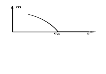
Figure 9: Schematic representation of the onset of the magnetization curve within the microcanonical description in the limit of zero applied magnetic field of a ferro-para phase transition.

Since the microcanonical ensemble is just a dynamical ensemble, the anomaly type B should be the macroscopic manifestation of a sudden change in the dynamical behavior of the isolated Hamiltonian system. As already pointed in our study of the $q=10$ states Potts model, the lost of analyticity of the entropy per particle in the thermodynamic limit seems to be related to the ergodicity breaking phenomenon. The well-known spontaneous symmetry breaking associated to the ferro-para second order phase transitions schematically represented in the FIG.9 is a generic example of an ergodicity breaking which is always connected to a lost of analyticity of the entropy per particle in the thermodynamic limit. The demonstration starts from the consideration of the first identity of the equation 53:

$$\frac{\partial s\left(\varepsilon,B\right)}{\partial B}=\beta\left(\varepsilon,B\right)m\left(\varepsilon,B\right),$$ (57)

which allows us to obtain the magnetization curve $m\left(\varepsilon,B\right)$ from the entropy per particle in the thermodynamic limit $s\left(\varepsilon,B\right)$, being $\beta\left(\varepsilon,B\right)=\partial s\left(\varepsilon,B\right)/\partial\varepsilon$ the microcanonical caloric curve. The partial derivative $\partial/\partial\varepsilon$ of the above equation is given by:

$$\frac{\partial^{2}s\left(\varepsilon,B\right)}{\partial\varepsilon\partial B}=\frac{\partial\beta\left(\varepsilon,B\right)}{\partial\varepsilon}m\left(\varepsilon,B\right)+\beta\left(\varepsilon,B\right)\frac{\partial m\left(\varepsilon,B\right)}{\partial\varepsilon}.$$ (58)

While the first derivative of the caloric curve $\partial\beta\left(\varepsilon,B\right)/\partial\varepsilon$ always exists in short-range interacting systems, the dependence $\partial m\left(\varepsilon,B\right)/\partial\varepsilon$ exhibits a discontinuity at the critical point $\varepsilon_{c}$ in the limit of zero applied magnetic field, and consequently:

$$h\left(\varepsilon\right)=\lim_{B\rightarrow 0}\frac{\partial^{2}s\left(\varepsilon,B\right)}{\partial\varepsilon\partial B}$$ (59)

is discontinuous function.

The anomaly type B described above can be referred as a microcanonical continuous phase transition since the first derivatives of the entropy per particle in the thermodynamic limit are continuous (Anomaly type B.I). Contrary, we can referred a anomaly type B as a microcanonical discontinuous phase transition when some of the first derivatives of the entropy per particle in the thermodynamic limit are discontinuous at the point of lost of analyticity (Anomaly type B.II). Particularly, the ferro-ferro phase transition observed in the microcanonical description of the $q=10$ states Potts model is a clear example of a microcanonical discontinuous phase transition: Since the magnetization curve is discontinuous, and therefore, the first derivative 57 is also discontinuous.

The reader can notice that most of the well-known continuous (second-order) phase transitions in the conventional Thermodynamics corresponds to microcanonical continuous phase transitions, since the applicability of the Legendre transformation $P=\beta E-S$ during the ensemble equivalence in the thermodynamic limit allows that every anomaly type B.I leads to lost of analyticity of the Planck potential (or the Helmholtz free energy). However, we will show below that all anomaly that could be classified as a continuous phase transition within the conventional Thermodynamics does not correspond necessarily to a microcanonical continuous phase transition.

A feature of the physical systems exhibiting a continuous phase transition associated to the occurrence of an spontaneous symmetry breaking is the existence of divergent power laws behavior in the heat capacity (and other response functions) in the neighborhood of the critical point $\beta_{c}$:

$$c\left(\beta\right)=\left\{\begin{array}[c]{cc}A^{\left(-\right)}\left(-t\right)^{-\alpha}&t<0,\\ A^{\left(+\right)}t^{-\alpha}&t>0,\end{array}\right.$$ (60)

being $t=\beta_{c}-\beta$, where the called critical exponent $\alpha$ and the amplitude ratio $A^{\left(+\right)}/A^{\left(-\right)}$ are the same within a universality class Gold . The characteristic ”$\lambda$-form” of the continuous phase transitions is directly related to the presence of divergent power laws with universal ratio $A^{\left(+\right)}/A^{\left(-\right)}\not=1$ and nontrivial critical exponent $\alpha$: i.e.: $\alpha=\left(0.110-0.116\right)$ for the Ising universality class. The divergence of the heat capacity in the continuous phase transitions can be explained by an eventual vanishing of the second derivative of the entropy $\partial^{2}s/\partial\varepsilon^{2}$ at the critical point. However, the nature of the divergent power law depends crucially on the analyticity of the entropy per particle in the thermodynamic limit.

Let be a hypothetical system whose entropy per particle in the thermodynamic limit $s\left(\varepsilon\right)$ is analytical in a given region but its second derivative $\partial^{2}s\left(\varepsilon\right)/\partial\varepsilon^{2}$ vanishes eventually at a certain point $\varepsilon_{c}$ of this region. This is just anomaly type A where the anomalous region of the microcanonical entropy is composed by only one point. Since the caloric curve $\beta\left(\varepsilon\right)=\partial s\left(\varepsilon\right)/\partial\varepsilon$ is bijective in this case, ensemble equivalence is ensured. However, the average square dispersion of the system energy and the heat capacity within the Gibbs canonical ensemble go to infinite at $\varepsilon_{c}$, so that, the second derivative of the Planck thermodynamic potential diverges at the corresponding critical point $\beta_{c}=\beta\left(\varepsilon_{c}\right)$. In spite of the present anomalous behavior can be classified as a continuous phase transition in the conventional Thermodynamics viewpoint, it does not correspond to any microcanonical phase transition. Particularly, the missing of the lost of analyticity of the entropy allows us to think that the above anomaly can not be associated to the occurrence of an ergodicity breaking. For example, the analytical character of the entropy per particle in the thermodynamic limit of the above hypothetical system allows us to approximate the caloric curve $\beta\left(\varepsilon\right)$ in the neighborhood of the critical point $\varepsilon_{c}$ by the Taylor power series:

$$\beta=\beta_{c}-\lambda\left(\varepsilon-\varepsilon_{c}\right)^{2n+1}+...,$$ (61)

where $\lambda>0$ and $n$ a positive integer, expression leading to a power law divergent behavior of the heat capacity 60 with critical exponent $\alpha=2n/\left(2n+1\right)$ and $A^{\left(-\right)}=A^{\left(+\right)}=\beta_{0}^{2}/\lambda^{1-\alpha}\left(2n+1\right)$. Consequently, this result corresponds to a critical phenomenon with universal ratio $A^{\left(+\right)}/A^{\left(-\right)}\equiv 1$ and critical exponent $\alpha$ related to a odd number $2n+1=1/\left(1-\alpha\right)$.

The above result allows to claim that the existence of divergent power laws with nontrivial critical exponents $\alpha$ and universal ratio $A^{\left(+\right)}/A^{\left(-\right)}\not=1$ in most of real physical systems exhibiting a continuous phase transition associated to the occurrence of a spontaneous symmetry breaking is a clear indicator of the lost of analyticity of the entropy per particle in the thermodynamic limit in such cases. An anomaly like the one exhibited by our hypothetical system can be seen as an asymptotic case of a discontinuous phase transition, which shall be referred in this work as a 1st-kind continuous phase transition.

The discontinuous character of the first derivatives of the entropy per particle in the thermodynamic limit during the occurrence of the microcanonical discontinuous phase transitions can lead to discontinuity of some of the first derivatives of the Planck potential (or other thermodynamic potential characterizing an open system) or even provoke the discontinuity of the thermodynamical potential itself. This last mathematical anomaly is unusual for the systems dealt within the conventional Thermodynamics, but it can be observed in the astrophysical context and others long-range interacting systems. The interested reader can find in the ref.chava an example of a discontinuity of the caloric curve $\beta\left(\varepsilon\right)$ observed in the thermodynamical description of astrophysical model, indicating the existence of metastable states at the same total energy with different temperature (mathematical anomaly leading to a discontinuity of the Planck potential $P=\beta E-S$). While the thermodynamical behavior associated to the discontinuity of the Planck thermodynamic potential could be referred as a zero-order phase transition within the well-known Ehrenfest classification, the discontinuity of some of its first derivatives is just a discontinuous phase transition.

Although we can not provide in this work a rigorous demonstration about the relationship between the lost of analyticity of the entropy per particle in the thermodynamic limit with the occurrence of ergodicity breaking in the microscopic dynamics, we have considered in this work some examples suggesting that such connection exists. Loosely speaking, the ergodicity breaking takes place as a consequence of the dynamical competition among metastable states, where the predominance of any of them depends crucially on the initial conditions of the microscopic dynamics and the boundary conditions gallavotti ; Gold . Particularly, the thermodynamical study of the $q=10$ states Potts model presented in the section IV suggests that the microcanonical continuous phase transition observed in this model system is provoked by the competition among metastable states which essentially identical (states with the same magnetization density) since they are related by a symmetry transformation ($Z_{q}$). On the other hand, the microcanonical discontinuous phase transition observed in this model system is also provoked by the competition among metastable states, which are essentially different (states with different spontaneous magnetization density) since them can not be related by a symmetry transformation.

The reader may notice that the discontinuity of the first derivative of the entropy described in the ref.chava (a microcanonical discontinuous phase transition) can be associated to the occurrence of ergodicity breaking originated from the competition among metastable states with different temperature.

V.3 Summary

As already shown in this work, the existence and the features of anomalies observed in the thermodynamical description of given Hamiltonian system depends crucially on the external conditions which have been imposed. It means that a phase transition is not only an intrinsic thermodynamical anomaly of a given system, but also a specific response to the nature of the external control of its thermodynamic equilibrium. Generally speaking, the mathematical description of the phase transitions for systems in thermodynamic limit starts from the consideration of the lost of analyticity of the thermodynamic potential which is relevant in a given application.

The most simple characterization of the thermodynamical anomalies of a given Hamiltonian system is obtained within the microcanonical description, which is relevant when the interest system is isolated. Phase transitions here can be recognized by the lost of analyticity of the entropy $S$ in the thermodynamic limit, a mathematical anomaly (type B.I or B.II) which is reparametrization invariant and should be originated from the occurrence of the ergodicity breaking phenomenon. This results are summarized in the Table 1.

Thermodynamical anomaly	Classification
$\begin{array}[c]{l}\text{Type {A} (presence of non }\\ \text{concave regions of the entropy }S\text{)}\\ \text{(non reparametrization invariant)}\end{array}$	microcanonically irrelevant
$\begin{array}[c]{c}\text{Type {B.I} (lost of analyticity of }\\ \lx@intercol\text{the entropy }S\text{\ with continuous}\hfil\lx@intercol\\ \lx@intercol\text{ first derivatives) }\hfil\lx@intercol\\ \lx@intercol\text{(reparametrization invariant)}\hfil\lx@intercol\end{array}$	microcanonical continuous PT
$\begin{array}[c]{c}\text{Type {B.II} (lost of analyticity of }\\ \lx@intercol\text{the entropy }S\text{ with some}\hfil\lx@intercol\\ \lx@intercol\text{discontinuous first derivatives)}\hfil\lx@intercol\\ \lx@intercol\text{(reparametrization invariant)}\hfil\lx@intercol\end{array}$	microcanonical discontinuous PT

Table 1: Phase transitions (PT) within the microcanonical description (isolated system).

The presence of the experimental setup controlling the thermodynamic equilibrium of the interest system leads to a significant complexation of the phase transitions. Phase transitions here are recognized by the lost of analyticity of the relevant thermodynamic potential $\mathcal{P}$ (Planck or Helmholtz free energy, gran potential or any other admissible generalization).

We have now five thermodynamical anomalies for the open systems in contract to the only two relevant when they are isolated. Besides the introduction of the zero-order phase transitions, we consider also a distinction among those continuous and discontinuous phase transitions which are related with a lost of analyticity of the entropy $S$. A tentative classification scheme is summarized in the Table 2.

Thermodynamical anomaly	Classification
$\begin{array}[c]{l}\mathcal{P}\text{ is discontinuous as consequence}\\ \text{of a discontinuity of control parame }\\ \text{ter }\eta=\partial S/\partial I\text{ used in the Legendre }\\ \text{transformation }\mathcal{P}=\eta I-S\text{.}\end{array}$	zero-order PT
$\begin{array}[c]{l}\text{Some of first derivatives of }\mathcal{P}\text{ are }\\ \text{discontinuous as consequence of }\\ \text{the ensemble inequivalence.}\end{array}$	1st-kind discontinuous PT
$\begin{array}[c]{l}\text{Some of first derivatives of }\mathcal{P}\text{ are}\\ \text{discontinuous as consequence of }\\ \text{a discontinuity in some of the first }\\ \text{derivatives of the entropy }S\text{.}\end{array}$	2st-kind discontinuous PT
$\begin{array}[c]{l}\text{Lost of analyticity of }\mathcal{P}\text{ with con-}\\ \text{tinuous first derivatives without }\\ \text{a lost of analyticity of entropy }S\text{.}\end{array}$	1st-kind continuous PT
$\begin{array}[c]{l}\text{Lost of analyticity of }\mathcal{P}\text{ with con-}\\ \text{tinuous first derivatives associated }\\ \text{to a lost of analyticity of entropy }S\text{.}\end{array}$	2st-kind continuous PT

Table 2: Tentative classification scheme of the phase transitions (PT) within a ”canonical description” (open system).

Finally, the Table 3 summarizes the ”genealogy” of the phase transitions associated to the mathematical anomalies type A and B of the microcanonical entropy $S$ which were described in the present section. While the anomaly type A (non concavity of $S$ in a given reparametrization $\Theta$) is irrelevant when the interest system is isolated, the incidence of certain experimental setup turns this behavior in a lost of analyticity of the relevant thermodynamical potential $\mathcal{P}$ associated with the ensemble inequivalence (a 1st-kind discontinuous PT or its limiting case: 1st–kind continuous phase transition). Type B anomalies always leads to the lost of analyticity of $\mathcal{P}$ whenever they are not hidden by the ensemble inequivalence. The corresponding phase transitions are always originated from the occurrence of ergodicity breaking. While microcanonical continuous phase transitions are directly related to the 2st-kind continuous phase transitions, a microcanonical discontinuous phase transitions can manifest as a zero-order phase transition or a 2st-kind discontinuous phase transition.

Anomaly	Isolated system	Open system
Type A	microcanonically irrelevant	1st-kind discont. PT 1st-kind cont. PT
Type B.I	micro. continuous PT	2st-kind cont. PT
Type B.II	micro. discontinuous PT	zero-orden PT 2st-kind discont. PT

Table 3: Genealogy between the thermodynamic anomalies type A an B under different external conditions.

VI Conclusions

We have shown in the section II that the microcanonical description is characterized by the presence of an internal symmetry whose existence is closely related to the dynamical origin of this ensemble: the reparametrization invariance. Such symmetry leads naturally to a new geometric formalism of the Thermodynamics within the microcanonical ensemble which is not based on the consideration of a Riemannian metric derived from the Hessian of the microcanonical entropy like other thermodynamic formalisms proposed in the past rupper .  While the microcanonical entropy becomes a scalar function within the present geometrical framework, we show that its convex or concave character depends on the reparametrization of the integrals of motion which are relevant for the microcanonical description. Such ambiguity leads necessarily to a reconsideration of any classification scheme of the phase transitions based on the concavity of the microcanonical entropy gro1 .

Sections III-V were devoted to carry out a tentative analysis of the above question. Interestingly, this aim demands a necessary and unexpected generalization of the Gibbs canonical ensemble and the classical fluctuation theory where the reparametrization invariance introduced in the section II plays a more fundamental role than in the conventional Thermodynamics. While reparametrization changes do not alter the microcanonical description, such transformations represent specific substitutions of the external experimental setup leading to different generalized canonical descriptions 28 for the open system. Particularly, we have shown that the well-known ensemble inequivalence of the Gibbs canonical ensemble 18 can be avoided within an appropriate generalized canonical ensemble 28, which describes an open system put in contact with a generalized version of the Gibbs thermostat (heat bath) whose inverse temperature $\beta$ exhibits correlated fluctuations with the fluctuations of the total energy $E$ of the interest system (see in subsection III.3). This feature of the generalized canonical ensemble put the basis for an unexpected generalization of the classical fluctuation theory rupper where the inverse temperature of the generalized thermostat $\beta$ and the total energy of the interest system $E$ behave as complementary thermodynamic quantities and the convex regions derived from the entropy Hessian admit a simple interpretation: there the inverse temperature $\beta$ can not be fixed since $\left\langle\delta\beta\delta E\right\rangle\geq 1$ (see in subsection III.5). The analysis of such questions demands a further study. Particularly, we have only consider in the present work a generalization of the Gibbs canonical ensemble, while it is reasonable a generalization of any Boltzmann-Gibbs distributions.

The possibility of avoid the ensemble inequivalence by using the generalized canonical ensemble 28 allows us to improve some Monte Carlo methods based on the consideration of the Gibbs canonical ensemble. This aim was carried out in the subsection III.4 and the ref.vel-mmc as a example of application of the present reparametrization invariance ideas for the implementation of a generalized version of the well-known Metropolis importance sample algorithm met .

The most important conclusion obtained from our subsequent analysis is the recognition about the fundamental role of the arbitrary external conditions (the using of different experimental setups) which can be imposed to the interest system in order to control its thermodynamic equilibrium. Particularly, the existence and nature of the phase transitions (admitting them as a sudden change of the thermodynamic behavior of a given system while a smooth change of a control parameter) depends crucially on the nature of the external experimental setup. This fact was shown in the section IV by considering the microcanonical description of the $q=10$ states Potts model system, where the Gibbs canonical description predicts the occurrence of a first-order phase transition and the microcanonical description exhibits two microcanonical phase transitions which are hidden by the ensemble inequivalence.

While there are only two thermodynamical anomalies which can be classified as phase transitions within the microcanonical ensemble (presumably associated to the occurrence of ergodicity breaking phenomenon Gold ), there are five of them in an open system (”within a generalized canonical description”): two of them closely related with the ensemble inequivalence (1st-kind discontinuous PT and its limiting case, the 1st-kind continuous PT) and the other three with the lost of analyticity of the entropy $S$ in the thermodynamic limit (zero-order PT, 2st-kind discontinuous PT and the 2st-kind continuous PT). To our viewpoint the present classification scheme is only tentative and also deserves a further analysis of some paradigmatic models as well as the revision of the available literature.

Appendix A Riemannian metric from the Hessian of entropy

Ruppeiner in ref.rupper considers a subsystem $\sigma$ of a larger closed system $\Sigma$ in a thermodynamic equilibrium characterized by the macroscopic parameters $x_{0}$ ( a system + its environment - a situation schematically represented in FIG.10). The probability that the subsystem $\sigma$ be in a the macrostate characterized by the parameters $x$, whose values are enclosed in the range $\left(x,x+dx\right)$ is given by:

$$P\left(x\left|x_{0}\right.\right)dx=\frac{1}{W\left(x_{0}\right)}\Omega\left(x,x_{0}\right)dx,$$ (62)

being $\Omega\left(x,x_{0}\right)$ the density of states at the configuration, and $W\left(x_{0}\right)=\int\Omega\left(x,x_{0}\right)dx$, the total number of microstates of the closed system. Instead of using the Boltzmann entropy associated to the closed system $\Sigma$, $S_{B}\left(x_{0}\right)=\ln W\left(x_{0}\right)$, this author deals with the ”entropy” $S_{0}\left(x,x_{0}\right)=\ln\Omega\left(x,x_{0}\right).$

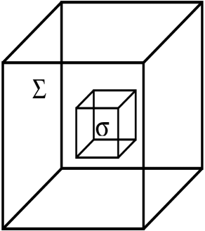
Figure 10: Usual setup in classical thermodynamics fluctuation theory and the canonical ensembles in Statistical Mechanics: a subsystem $\sigma$ of a larger closed enviroment $\Sigma$, which are ordinarily regarded as uniform systems.

The most probable macroscopic configuration $x_{m}$ of the subsystem $\sigma$ can be derived as a solution of the stationary conditions:

$$\frac{\partial S_{0}\left(x_{m},x_{0}\right)}{\partial x^{\mu}}=0,$$ (63)

which ensures the nonnegative definition of the matrix $g_{\mu\nu}$ defined from the Hessian :

$$g_{\mu\nu}\left(x_{0}\right)=-\frac{1}{V}\frac{\partial^{2}S_{0}\left(x_{m},x_{0}\right)}{\partial x^{\mu}\partial x^{\nu}}.$$ (64)

The matrix 64 is invariant under ”reparametrizations” of the thermodynamic parameters $x$ of the subsystem $\sigma$, $y=y\left(x\right)$, since the second terms of the transformation rule:

$$\frac{\partial^{2}S_{0}\left(x\left(y\right),x_{0}\right)}{\partial y^{\alpha}\partial y^{\beta}} =\frac{\partial x^{\mu}}{\partial y^{\alpha}}\frac{\partial x^{\nu}}{\partial y^{\beta}}\frac{\partial^{2}S_{0}}{\partial x^{\mu}\partial x^{\nu}}+\frac{\partial^{2}x^{\mu}}{\partial y^{\alpha}\partial y^{\beta}}\frac{\partial S_{0}}{\partial x^{\mu}},$$

$$\Rightarrow g_{\alpha\beta}\left(x_{0}\right)=\frac{\partial x^{\mu}}{\partial y^{\alpha}}\frac{\partial x^{\nu}}{\partial y^{\beta}}g_{\mu\nu}\left(x_{0}\right)$$ (65)

vanish as a consequence of the stationary conditions 63. This feature allows to take the matrix $g_{\mu\nu}$ as a Riemannian metric which provides important information about the fluctuations around the most probable macroscopic configurations of the subsystem $\sigma$. The reader can compare the result 65 with the one expressed in the equation 15 in order to convince himself that the entropy Hessian of an isolated system is not a Riemannian tensor.

Appendix B Coarsed grained microcanonical entropy

For practical purposes, the Boltzmann entropy $S_{B}=\ln W$ can be estimated by the coarsed grained entropy $S_{\varepsilon}=\ln\left\{\Omega\left(E,N\right)\delta\varepsilon_{0}\right\}$ where $\delta\varepsilon_{0}$ is a very small energy constant which defines certain coarsed grained partition $\mathcal{P}_{\varepsilon}$ of the phase space $\Gamma$. The entropy in other reparametrization $\Theta\left(E\right)=N\varphi\left(E/N\right)$ could be estimated by $S_{\varphi}\left(\Theta,N\right)=\ln\left\{\Omega\left(\Theta,N\right)\delta\varphi_{0}\right\}\,$, where the small constant $\delta\varphi_{0}$ defines another coarsed grained partition $\mathcal{P}_{\varphi}$ of the phase space. Obviously, the entropy estimates $S_{\varepsilon}$ and $S_{\varphi}$ are not equal since the partitions $\mathcal{P}_{\varepsilon}$ and $\mathcal{P}_{\varphi}$ are essentially different. Taking into consideration the transformation rule

$$\Omega\left(\Theta,N\right)=\left|\frac{\partial\Theta}{\partial E}\right|^{-1}\Omega\left(E,N\right),$$ (66)

the absolute discrepancy $\delta S$:

$$\delta S=S_{\varphi}\left(\Theta,N\right)-S_{\varepsilon}\left(E,N\right)=-\ln\left\{\frac{\delta\varepsilon_{0}}{\delta\varphi_{0}}\frac{\partial\varphi\left(\varepsilon\right)}{\partial\varepsilon}\right\}$$ (67)

depends on the relative energy $\varepsilon=E/N$, but the relative discrepancy:

$$\frac{\delta S}{S}\sim\frac{1}{N}\text{ with }S=\frac{1}{2}\left[S_{\varepsilon}+S_{\varphi}\right],$$ (68)

drops to zero in the thermodynamic limit $N\rightarrow\infty$ as consequence of the extensive character of the entropy when $N$ is large enough.

The above reasonings allows us to consider the coarsed grained entropy, or more exactly, the entropy per particle in the thermodynamic limit:

$$s\left(\varepsilon\right)=\lim_{N\rightarrow\infty}\frac{S\left(\varepsilon N,N\right)}{N}=\lim_{N\rightarrow\infty}\frac{S\left(\Theta\left(\varepsilon N\right),N\right)}{N}=s\left(\varphi\right)$$

as a continuous scalar function whose form is independent from the nature of the coarsed grained partitions $\mathcal{P}_{\varepsilon}$ and $\mathcal{P}_{\varphi}$ whenever their respective volume constants $\delta\varepsilon_{0}$ and $\delta\varphi_{0}$ be small enough. Thus, we can assume along the present work the approximation $S\left(E,N\right)\cong S\left(\Theta,N\right)$.

Appendix C Others covariant quantities derived from the Boltzmann entropy

Let us suppose that the integrals of motion depend on certain external parameter $a$, $\hat{I}_{a}=\hat{I}\left(X;a\right)$. By taking the partial derivative of the relation:

$$\Omega\left\langle\hat{O}\right\rangle=\int dX~{}\hat{O}\left(X\right)\delta\left[I-\hat{I}\left(X;a\right)\right],$$ (69)

we obtain the identity:

$$\frac{1}{\Omega}\frac{\partial}{\partial a}\left\{\Omega\left\langle\hat{O}\right\rangle\right\}=\frac{1}{\Omega}\frac{\partial}{\partial I^{S}}\left\{\Omega\left\langle\hat{O}\hat{F}_{a}^{S}\right\rangle\right\},$$ (70)

where the microscopic quantity $\hat{F}_{a}^{S}=\hat{F}_{a}^{S}\left(X;a\right)$ represents the k-th component of the generalized force associated to the parameter $a$:

$$\hat{F}_{a}^{S}=-\frac{\partial\hat{I}_{a}^{S}}{\partial a},$$ (71)

It is very easy to verify that the expectation values $\upsilon^{S}=\left\langle\hat{O}\hat{F}_{a}^{S}\right\rangle$ correspond to the components of a contravariant vector because of they obey to the transformation rule:

$$\upsilon^{\prime K}=\frac{\partial\varphi^{K}}{\partial I^{S}}\upsilon^{S}.$$ (72)

The differential operator:

$$\mathcal{D}\left(\mathbf{u}\right)=\frac{1}{\Omega}\frac{\partial}{\partial I^{S}}\left\{\Omega u^{S}\right\},$$ (73)

is just a linear transformation becoming a contravariant vector field $\mathbf{u}=\left\{u^{S}\right\}$ in a scalar function.

The invariant volume element $d\mu_{g}$ in the Riemannian geometry is derived from the metric $g_{\mu\nu}$ as follows: $d\mu_{g}=\sqrt{g}d^{n}x$, where $\sqrt{g}\equiv\sqrt{\left|\det g_{\mu\nu}\right|}$. The divergence of a given vectorial field $\mathbf{u}$ in this framework is given by:

$$\operatorname*{div}\mathbf{u}=\frac{1}{\sqrt{g}}\frac{\partial}{\partial x^{\mu}}\left\{\sqrt{g}u^{\mu}\right\}.$$ (74)

The analogy between the invariant volume elements $d\mu_{g}=\sqrt{g}d^{n}x\sim d\mu=\Omega dI$ allows us to consider the differential operator $\mathcal{D}\left(\mathbf{u}\right)$ 73 as the divergence of a contravariant vector field. Thus, it is obvious that the thermodynamic identity 70 is reparametrization invariant.

Substituting $\hat{O}\equiv 1$ and $\hat{O}\equiv\hat{F}_{a}^{T}$ in the identity 70 and denoting by $S=\ln W$ where $W=\Omega\delta I$, being $\delta I$ a small constant volume, the following equations are straightforwardly obtained:

$$\frac{\partial S}{\partial a} =\frac{\partial S}{\partial I^{S}}F_{a}^{S}+\frac{\partial F_{a}^{S}}{\partial I^{S}},$$ (75)

$$\frac{\partial S}{\partial a}F_{a}^{T}+\frac{\partial F_{a}^{T}}{\partial a} =\frac{\partial S}{\partial I^{S}}F_{a}^{TS}+\frac{\partial}{\partial I^{S}}F_{a}^{TS},$$ (76)

where we use the following nomenclature for the microcanonical averages $F_{a}^{S}=\left\langle\hat{F}_{a}^{S}\right\rangle$ and $F_{a}^{TS}\equiv\left\langle\hat{F}_{a}^{T}\hat{F}_{a}^{S}\right\rangle$. The second equation can be rephrased by introducing the correlation tensor $G_{a}^{TS}=F_{a}^{TS}-F_{a}^{T}F_{a}^{S}$ as follows:

$$\frac{\partial F_{a}^{T}}{\partial a}=\frac{\partial S}{\partial I^{S}}G_{a}^{TS}+\frac{\partial}{\partial I^{S}}G_{a}^{TS}+F_{a}^{S}\frac{\partial F^{T}}{\partial I^{S}}.$$ (77)

In the thermodynamic limit the quantities $\partial F_{a}^{S}/\partial I^{S}$ and $\partial G_{a}^{TS}/\partial I^{S}$ can be disregarded, and the quantity $S$ becomes in the microcanonical entropy obtained from the coarsed grained of the phase space. Thus, the thermodynamic identities:

$$\frac{\partial S}{\partial a}=\frac{\partial S}{\partial I^{S}}F_{a}^{S},~{}\frac{\partial F_{a}^{T}}{\partial a}=\frac{\partial S}{\partial I^{S}}G_{a}^{TS}+F_{a}^{S}\frac{\partial F^{T}}{\partial I^{S}},$$ (78)

express the relation among the entropy, the generalized forces, the response functions $\chi_{a}^{S}=\partial F_{a}^{S}/\partial a$ and the corresponding correlation tensor $G_{a}^{TS}$ associated to certain external parameter $a$ within the microcanonical ensemble. Particular expressions of these results are the following:

$$\frac{\partial S}{\partial V} =\beta p,~{}\frac{\partial p}{\partial V}=\beta G_{p}+p\frac{\partial p}{\partial E},$$ (79)

$$\frac{\partial S}{\partial B} =\beta M,~{}\frac{\partial M}{\partial B}=\beta G_{M}+M\frac{\partial M}{\partial E},$$ (80)

for a fluid ($p$ - pressure, $V$ - volume, $G_{p}$ - pressure dispersion) and a magnetic system ($M$ - magnetization, $B$ - magnetic field, $G_{M}$ - magnetization dispersion) respectively, where $\beta=\partial S/\partial E$ is the microcanonical inverse temperature.

References

- (1) G. Gallavotti, Statistical Mechanics, (Springer, Berlin, 1999).
- (2) N. Goldenfeld, Lectures on phase transitions and critical phenomena, Frontiers in physics 85, (Perseus Books Publishing, L.L.C., 1992).
- (3) C.N. Yang and T.D. Lee, Phys. Rev. 87 (1952) 404.
- (4) L. G. Moretto et al, Phys. Rep. 287 (1997) 249.
- (5) M. D’Agostino et al, Phys. Lett. B 473 (2000) 219.
- (6) D.H.E Gross, Microcanonical thermodynamics: Phase transitions in Small systems, 66 Lectures Notes in Physics, (World scientific, Singapore, 2001).
- (7) D.H.E Gross and M. E. Madjet, Z. Physic B 104 (1997) 521.
- (8) H. Poincare, Les methodes nouvelles de la mecanique celeste, (Gauthier-Villars, Paris, 1892).
- (9) E. Fermi, Nuovo Cimento 25 (1923) 267; ibidem 26 (1923) 105.
- (10) A. J. Lichtenberg and M. A. Lieberman, Regular and Stochastic Motion (Springer, New York, 1993).
- (11) M. Cerruti-Sola and M. Pettini, Phys. Rev. E 51 (1995) 53; Phys. Rev. E 53 (1996) 179.
- (12) G. Gallavotti, E.G.D. Cohen, Phys. Rev. Lett. 74 (1995) 2694 ; J. Stat. Phys. 80 (1995) 931.
- (13) G. Ruppeiner, Rev. Mod. Phys. 67 (1995) 605.
- (14) M. H. Kalos and P. A. Whitlock, Monte Carlo Methods Vol I: Basics (John Wiley & Sons , 1986).
- (15) B. A. Berg, J. Stat. Phys. 82 (1996) 323.
- (16) B. A. Berg, Fields Inst. Commun. 26 (2000) 1.
- (17) N. Metropolis, A. W. Rosenbluth, M. N. Rosenbluth, A. H. Teller and E. Teller, J. Chem. Phys. 21 (1953) 1087.
- (18) J. S. Wang, Efficient Monte Carlo Simulations Methods in Statistical Physics, e-print (2006) [cond-mat/0103318].
- (19) U. Wolff, Phys. Rev. Lett. 62 (1989) 361.
- (20) L. Velazquez and J. C. Castro Palacio, Metropolis Monte Carlo algorithm based on reparametrization invariance, e-print (2006) [cond-mat/0606727].
- (21) J. S. Wang, R. H. Swendsen and R. Kotecký, Phys. Rev. Lett. 63 (1989) 1009; Phys. Rev. B 45 (1992) 4700.
- (22) V. K. Gore and M. R. Jerrum, Proceeding of the 29th Anual ACM Symposium on Theory of Computing (1997) 674; J. Stat. Phys. 97 (1999) 67.
- (23) P.H. Chavanis, Phys. Rev. E 65 (2002) 056123.