Diamagnetic Phase Transition and Phase Diagrams
in Beryllium

Abstract

The model of diamagnetic phase transition in beryllium which takes into account the quasi $2$-dimensional shape of the Fermi surface of beryllium is proposed. It explains correctly the recent experimental data on observation of non-homogeneous phase in beryllium at the conditions of strong dHvA effect when the strong correlation of electron gas results in instability of homogeneous phase and formation of Condon domain structure.

I Introduction

It is well-known Shoenberg that the instability in electron gas due to magnetic interaction between conduction electrons in diamagnetic metals at high magnetic field and low temperature leads to formation of non-uniform diamagnetic phase, so-called Condon domains, which is usually realized as a stripe-domain structure for plate-like samples. The diamagnetic domains were observed in beryllium by magnetization measurements Condon and in silver by nuclear magnetic resonance (NMR) Condon_Walstedt and by Hall probes spectroscopy Kramer1 . They have been observed in beryllium, white tin, aluminium and lead by muon spin-rotation ($\mu$SR) spectroscopy Solt1 . The above-mentioned instability of an electron gas is called diamagnetic phase transition and is extensively studied, both theoretically and experimentally Kramer2 -Gordon1 .

Recent progress in experiments on observation of Condon domain structure in silver Kramer1 and beryllium Kramer2 -Tsindlekht provides a natural stimulus towards a more detailed understanding of the properties of strongly correlated electron gas at the conditions of dHvA effect. Undoubtedly, silver and beryllium are the most popular metals in experimental investigation of electron instability leading to formation of Condon domain structures. The direct observation of Condon domains in silver by Hall probe spectroscopy Kramer1 shows that the temperature and magnetic field dependencies of non-uniform phase are in good agreement with the theoretically predicted phase diagrams (see, e.g. Gordon1 ), estimated on the basis of the Lifschitz-Kosevich-Shoenberg formalism in the first harmonic approximation Shoenberg . However, in case of beryllium, the standard approach, which gives the satisfactory results for free or almost free electron gas, fails to describe the diamagnetic phase transition, and, leads, in particular, to the underestimated values for critical temperature $T_{c}$ and magnetic field $H_{c}$, which is inconsistent with the experimental data Solt1 -Tsindlekht . Thus, for proper calculation of amplitude of the dHvA oscillations and constructing the phase diagrams, the correct topology of Fermi surface has to be taken into account. Recent experimental observation of irreversible effects in beryllium by Hall probes in dc field and standard ac method with various modulation levels, low frequencies and magnetic field ramp rates Kramer2 , as well as application of non-linear techniques Tsindlekht , which reveals giant parametric amplification of non-linear response in Condon domain phase, offer the possibility to construct the diamagnetic phase diagrams for beryllium and compare it with theoretical predictions.

The Fermi surface of beryllium was investigated very carefully in the past Shoenberg . Paradoxically, beryllium has the simplest Fermi surface, because it differs essentially from the free electron model. The Fermi surface of beryllium consists only of the first and second zone monster (’coronet’) and the third zone ’cigar’. It is well-established that the dHvA oscillations originates from the three maximum cross-sections of ’cigar’ (’waist’ and ’hips’) which are characterized by a very small curvature. The small curvature of the cylinder like Fermi surface explains relatively high amplitude of dHvA oscillations in beryllium at magnetic field H applied parallel to the hexagonal axis, e.g. $H\parallel[0001]$, in comparing to silver Kramer1 , where the small amplitude of dHvA oscillations is explained in the framework of spherical Fermi surface Shoenberg providing the reasonable agreement between estimated phase diagrams Gordon1 and experimental data Kramer1 . A new experimental results Kramer2 -Tsindlekht on observation of Condon domain phase in beryllium stimulate the further development of the theory. Undoubtedly, for correct explanation of experimental data Kramer2 -Tsindlekht the anomalously low curvature of the ’cigar’ like part of Fermi surface of beryllium near the extreme cross-sections (’waist’ and ’hips’) has to be taken into account. The modeling of cigar-like part of the Fermi surface of beryllium Egorov by a cylinder, similar to 2D electron gas, describes correctly the diamagnetic phase diagrams at low range of quantizing magnetic field ($\leq 3T$ ), but results in the essentially overestimated values of critical parameters (temperature $T_{c}$ and magnetic field $H_{c}$) at higher values of applied magnetic field. In particular, the models based on approximation of relevant Fermi surface sheets by cylinder predict the existence of inhomogeneous phase at the values of external magnetic field $H\sim 10-12T$ contradicting to the experimental data Kramer2 -Tsindlekht that show the disappearance of Condon domain structure above $\sim 6T$ at the values of Dingle temperature $T_{D}\approx 2.2K$. Moreover, the approximation of Fermi surface of beryllium by cylinder Egorov fails to explain the observed beatings in the dHvA oscillations Condon_Walstedt ,Solt1 -Tsindlekht , which are the result of the interference of the signals from two different extreme cross-sections of Fermi surface Solt1 with close fundamental frequencies. Solt Solt1 shows the serious disagreement of $\mu$SR data in beryllium with the phase diagrams, calculated in the framework of standard Lifshitz-Kosevich formula, and necessity to take into consideration the actual 3D Fermi surface geometry for beryllium, first, the existence of two different cross-sections (’waist’ and ’hips’), and second, the low curvature of Fermi surface near extreme cross-sections. The model developed in Solt1 -Solt3 is more realistic; it describes correctly the beating effect in dHvA oscillations in beryllium, and it is consistent with the previous experiments on observation of Condon instability Solt1 at low range of quantizing magnetic field (till $\sim 3T$). Unfortunately, the high values of critical magnetic field $\sim 10T$ for non-homogeneous phase, estimated in the framework of model Solt3 , contradict to recent data on independent observation of Condon instability in beryllium Kramer2 -Tsindlekht , which demonstrate the existence of non-uniform phase in essentially narrow interval of quantizing magnetic field ($\approx 0-6T$) depending on estimated Dingle temperature $T_{D}\approx 2.2K$. In present paper we develop the model of slightly corrugated cigar-like Fermi surface for beryllium and calculate the diamagnetic phase diagrams T-H at different Dingle temperatures $T_{D}$. The estimated phase diagrams are in good agreement with the available experimental data on observation of diamagnetic instability in beryllium Solt1 -Tsindlekht .

The paper is organized as follows. Section I is an introduction. In Section II we consider the model of slightly corrugated cylinder Fermi surface of beryllium. The model is based on reliable knowledge of the dimensions of the relative Fermi surface sheets Shoenberg , as well as its qualitative nature. In Section III we calculate the diamagnetic phase diagrams for beryllium and compare the theoretical results with recent observation of electron instability in beryllium Kramer2 -Tsindlekht . Section IV is conclusions. Section V contains acknowledgements.

II Model

The oscillatory part of the free energy density which is responsible for dHvA effect can be written as follows Shoenberg -Kubler

$$\Omega=\frac{(e\mu_{0}H)^{2}}{(2\pi^{2}c)^{2}m_{c}}R(T,\mu_{0}H,T_{D})\int dk_{z}\cos[2\pi X(k_{z})],\\$$ (1)

where

$$R(T,\mu_{0}H,T_{D})=\frac{\lambda(\mu_{0}H)T\exp{[-\lambda(\mu_{0}H)T_{D}]}}{\sinh{[\lambda(\mu_{0}H)T]}}.\\$$ (2)

Here, $e$ is the absolute value of electron charge, $c$ is the light velocity, $k_{B}$ is the Boltzmann constant, $m_{c}$ is the cyclotron mass, $\lambda(\mu_{0}H)=2\pi^{2}k_{B}m_{c}c/e\hbar\mu_{0}H$ and $T_{D}=\hbar/2\pi k_{B}\tau$ is Dingle temperature which is inversely proportional to the scattering lifetime $\tau$ of the conduction electron. The cross-sectional area of the Fermi surface $\mathcal{A}(\mu,k_{z})$ at $k_{z}$ in $\mathbf{k}$-space is related to the quantity $X(k_{z})$ by the relationship

$$X(k_{z})=\frac{c\hbar\mathcal{A}(\mu k_{z})}{2\pi e\mu_{0}H}-\gamma,\\$$ (3)

where $\mu$ is the chemical potential and $\gamma$ is the phase correction (typically, it equals to 1/2).

The integral in Eq. (1) is a Fresnel-type. Its major contributions come from regions where the phase is stationary Shoenberg , e.g. the cross-sectional area $\mathcal{A}(\mu,k_{z})$ has maximums or minimums. The usual procedure of calculation of such an integral consists in expanding of electron orbit area $\mathcal{A}(\mu,k_{z})$ about the extreme points and summation of the contributions from different extreme cross-sections of Fermi surface Shoenberg . In case of beryllium the standard procedure requires considerable modification due to vanishing low curvature of extreme cross-sections of ’cigar’, when the higher order terms in expansion need to be considered. The additional disadvantage of standard expansion of $\mathcal{A}(\mu,k_{z})$ about the extreme points arises from the fact that neither curvature factor nor its derivatives are available from the experiment. The last circumstance implies the necessity of development of model representations of the Fermi surface of beryllium.

Our consideration is based on the following model representation of electron orbit area for the ’cigar’ like sheet of Fermi surface of beryllium relevant for observed dHvA oscillations:

$$\mathcal{A}(k)=\left\{\begin{array}[]{ll}1+\delta,&0\leq\mid k\mid\leq 1-\beta\\ 1+\delta\sin{\alpha(k-0.5)},&\textrm{$\beta<\mid k\mid\leq 1-\beta$}\\ 1+\delta,&\textrm{$1-\beta<\mid k\mid\leq 1+\beta$}\\ 1-\delta\sin{\alpha(k-0.5)},&\textrm{$1+\beta<\mid k\mid\leq 2+\beta$}\\ \end{array}\right.$$ (4)

where $k=k_{z}/\Delta$ is reduced wave vector, $a=\pi/(1-2\beta)$, $\beta=k_{c}/\Delta$ and $\Delta=0.217~{}1/A^{{}^{\circ}}$ Shoenberg is the distance in reciprocal space between two extreme cross sections of ’cigar’. The quantity $\delta=(\mathcal{A}_{h}-\mathcal{A}_{w})/2\mathcal{A}_{0}$ characterizes the discrepancy between maximal ($\mathcal{A}_{h}$) and minimal ($\mathcal{A}_{w}$) cross sections of Fermi surface, and $\mathcal{A}_{0}=(\mathcal{A}_{h}-\mathcal{A}_{w})/2$ is average cross section area. According to Eq. (4) the extreme cross sections of ’cigar’ are characterized by the same curvature which is consistent with the data on Fermi surface of beryllium Condon . In calculation of phase diagrams one must take into consideration the transition region between ’waist’ and ’hips’. We use the approximation of the transition regions by trigonometric functions (see, Eq. (4)), defined in corresponding intervals through the adjustable parameter $0<\beta<1/2$. Although, the Fermi surface of beryllium was investigated very carefully in the past Shoenberg -Condon , still there is lack of data concerning the transition between extreme cross sections. We show that with suitable choice of this parameter the satisfactory agreement between calculated phase diagrams and experimental data can be achieved. Before calculation of the phase diagrams we emphasize that our choice of the representation of the Fermi surface sheet of beryllium in the form of Eq. (4) is governed by the experimental facts Shoenberg -Condon_Walstedt which indicate on the negligible and equal (or almost equal in the accuracy of experiments) curvatures of extreme cross sections. The last circumstance, e.g. negligibility and equality of the ’waist’ and ’hips’ curvatures, simplifies our task and allows us to neglect the curvatures in the vicinity $\sim 2\beta$ of the extreme cross sections with proper choice of the functions describing the transition between two extreme cross sections.

III Results

The oscillating part of the diamagnetic susceptibility $\widetilde{\chi}=-\partial\widetilde{M}=-\partial^{2}\Omega/(\partial B)^{2}$ is obtained by differentiating Eq. (1) twice with respect to the magnetic induction $B=\mu_{0}H+M$. Calculating the integral in Eq. (1) with taking into account the representation (4) and keeping the leading terms only (see, e.g. Shoenberg ), one can arrive to the following expression for the susceptibility

$$\widetilde{\chi}=a\cos{(l^{2}\mathcal{A}_{0}+\psi)},\\$$ (5)

where

$$a=\frac{4\Delta(\mathcal{A}_{0}\hbar)^{2}}{\pi^{3}m_{c}(\mu_{0}H)^{2}}\mid Q(\mu_{0}H)\mid R(T,\mu_{0}H,T_{D}),\\$$ (6)

is reduced amplitude of dHvA oscillations, e.g. the ratio between the amplitude of dHvA oscillations and their period.

The complex function

$$Q=Q_{1}+Q_{2}=\mid Q\mid\exp{j\psi},\qquad\qquad$$

$$Q_{1}=3\beta\cos{x}+2(1-2\beta)J_{0}(x),\quad Q_{2}=\beta\sin{x}$$ (7)

where $x=l^{2}\mathcal{A}_{0}\delta$, depends on applied magnetic field through parameter $l^{2}=c\hbar/e\mu_{0}H$. Here, $J_{0}(x)$ is Bessel function of the first order.

When the amplitude of dHvA oscillations become high enough ($a>1$ Eq. (6)) the magnetic interaction between electrons results in thermodynamic instability of uniform phase and diamagnetic phase transition into non-uniform phase with formation of Condon domain structure occurs. The condition

$$a(T,\mu_{0}H,T_{D})=1\\$$ (8)

defines the critical curves on the plane $T-H$ at different Dingle temperatures $T_{D}$. The Dingle temperature $T_{D}$ characterizing the quality of the material can play a crucial role in observation of electron instability. Thus, for comparing the theoretical results with experiment it is important to know the values of $T_{D}$ , for which the Condon domain structure can be observed in principal at given value of magnetic field $H$. It is convenient to consider the function $T_{D}=T_{D}(\mu_{0}H)$, defined by the Eq. (8) at $T=0K$. Solving the Eq. (8) at $T=0K$, one can obtain

$$T_{D}(\mu_{0}H)=\lambda(\mu_{0}H)\ln{\frac{(2\mathcal{A}_{0}\hbar)^{2}k_{1}}{\pi^{3}m_{c}(\mu_{0}H)^{2}}Q(\mu_{0}H)}\\$$ (9)

The results of numerical calculations of the function $T_{D}=T_{D}(\mu_{0}H)$ (9) are shown in Fig. 1.

Figure 1:  Shown is the field dependence of the Dingle temperature $T_{D}=T_{D}(\mu_{0}H)$ at $T=0$. Depending on the impurity of the sample, there is a set of intervals in the applied magnetic field with possible existence of the Condon domain structure. The dash line corresponds to the value of $T_{D}=2K$, it crosses the curve $T_{D}=T_{D}(\mu_{0}H)$ in discrete number of points which divide the whole range of magnetic field into alternating intervals. With increase of the field $H$ the uniform phases are replaced by non-uniform ones with the periodicity $P(1/\mu_{0}H)=1/\Delta F$. In calculation we put $\beta=0.15$.

The function $T_{D}=T_{D}(\mu_{0}H)$ is characterized by oscillatory dependence on the magnetic field $H$, which is a consequence of the beats resulting from two close fundamental frequencies. It is interesting to compare this dependence with analogous one for silver. In case of silver Gordon2 , at given impurity of the sample, e.g. fixed Dingle temperature $T_{D}$, the values of external magnetic field with possible existence of Condon domain structure belong to the interval $H_{<}(T_{D}<H<H_{>}(T_{D}))$. For beryllium the whole interval of quantizing magnetic field consists of the set of the intervals $H^{(i)}_{<}(T_{D}<H<H^{(i)}_{>}(T_{D}))$ with alternating uniform and non-uniform phases. The number of the intervals, where the non-uniform phase exists, decreases with increase of Dingle temperature $T_{D})$, collapsing at some value $T^{(max)}_{D}$, depending on parameter $\beta$. Thus, $T^{(max)}_{D}\approx 3.1K$ for $\beta=0.15$. For $T_{D}=2K$ the width of the interval of the existence of the non-uniform phase, defined as $\Delta H^{i}=H^{(i)}_{>}-H^{(i)}_{<}$, increases with increasing the external magnetic field $H$. One can show that the maximums of the function appear periodically on the scale of inverse magnetic field with the period inversely proportional to the discrepancy of the two fundamental frequencies, corresponding to two extreme cross sections of ’cigar’:

$$P(\frac{1}{\mu_{0}H})=\frac{1}{\Delta F}\\$$ (10)

where $\Delta F=F_{h}-F_{w}$. With $F_{h}=970.9T$ and $F_{w}=942.2T$ Egorov , we obtain $\Delta F=28.7T$. This can be verified by experiment on observation of non-uniform phase.

To construct the phase diagrams for beryllium we put $a=1$ in Eq. (6). The $T-H$ curves in Fig. 2 form the geometric place of points which correspond to diamagnetic phase transition at different Dingle temperatures. Outside the shell-like surface $T_{D}=T_{D}(T,H)$ the uniform phase takes a place, while the ordered phase is located below this surface. At given Dingle temperature $T_{D}$ the field dependence of the critical temperature $T=T(\mu_{0}H)$ has maximums. The analysis of the phase diagrams estimated in the framework of Eq. (4) shows that the position of the maximums depends entirely on the difference between fundamental frequencies, corresponding to two extreme cross sections of the Fermi surface, while the values of these maximums is defined by the impurity of the sample, e.g. the values of Dingle temperature $T_{D}$, and also by the parameter $\beta<0.5$, which is the characteristic of the transition range between two extreme cross sections of Fermi sheet. The analysis shows that the values of the maximums grows with decrease of the Dingle temperature $T_{D}$ or increase of $\beta$. The results of numerical calculations of the phase diagrams for different Dingle temperatures $T_{D}=0,1$ and $2.1K$ are illustrated by Fig. 3, which shows that the positions of the maximums of the curve $T-H$ are not affected by the Dingle temperature, but the values of the maximums depend strongly on the $T_{D}$. The increase of $T_{D}$ results in decrease of the values of the maximums and their collapses. Thus, the last maximum, located at for $T_{D}=0K$, disappears when $T_{D}$ grows to $2.1K$.

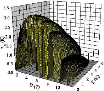
Figure 2:  Three dimensional phase diagrams in coordinates $T-H-T_{D}$ for beryllium. Above the surface $T_{D}=T_{D}(T,\mu_{0}H)$ the uniform phase exists, while below this surface the non-uniform phase (Condon domain structure) is formed.

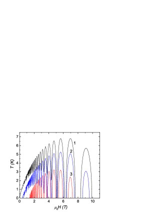
Figure 3:  Envelope of phase diagrams for beryllium $T-H$ (color online), estimated at three different Dingle temperatures: $T_{D}=0,1K$ and $2.1K$ (curves $1$) (black), $2$ (blue) and $3$ (red) correspondingly. The position of the maximums is not influenced by $T_{D}$, while the values of the maximums depend strongly on $T_{D}$, decreasing with increase of $T_{D}$.

Resent experimental results on observation of irreversible effects in beryllium Kramer2 , as well as giant parametric enhancement of non-linear effects Tsindlekht , allows us to verify the phase diagrams calculated in the framework of the assumptions (4). Undoubtedly, both of the observed effects, e.g. irreversibility Kramer2 and strong non-linear dynamics Tsindlekht are closely related to the electron instability at given temperature in increasing applied magnetic field. This instability results in the phase transition from uniform state to non-uniform one with formation of Condon domain structure. Both results Kramer2 -Tsindlekht indicate on the existence of the large scale periodicity of the measured effects relative to inverse magnetic field (see, Eq. (10)), which is additional one to the usual small scale periodicity of dHvA effect. Undoubtedly, the large scale periodicity of above-mentioned effects, measured at given temperature ($T=1.3K$ Kramer2 and $T=1.2K$ Tsindlekht ) is the result of the periodicity in the appearance of the non-uniform state and, therefore, can serve as an instrument for verification of the theoretical phase diagrams. Comparison between the theoretical phase diagrams calculated on the basis of the assumption 4 is illustrated by Fig. 4. In Fig. 4($a$) the calculated diamagnetic phase transition temperature is plotted as a function of applied magnetic field for Dingle temperature $T_{D}=2.2K$. In calculation of phase diagram we put $\beta=1.15$. In Fig. 4($b$) the amplitude of the third harmonic Kramer2 (in arbitrary units), arising in the conditions of electron instability, as a function of magnetic field is depicted. It is evident from the comparison the theoretical phase diagram and data Kramer2 , measured at $T=1.3K$, that non-linear response appears at the intervals of applied magnetic field, corresponding to the formation of the Condon domain structure. The inverse large scale period $\Delta F=28.7T$ 10 gives a good agreement between theory and experiment. Unfortunately, the relevant to our calculation measurements in Kramer2 were made only at fix temperature $T=1.3K$. The measurements of the temperature dependence of the non-linear response (together with the field dependencies) would make it possible to reconstruct the complete phase diagrams $T=T(\mu_{0}H)$ for beryllium.

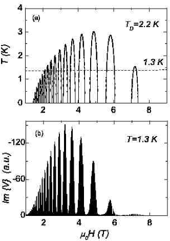
Figure 4:  Comparison computed phase diagrams with the data Kramer2 . Typical critical curve $T=T(\mu_{0}H)$ at given Dingle temperature $T_{D}=2.2K$ is shown ($a$). Figure ($b$) represents the experimental data Kramer2 on investigation of the irreversible effects in beryllium, which are the results of formation of Condon domain structure. The output signal is shown in arbitrary units. There is a good agreement between the intervals of existence of the non-uniform phase, estimated in the framework of (4), and the appearance of the observed in Kramer2 non-linear response.

IV Conclusions

We developed the model of slightly corrugated Fermi surface of beryllium with taking into account the negligible small curvature of the extreme cross sections of the Fermi surface sheet relevant to observation of dHvA oscillations. The calculated in the framework of our theory phase diagrams for beryllium are in a good agreement with available experimental data on observation of Condon domain instability.

The estimated phase diagrams reveal large scale periodicity on reciprocal magnetic field. The inverse period does not depends on the impurity of the sample and is related to the discrepancy of the two fundamental frequencies $\Delta F=28.7T$ Eq. (10) , corresponding to two extreme cross section of ’cigar’ like Fermi surface of beryllium, e.g. ’waist’ and ’hips’. The magnetic field dependencies of recent experimental data on observation of non-linear effects in beryllium Kramer2 -Tsindlekht have a simple explanation on the basis of the estimated diamagnetic phase diagrams. We hope that the theoretical results will stimulate further experiments on investigation of electron instability in strongly correlated electron systems. In particular, the measurements of the temperature dependencies of the non-linear effects in the samples of different impurity will allow constructing the complete phase diagrams.

- (1) D. Shoenberg, Magnetic Oscillations in Metals (Cambridge University Press, Cambridge, England, 1984).
- (2) J. H. Condon, Phys. Rev. 45, 526 (1966).
- (3) J. H. Condon and R. E. Walstedt, Phys. Rev. Lett. 21, 612 (1968).
- (4) R. G. Kramer, V. S. Egorov, V. A. Gasparov, A. G. M. Jansen, and W. Joss, Phys. Rev. Lett. 95, 267209 (2005).
- (5) G. Solt and V. S. Egorov, Physica B 318, 231 (2002).
- (6) R. G. Kramer, V. S. Egorov, A. G. M. Jansen, and W. Joss, Phys. Rev. Lett. 95, 187204 (2005).
- (7) M. I. Tsindlekht, N. Logoboy, V. S. Egorov, R. B. G. Kramer, A. G. M. Jansen, and W. Joss, Journal of Low Temp. Phys. (in press).
- (8) G. Solt, V. S. Egorov, C. Baines, D. Herlach, and U. Zimmermann, Physica B 326, 536 (2003).
- (9) G. Solt, Solid State Comm. 118, 231 (2001).
- (10) N. Logoboy, A. Gordon, I. D. Vagner, and W. Joss, Solid State Comm. 134, 497 (2005).
- (11) N. Logoboy, V. S. Egorov, and W. Joss, Solid State Comm. .
- (12) A. Gordon, N. Logoboy and W. Joss, Phys. Rev. B 137, 174417 (2006).
- (13) V. S. Egorov, Sov. Phys. Solid State 30, 1253 (1988).
- (14) J. Kübler, Theory of Itinerant Electron Magnetism, ( Clarendon Press, Oxford, England, 2000).
- (15) A. Gordon, I. Vagner, P. Wyder, Adv. in Phys. 52 385 (2003).