Spatially inhomogeneous states of charge carriers in graphene

Abstract

We study an interaction of 2D quasiparticles with linear dispersion $E=\pm u|p|$ (graphene) with impurity potentials. It is shown that in 1D potential well (quantum wire) there are discrete levels, corresponding to localized states, whereas in 2D well (quantum dot) there are no such states. Scattering cross-section of electrons (holes) of graphene by an axially symmetric potential well is found and it is shown that for infinetily large energy of incoming particles the cross-section tends to a constant. The effective Hamiltonian for a curved quantum wire of graphene is derived and it is shown that the corresponding geometric potential cannot form 1D bound states.

1 Introduction

Monatomic layer of carbon atoms, forming hexagonal lattice (graphene), is studied very intensively at present [1]-[3]. “Conical” dispersion law for quasiparticles (the name is borrowed from the similar 3D model of a gapless semiconductor) results in crucial distinctions of their dynamical characteristics from the corresponding characteristics of massive particles. The density of electron states tends linearly to zero as a function of energy $E$, counted from the conical point, that is more rapidly than for usual particles in 3D case ($\sqrt{E}$). This is a reason to expect that formation of bound states in potential wells will be hindered.

In the present paper we consider some simple exactly solvable models of 1D and 2D potential wells from the viewpoint of possibility to form bound states for quasiparticles , described by the Hamiltonian

$$\widehat{\mathcal{H}}=u\boldsymbol{\sigma\hat{p}},$$ (1)

where $\boldsymbol{\sigma}=(\sigma_{1},\sigma_{2})$ are Pauli matrices, $\boldsymbol{\hat{p}}=-i\hbar\nabla$ is momentum operator, $u$ is characteristic velocity (for graphene $u\sim 10^{6}$ m/sec). It turned out, that quantum wire (1D localization) is possible, whereas quantum dot as well as a hydrogen-like donor (acceptor) are not possible. 1D effective Hamiltonian for a curved wire will be derived and it will be shown that geometric potential differs significantly from the case of parabolic dispersion law.

Some problems of interaction of quasiparticles described by the Hamiltonian (1) with electrostatic potentials have recently been considered. In Ref. [4] the transmission coefficient of carriers through 1D barrier (p-n junction) is found; same authors have shown in Ref. [5] that Friedel oscillations of the charge density around an impurity atom in graphene differs essentially from the ones in 2D electron systems with parabolic dispersion law. Bound states in a symmetric 1D potential well have been investigated in Ref. [6]. We expound here solution of this problem (together with a more general one for an asymmetric well) as a starting point for our consideration of a curved quantum wire.

2 1D potential well

The motion of electrons in a graphene waveguide, representing 2D stripe with straight axis, is described by the equation:

$$u(\boldsymbol{\sigma\hat{p}})\Psi+v(y)\Psi=E\Psi,$$ (2)

where $v(y)$ is the potential confining the particle in the waveguide (below we suppose $u=\hbar=1$). Let us look for the solution in the form $\Psi(x,y)=\chi(y)\exp(ipx)$, where $\chi(y)=(\chi_{1},\chi_{2})$ is two-component spinor, whose components satisfy the equations:

$$\left(-\frac{\partial}{\partial y}+p\right)\chi_{2}=(E-v(y))\chi_{1}\quad\left(\frac{\partial}{\partial y}+p\right)\chi_{1}=(E-v(y))\chi_{2}.$$ (3)

After excluding $\chi_{2}$, we find:

$$\left[-\frac{\partial^{2}}{\partial y^{2}}+p^{2}+\left(\frac{\partial}{\partial y}\ln(E-v(y))\right)\left(\frac{\partial}{\partial y}+p\right)\right]\chi_{1}=\left(E-v(y)\right)^{2}\chi_{1}$$ (4)

Substituting $\chi_{1}$ in the form $\sqrt{E-v(y)}\widetilde{\chi}_{1}$, we obtain

$$\left[-\frac{\partial^{2}}{\partial y^{2}}+p^{2}-(E-v(y))^{2}+\frac{v^{\prime\prime}(y)/2-v^{\prime}(y)p}{E-v(y)}+\frac{3(v^{\prime}(y))^{2}}{4(E-v(y))^{2}}\right]\widetilde{\chi}_{1}=0$$ (5)

The equation for function $\chi_{2}=\sqrt{E-v(y)}\widetilde{\chi}_{2}$ is obtained by means of replacement $p\rightarrow-p$.

Let us consider the potential $v(y)$ in the form of step function: $v(y)=0$ if $y<-a$, $v(y)=-v_{0}$ if $|y|<a$, $v(y)=-v_{1}$ if $y>a$. In each region the equation (5) is reduced to

$$-\partial^{2}\chi_{1}/\partial y^{2}=[(E-v_{i})^{2}-p^{2}]\chi_{1},$$

where $v_{i}=0$ if $y<-a$, $v_{i}=-v_{0,1}$ if $|y|<a$ and $y>a$ correspondingly. Solutions of the last equation decreasing when $y\to\pm\infty$, have the form $\chi_{1}=A_{1}e^{\varkappa y}$ if $y<-a$, $\chi_{1}=B_{1}\sin qy+B_{2}\cos qy$ if $|y|<a$, $\chi_{1}=A_{3}e^{-\varkappa_{1}y}$ if $y>a$. Here $\varkappa=\sqrt{p^{2}-E^{2}}$, $q=\sqrt{(E+v_{0})^{2}-p^{2}}$, $\varkappa_{1}=\sqrt{p^{2}-(E+v_{1})^{2}}$.

Matching conditions $\chi_{i}|_{y=\pm a-0}=\chi_{i}|_{y=\pm a+0}$, $i=1,2$ lead to the following equation, determining the spectrum $E=E^{\nu}(p)$, where $\nu$ is the number of subband of transversal quantization:

$$\left[1-\frac{\varkappa+p}{E}\ \frac{\varkappa_{1}-p}{E+v_{1}}+\frac{p}{E+v_{0}}\ \frac{\varkappa_{1}-p}{E+v_{1}}-\frac{\varkappa+p}{E}\frac{p}{E+v_{0}}\right]\sin(2qa)-$$

$$-\frac{q}{E+v_{0}}\left[\frac{\varkappa_{1}-p}{E+v_{1}}+\frac{\varkappa+p}{E}\right]\cos(2qa)=0.$$ (6)

In the case of symmetric well $v_{1}=0,\,\varkappa_{1}=\varkappa$; equation (6) is simplified:

$$[E(E+v_{0})-p^{2}]\sin(2qa)-\varkappa q\cos(2qa)=0.$$ (7)

Branches $E^{\nu}(p)$ for symmetric well are shown on Fig.1. Let us note that equation (7) always has the solution $E(p)=|p|-v_{0}$, i.e. $q=0$. However this branch of the spectrum is not physical since it corresponds to the wavefunction identically equaled to zero.

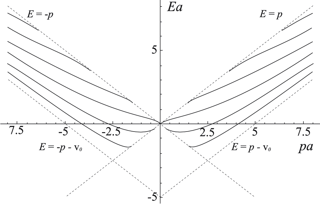
Figure 1: Bound states $E(p)$ in the 1D symmetric rectangular well; $v_{0}a=5$. Dotted line shows the bounds of the area, occupied by discrete spectrum.

Investigation of the equation (7) leads to the condition of reality of $q$, which, together with obvious condition of reality of $\varkappa$, determines the region, occupied by discrete spectrum $\max\{-|p|,|p|-v_{0}\}<E<|p|$. From this, in particular, it follows that $E>-v_{0}/2$. It is easy to calculate energy in the following limiting cases:

$$1) |p|\ll v_{0},\cos(2v_{0}a)\neq 0: E(p)=|p|{\rm sign}\{\sin(2v_{0}a)\}\cos(2v_{0}a),$$ (8)

$$2) |p|\ll v_{0},\cos(2v_{0}a)=0: E(p)=p^{2}/v_{0},$$ (9)

$$3) v_{0}\to 0\ \ \textrm{ }\ \ a\to 0: E=|p|(1-2v_{0}^{2}a^{2}+\ldots).$$ (10)

In the shallow asymmetric well there are no bound states at any $p$. There are no bound states also in an asymmetric well of any depth at small enough $p$.

3 Effective 1D equation in adiabatically curved stripe

Let us consider a stripe with curved axis defined by the equation $\boldsymbol{r}=\boldsymbol{R}(x);$ we suppose the stripe to be curved in its plane. Here $\boldsymbol{R}(x)=(R_{1}(x),R_{2}(x))$ is a smooth vector-function, $x$ is the natural parameter on the axis (length counted out from some fixed point), $|d\boldsymbol{R}/dx|=1$. Let $\boldsymbol{n}(x)=\bigl{(}n_{1}(x),n_{2}(x)\bigr{)}$ be the unitary vector normal to $d\boldsymbol{R}/dx$. In the neighborhood of axis the curvilinear coordinates $x,\,y$, defined by the equality $\boldsymbol{r}=\boldsymbol{R}(x)+y\boldsymbol{n}(x)$ can be introduced. The equation (2) in curvilinear coordinates has the form:

$$\left[\frac{(\boldsymbol{\sigma R}^{\prime})}{\sqrt{1-ky}}(-i\frac{\partial}{\partial x})\frac{1}{\sqrt{1-ky}}+(\boldsymbol{\sigma n})(-i\frac{\partial}{\partial y})-\frac{ik(\boldsymbol{\sigma n})}{2(1-ky)}+v(y)\right]\widetilde{\Psi}=E\widetilde{\Psi},$$ (11)

where $k$ is the curvature of the axis of waveguide at the point $x$, $\widetilde{\Psi}=(1-ky)^{1/2}\Psi$. Let us take into account now that the stripe is curved adiabatically, i.e. formally $k\to 0$. Following the idea [7], we look for the solution of the last equation in the form $\Psi^{\nu}(x,y)=\hat{\chi}^{\nu}\psi^{\nu}(x)$, $\hat{\chi}^{\nu}=(\hat{\chi}^{\nu}_{1},\hat{\chi}^{\nu}_{2})$ is two-component vector-operator and scalar wavefunction $\psi^{\nu}(x)$ satisfies effective Schrödinger equation

$$\hat{L}^{\nu}\psi^{\nu}(x)=E\psi^{\nu}(x).$$ (12)

Now we expand the operator $\hat{L}$ in powers of curvature $\hat{L}^{\nu}=\hat{H}_{\rm eff}^{\nu}+\hat{L}_{1}^{\nu}+\ldots$. It will be shown that operator $\hat{H}_{\rm eff}^{\nu}=H_{\rm eff}^{\nu}(-i\partial/\partial x)$ does not depend on $x$. It follows from [8] that $H_{\rm eff}^{\nu}(p)$ is an eigenvalue of the following problem:

$$\left[(\boldsymbol{\sigma R}^{\prime})p+(\boldsymbol{\sigma n})(-i\frac{\partial}{\partial y})+v(y)\right]\chi^{\nu}(p,x,y)=H_{\rm eff}^{\nu}(p)\chi^{\nu}(p,x,y),$$ (13)

where $p$ is a parameter ($c$-number), $\chi^{\nu}=(\chi_{1}^{\nu},\chi_{2}^{\nu})$. Using the replacement $\chi_{2}^{\nu}=(n_{2}-in_{1})\widetilde{\chi}_{2}^{\nu}$ we reduce (13) to (3):

$$\left[p-\frac{\partial}{\partial y}\right]\widetilde{\chi}_{2}^{\nu}=\bigl{(}H_{\rm eff}^{\nu}(p)-v(y)\bigr{)}\chi_{1}^{\nu},\quad\left[p+\frac{\partial}{\partial y}\right]\chi_{1}^{\nu}=\bigl{(}H_{\rm eff}^{\nu}(p)-v(y)\bigr{)}\widetilde{\chi}_{2}^{\nu}.$$ (14)

It follows from the last equation that $H_{\rm eff}^{\nu}(p)=E^{\nu}(p)$, i.e. $H_{\rm eff}^{\nu}$ does not depend on $x$. Let us choose functions $\chi_{1}^{\nu},\,\widetilde{\chi}_{2}^{\nu}$ to be real. Then from general formulae [8] and the relation $\left\langle(\chi^{\nu})^{+}(\boldsymbol{\sigma n})\chi^{\nu}\right>_{y}=0$ it follows that

$$\hat{L}_{1}^{\nu}=\left[k(x),\bigl{(}2K(\hat{p})\hat{p}+Q(\hat{p})\bigr{)}\right]_{+},\quad K(p)=\left\langle\chi_{1}^{\nu}y\widetilde{\chi}_{2}^{\nu}\right>_{y},\quad Q(p)=\left\langle\chi_{1}^{\nu}\widetilde{\chi}_{2}^{\nu}\right>_{y}.$$ (15)

Here $\hat{p}=-i\partial/\partial x$, $[\cdot,\cdot]_{+}$ means anticommutator, and $\left<\cdot\right>_{y}$ means integration over $y$. For even potential $K(p)=0$.

Effective equation for rectangular well at small $|p|$. For symmetric rectangular well at small $|p|$ one can use dispersion relation (8). Then we find $Q(0)={\rm sign}\{\sin(2v_{0}a)\}{\rm sign}\{\hat{p}\}\cos(2v_{0}a)/2$. Effective 1D equation for small momentums takes the form:

$${\rm sign}\{\sin(2v_{0}a)\}{\rm sign}\{\hat{p}\}\left(-i\frac{\partial}{\partial x}+\frac{k(x)}{2}\right)\psi=E\psi$$ (16)

Thus, the geometric potential for quasiparticles has the form $k(x)/2$ and, how one can see from (16), it cannotform bound states.

4 Axially symmetric potential

Let us consider the equation (2) for the axially-symmetric potential. In the cylindric coordinates $x=r\cos\varphi,\,y=r\sin\varphi$ it has the form

$$e^{-i\varphi}\left(-i\frac{\partial}{\partial r}-\frac{1}{r}\frac{\partial}{\partial\varphi}\right)\Psi_{2}=(E-v(r))\Psi_{1},\quad e^{i\varphi}\left(-i\frac{\partial}{\partial r}+\frac{1}{r}\frac{\partial}{\partial\varphi}\right)\Psi_{1}=(E-v(r))\Psi_{2}.$$ (17)

We find the solution in the form $\Psi_{1}=e^{in\varphi}\chi_{1},\,\Psi_{2}=e^{i(n+1)\varphi}\chi_{2}$, where $\chi_{1},\,\chi_{2}$ satisfy equations

$$\left(-i\frac{\partial}{\partial r}-\frac{i(n+1)}{r}\right)\chi_{2}=(E-v(r))\chi_{1},\quad\left(-i\frac{\partial}{\partial r}+\frac{in}{r}\right)\chi_{1}=(E-v(r))\chi_{2}.$$ (18)

4.1 Rectangular well

Let us consider axially symmetric well with constant width: $v(r)=-v_{0}$ if $r<a$ and $v(r)=0$ if $r\geq a$. Excluding $\chi_{2}$ from (18), we obtain:

$$\left\{-\frac{\partial^{2}}{\partial r^{2}}-\frac{1}{r}\frac{\partial}{\partial r}+\frac{n^{2}}{r^{2}}-(E+v_{0})^{2}\right\}\chi_{1}=0,\quad r<a,$$ (19)

$$\left\{-\frac{\partial^{2}}{\partial r^{2}}-\frac{1}{r}\frac{\partial}{\partial r}+\frac{n^{2}}{r^{2}}-E^{2}\right\}\chi_{1}=0,\quad r\geq a.$$ (20)

These equations have solutions $J_{n}(|E+v_{0}|r),\,N_{n}(|E+v_{0}|r)$ and $J_{n}(|E|r),\,N_{n}(|E|r)$ correspondingly. The solution regular in the point $r=0$ has the form $\chi_{1}(r<a)=C_{n}J_{n}((E+v_{0})r)$.

The equation (20) contains only the square of the energy. Thus its solutions don’t depend on the sign of $E$. These solutions are equivalent to scattering states of the usual radial Schrödinger equation with $E>0$. From this circumstance one can conclude that there are no bound states in such a potential well. We would like to emphasize that this conclusion does not depend on the depth and width of the well, i.e. 2D localization of quasiparticals in graphene (quantum dot) is principally impossible (naturally, this statement only relates to the region of momenta where the Hamiltonian (2) and linear dispersion law are valid). The same is true, obviously, for any potential decreasing at the infinity, hence, hydrogen-like states of donors or acceptors in graphene do not exist.

Let us consider now the scattering problem. Let the wave with positive energy comes from the infinity along the $x$-axis. Then the wavefunction $\Psi$ far from the origin has the form:

$$\Psi\simeq\frac{e^{i|E|r\cos\varphi}}{\sqrt{2}}\begin{pmatrix}1\\ 1\end{pmatrix}+\frac{e^{i|E|r}}{\sqrt{r}}\begin{pmatrix}f_{1}(\varphi)\\ f_{2}(\varphi)\end{pmatrix}.$$ (21)

Using the expansion of the plane wave $\exp(i|E|r\cos\varphi)=({1}/{2})\sum_{n=-\infty}^{\infty}i^{n}[H_{n}^{(1)}(|E|r)+H_{n}^{(2)}(|E|r)]\exp(in\varphi),$ we can represent the solution in the form

$$\Psi=\frac{1}{2}\sum_{n=-\infty}^{\infty}\begin{pmatrix}i^{n}e^{in\varphi}(S_{n}^{(1)}H_{n}^{(1)}(|E|r)+2^{-1/2}H_{n}^{(2)}(|E|r))\\ i^{n}e^{in\varphi}(S_{n}^{(2)}H_{n}^{(1)}(|E|r)+2^{-1/2}H_{n}^{(2)}(|E|r))\end{pmatrix}.$$ (22)

Hence

$$f_{1}(\varphi)=\frac{e^{-i\pi/4}}{\sqrt{2\pi|E|}}\sum_{n=-\infty}^{\infty}e^{in\varphi}(S_{n}^{(1)}-2^{-1/2}),$$

$$f_{2}(\varphi)=\frac{e^{-i\pi/4}}{\sqrt{2\pi|E|}}\sum_{n=-\infty}^{\infty}e^{in\varphi}(S_{n}^{(2)}-2^{-1/2})$$ (23)

Withfunctional relations for Hankel functions, it is easy to show that $S_{n+1}^{(2)}=S_{n}^{(1)}$. Hence $f_{2}(\varphi)=e^{i\varphi}f_{1}(\varphi).$ Continuity conditions for the wavefunction at $r=a$ lead to the equations:

$$S_{n}^{(1)}H_{n}^{(1)}(|E|a)+2^{-1/2}H_{n}^{(2)}(|E|a)=C_{n}J_{n}(|E+v_{0}|a),$$ (24)

$$S_{n}^{(1)}H_{n+1}^{(1)}(|E|a)+2^{-1/2}H_{n+1}^{(2)}(|E|a)=C_{n}J_{n+1}(|E+v_{0}|a)$$ (25)

From these equations one can find $S_{n}^{(1)}$, $S_{n}^{(2)}$. Wavefunction of the scattered particles has the form $\Psi_{out}\simeq{e^{i|E|r}}r^{-1/2}(f_{1}(\varphi),f_{2}(\varphi)),$ and the current density is given by $\boldsymbol{j}_{out}=\Psi_{out}^{+}\boldsymbol{\sigma}\Psi_{out}={2|f_{1}(\varphi)|^{2}}r^{-1}\{\cos\varphi,\sin\varphi\}$ (we write Cartesian components of the current in braces). Thus, the differential cross-section is ${d\sigma}/{d\varphi}=2\,|f_{1}(\varphi)|^{2}.$ Total cross-section is

$$\sigma=2\int_{0}^{2\pi}|f_{1}(\varphi)|^{2}d\varphi=\frac{1}{|E|}\sum_{n=-\infty}^{\infty}|S_{n}+1|^{2}=$$

$$=\frac{8}{|E|}\sum_{n=0}^{\infty}\left|\frac{J_{n}(|E+v_{0}|a)J_{n+1}(|E|a)-J_{n+1}(|E+v_{0}|a)J_{n}(|E|a)}{J_{n}(|E+v_{0}|a)H_{n+1}^{(1)}(|E|a)-J_{n+1}(|E+v_{0}|a)H_{n}^{(1)}(|E|a)}\right|^{2}.$$ (26)

Similar calculations lead to the same formula for the total cross-section for particles with negative energy. In the low-energy limit $|E|a\ll 1$ the asymptotic formulae $J_{0}(z)=1+O(z^{2}),\,J_{1}(z)=z/2+O(z^{2}),\,N_{0}(z)={\rm const}+2\ln(z)/\pi+O(z),\,N_{1}(z)=-2/(\pi z)+O(z^{0})$ result in

$$\sigma\simeq 2\left(\frac{\pi J_{1}(v_{0}a)}{J_{0}(v_{0}a)}\right)^{2}|E|a^{2}$$ (27)

In Fig.2 we show the scattering cross-section as a function of $|E|a$. One can see that cross-section has resonances. We will study below the opposite limiting case $|E|a\gg 1$ for which a different method is more convenient.

Figure 2: Scattering cross-section by rectangular axially symmetric well with radius $a$, $v_{0}a=\pi$.

4.2 Green function and integral equation for the scattering problem

Green function of the operator (1) is $2\times 2$-matrix $G(\boldsymbol{r})$. It satisfies the equation

$$[(\boldsymbol{\sigma\hat{p}})-E]G(\boldsymbol{r};E)=\delta(\boldsymbol{r})I,\qquad G=\begin{pmatrix}g_{11}&&g_{12}\\ g_{21}&&g_{22}\end{pmatrix},\qquad I=\begin{pmatrix}1&&0\\ 0&&1\end{pmatrix}.$$ (28)

Solving this equation we find

$$G(\boldsymbol{r};E)=\frac{1}{4}\begin{pmatrix}iEH_{0}^{(1)}(|E|r)&&|E|e^{-i\varphi}\bigl{(}H_{0}^{(1)}\bigr{)}^{\prime}(|E|r)\\ |E|e^{i\varphi}\bigl{(}H_{0}^{(1)}\bigr{)}^{\prime}(|E|r)&&iEH_{0}^{(1)}(|E|r)\end{pmatrix}.$$ (29)

For large $|E|r$ Green function has the asymptotic form

$$G(\boldsymbol{r};E)\simeq\sqrt{\frac{|E|}{8\pi r}}e^{i\left(|E|r+{\pi}/{4}\right)}\begin{pmatrix}{\rm sign}(E)&&e^{-i\varphi}\\ e^{i\varphi}&&{\rm sign}(E)\end{pmatrix}.$$ (30)

The scattering is described by the integral equation

$$\Psi(\boldsymbol{r};E)=\Psi_{in}(\boldsymbol{r};E)-\int G(\boldsymbol{r}-\boldsymbol{r^{\prime}};E)v(\boldsymbol{r^{\prime}})\Psi(\boldsymbol{r^{\prime}};E)d^{2}\boldsymbol{r^{\prime}},$$ (31)

where $\Psi_{in}$ is the wavefunction of incoming particles. In the first Born approximation we obtain:

$$\Psi(\boldsymbol{r};E)=\Psi_{in}(\boldsymbol{r};E)-\frac{v_{0}a}{2q}\sqrt{\frac{\pi|E|}{r}}e^{i\left(|E|r+{\pi}/{4}\right)}\begin{pmatrix}1+e^{-i\varphi}\\ {\rm sign}(E)\,(1+e^{i\varphi})\end{pmatrix}J_{1}(qa),$$ (32)

where $q=2|E|\sin(\varphi/2)$. Scattering cross-section is

$$\frac{d\sigma}{d\varphi}=\frac{2\pi|E|v_{0}^{2}a^{2}}{q^{2}}\cos^{2}(\varphi/2)J_{1}^{2}(qa)=\frac{\pi v_{0}^{2}a^{2}}{2|E|}\cot^{2}(\varphi/2)J_{1}^{2}\bigl{(}2|E|a\sin(\varphi/2)\bigr{)},$$

$$\sigma=\frac{\pi^{2}v_{0}^{2}a^{4}|E|}{2}\ {}_{2}F_{3}[1/2,3/2;2,2,3;-4|E|^{2}a^{2}],$$ (33)

where ${}_{2}F_{3}$ is the generalized hypergeometric function.

When $|E|a\to\infty$ scattering cross-section tends to the constant $\sigma\to{16v_{0}^{2}a^{3}}/{3}$. Note that for usual particles the Born scattering cross-section by a short-range potential tends to zero when energy increases [9], however if one formally supposes the mass to be proportional to momentum (to obtain the linear dispersion law), then limiting value of the Born cross-section at $|E|\to\infty$ also turns out to be constant.

Acknowledgements:- The authors would like to thank M. V. Entin and V. M. Kovalev for useful discussions. This work has been supported by THE RFBR (grant no. 05-02-16939), The Council of The President of The RF for scientific schools (gr. 4500, 2006.2) and by the programs of The Russian Academy of Sciences.

References

• [1] K. S. Novoselov et al., Science, 306, 666 (2004).
• [2] Y. Zhang et al., Nature, 438, 201 (2005).
• [3] K. S. Novoselov, A. K. Geim, S. V. Morozov, D. Jiang, M. I. Katsnelson, I. V. Grigorieva, S. V. Dubonos, A. A. Firsov, Nature, 438, 197 (2005).
• [4] V. V. Cheianov and V. I. Fal ko, Phys. Rev. B 74, 041403(R) (2006).
• [5] V. V. Cheianov and V. I. Fal ko, arXiv:cond-mat/0608228 v1 10 Aug 2006.
• [6] J. Milton Pereira, Jr., V. Mlinar, F. M. Peeters, P. Vasilopoulos, Phys. Rev. B 74, 045424 (2006).
• [7] L. V. Berlyand and S. Yu. Dobrokhotov, Sov. Phys. Doklady, 32, (1987), 714 -716.
• [8] V. V. Belov, S. Yu. Dobrokhotov, T. Ya. Tudorovskiy, J. Eng. Math., 55, 1, (2006), 179–233.
• [9] L. D. Landau and E. M. Lifshitz, Quantum Mechanics: (Nonrelativistic Theory). In: Theoretical Physics 3, Oxford, London, Edinburgh: Pergamon Press (1965) ix+616pp.