Coherent dynamics on hierarchical systems

Abstract

We study the coherent transport modeled by continuous-time quantum walks, focussing on hierarchical structures. For these we use Husimi cacti, lattices dual to the dendrimers. We find that the transport depends strongly on the initial site of the excitation. For systems of sizes $N\leq 21$, we find that processes which start at central sites are nearly recurrent. Furthermore, we compare the classical limiting probability distribution to the long time average of the quantum mechanical transition probability which shows characteristic patterns. We succeed in finding a good lower bound for the (space) average of the quantum mechanical probability to be still or again at the initial site.

Introduction
The dynamics of excitons is a problem of long standing in molecular and polymer physics Kenkre . Thus, the incoherent exciton transport can be efficiently modeled by random walks, see, for instance, heijs2004 ; blumen2005 ; then, the transport follows a master (rate) equation and the underlying topology is fundamental for the dynamics weiss . Studying the coherent transport, we model the process using Schrödinger’s equation, which is mathematically closely related to the master equation, where the transfer rates enter through the connectivity matrix ${\bf A}$ of the structure farhi1998 ; mb2005a ; mvb2005a . Moreover, also the elements of the secular matrix in Hückel’s theory are given by ${\bf A}$ McQuarrie .

Hyperbranched macromolecules have attracted a lot of attention in recent years. In this respect dendrimers have served as a prime example Voegtle . Among a series of very interesting and crossdisciplinary applications like drug delivery, the role of dendrimers as light harvesting antennae has been investigated mukamel1997 ; jiang1997 ; barhaim1997 ; barhaim1998 . The details of the transport of an optical excitation over these structures depend on the localized states used. In one picture one may envisage the excitation to occupy the branching points of the dendrimer, see, for instance, barhaim1997 ; barhaim1998 ; mbb2006a . However, as shown in poliakov1999 , it may happen that the exciton occupies preferentially the bonds between the branching points. Then, the essential underlying structure is different and is given by sites localized at the mid-points of the bonds. We exemplify the situation in Fig. 1(a), starting from a dendrimer of generation $2$ (open circles) and indicating the mid-points of the bonds by filled circles. Connecting neighboring filled circles by new bonds, one is led to the dual lattice of the dendrimer, which is called a Husimi cactus. Figure 1 shows three finite Husimi cacti of sizes $N=9,21$, and $45$.

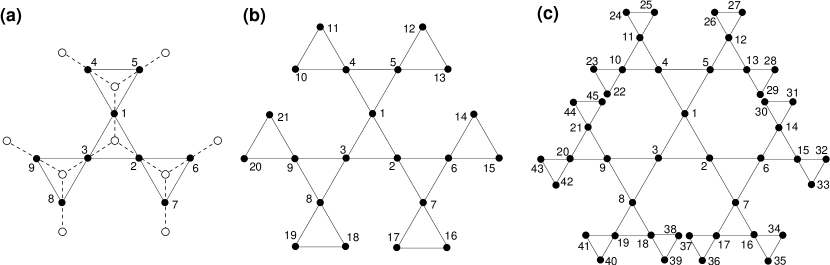
Figure 1: Finite Husimi cacti (filled circles) of size (a) $N=9$, (b) $N=21$, and (c) $N=45$. (a) also shows with dashed lines and open circles the corresponding dendrimer.

Coherent dynamics modelled by quantum walks
The quantum mechanical extension of a continuous-time random walk (CTRW) on a network (graph) of connected nodes is called a continuous-time quantum walk (CTQW). It is obtained by identifying the Hamiltonian of the system with the (classical) transfer matrix, ${\bf H}=-{\bf T}$, see e.g. farhi1998 ; mb2005a (we will set $\hbar\equiv 1$ and $m\equiv 1$ in the following). The transfer matrix of the walk, ${\bf T}=(T_{ij})$, is related to the connectivity matrix ${\bf A}$ of the graph by ${\bf T}=-\gamma{\bf A}$, where for simplicity we assume the transmission rates $\gamma$ of all bonds to be equal and set $\gamma\equiv 1$ in the following. The matrix ${\bf A}$ has as non-diagonal elements $A_{ij}$ the values $-1$ if nodes $i$ and $j$ of the graph are connected by a bond and $0$ otherwise. The diagonal elements $A_{ii}$ of ${\bf A}$ equal the number of bonds, $f_{i}$, which exit from node $i$.

The basis vectors $|j\rangle$ associated with the nodes $j$ span the whole accessible Hilbert space to be considered here. The time evolution of a state $|j\rangle$ starting at time $t_{0}$ is given by $|j;t\rangle={\bf U}(t,t_{0})|j\rangle$, where ${\bf U}(t,t_{0})=\exp[-i{\bf H}(t-t_{0})]$ is the quantum mechanical time evolution operator. The transition amplitude $\alpha_{k,j}(t)$ from state $|j\rangle$ at time $0$ to state $|k\rangle$ at time $t$ reads then $\alpha_{k,j}(t)=\langle k|{\bf U}(t,0)|j\rangle$ and obeys Schrödinger’s equation. Denoting the orthonormalized eigenstates of the Hamiltonian ${\bf H}=-{\bf T}$ by $|q_{n}\rangle$ (such that $\sum_{n}|q_{n}\rangle\langle q_{n}|=\boldsymbol{1}$) and the corresponding eigenvalues by $\lambda_{n}$, the quantum mechanical transition probability (TP) is

$$\pi_{k,j}(t)\equiv|\alpha_{k,j}(t)|^{2}=\left|\sum_{n}\langle k|e^{-i\lambda_{n}t}|q_{n}\rangle\langle q_{n}|j\rangle\right|^{2}.$$ (1)

Note that for the corresponding classical probabilities $\sum_{k}p_{k,j}(t)=1$ holds, with $p_{k,j}(t)=\sum_{n}\langle k|e^{-\lambda_{n}t}|q_{n}\rangle\langle q_{n}|j\rangle$, whereas quantum mechanically we have $\sum_{k}|\alpha_{k,j}(t)|^{2}=1$.

Transition probabilities
In the following we present the TPs $\pi_{k,j}(t)$ obtained from diagonalizing the Hamiltonian ${\bf H}$ by using the standard software package MATLAB. For the finite Husimi cactus consisting of $21$ nodes, as depicted in Fig. 1, we find numerically that the TPs are nearly periodic when the initial excitation is placed on one of the (symmetrically equivalent) nodes $1$, $2$, or $3$ of the inner triangle. Thus at time $t=35.551846$ one has $\pi_{1,1}(35.551846)=0.998761$, when starting from $\pi_{1,1}(0)=1$. In fact, the following expression holds exactly for all $k$ sites of the cactus with $N=21$:

$$\pi_{k,1}(t)=\left[\sum_{l=1}^{6}a_{l}^{(k)}\cos(\lambda_{l}t)\right]^{2}+\left[\sum_{l=1}^{6}a_{l}^{(k)}\sin(\lambda_{l}t)\right]^{2}.$$ (2)

Here $\lambda_{1}=0$, $\lambda_{2}=3$, $\lambda_{3}=3+\sqrt{2}$, $\lambda_{4}=3-\sqrt{2}$, $\lambda_{5}=3+2\sqrt{2}$, $\lambda_{6}=3-2\sqrt{2}$, and the $a_{l}^{(k)}$ follow from the corresponding eigenvectors. We further remark that the $N=21$ cactus has $8$ distinct eigenvalues, but that not all of them enter $\pi_{k,1}(t)$.

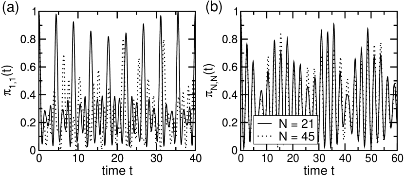
Figure 2: Transition probabilities $\pi_{j,j}(t)$ of the transport over finite Husimi cacti of sizes $N=21$ (full lines) and $N=45$ (dashed lines) for (a) $j=1$ and (b) $j=N$.

Figure 2 shows the probability to be at the initial node after time $t$ for two different sizes $N$ and two different initial conditions. For $N=21$, when the excitation starts at the core ($j=1$), the TP $\pi_{1,1}(t)$ is nearly recurrent. This is not anymore the case for $N=45$. Moreover, when the excitation starts at the periphery ($j=N$), the TPs $\pi_{N,N}(t)$ are even more irregular. Now the $\pi_{k,N}(t)$ for $N=21$ with $j=N$ indeed also contain the two eigenvalues $\lambda_{7}=3+\sqrt{6}$ and $\lambda_{8}=3-\sqrt{6}$ in addition to those given after Eq. (2), a fact which increases the irregularity of the temporal behavior of the $\pi_{k,N}(t)$.

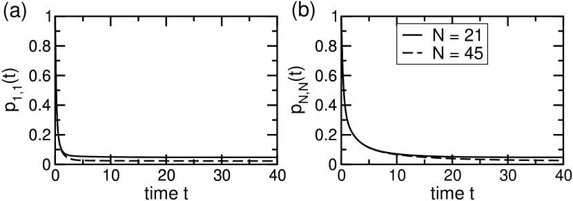
Figure 3: Classical transition probabilities $p_{j,j}(t)$ of the transport over finite Husimi cacti of sizes $N=21$ (full lines) and $N=45$ (dashed lines) for (a) $j=1$ and (b) $j=N$.

For comparison we also show in Fig. 3 the classical transition probabilities $p_{j,j}(t)$ for the same initial conditions as in the previous CTQW. Also here, there is a difference between the starting points. If the excitation starts at the central node $1$, the equipartitioned limiting probability $1/N$ is reached much faster than when starting at the periphery.

Long time limit
The quantum mechanical time evolution is symmetric to inversion. This prevents $\pi_{k,j}(t)$ from having a definite limit for $t\to\infty$. In order to compare the classical long time probability with the quantum mechanical one, one usually uses the limiting probability (LP) distribution aharonov2001

$$\chi_{k,j}\equiv\lim_{T\to\infty}\frac{1}{T}\int_{0}^{T}dt\ \pi_{k,j}(t),$$ (3)

which can be rewritten by using the orthonormalized eigenstates of the Hamiltonian, $|q_{n}\rangle$, as mvb2005a ; mbb2006a

$$\chi_{k,j}=\sum_{n,m}\delta_{\lambda_{n},\lambda_{m}}\langle k|q_{n}\rangle\langle q_{n}|j\rangle\langle j|q_{m}\rangle\langle q_{m}|k\rangle.$$ (4)

Some eigenvalues of $\bf H$ might be degenerate, so that the sum in Eq. (4) can contain terms belonging to different eigenstates $|q_{n}\rangle$ and $|q_{m}\rangle$.

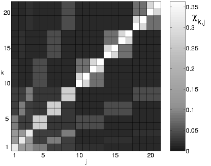
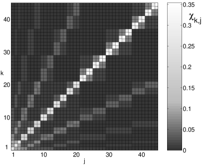
Figure 4: Limiting probabilites for finite Husimi cacti of sizes $N=21$ (left) and $N=45$ (right).

In Fig. 4 we present the LPs for two sizes of Husimi cacti, $N=21$ and $N=45$. The LP distributions are self-similar generation after generation. Furthermore, for each size there are LPs having the same value, i.e. $\chi_{k,j}=\chi_{l,j}$. We collect LPs of the same value into clusters. Depending on where the excitation starts, the clustering is different. For instance, for $N=21$, with an excitation starting at node $1$, there are $6$ different clusters, namely node $1$ forms one cluster and the nodes $\{2,3\}$, $\{4,5\}$, $\{6,7,8,9\}$, $\{10,11,12,13\}$, and $\{14,\cdots,21\}$ the remaining $5$ clusters. When the excitation starts at another node, the clusters are formed by different nodes, as can be infered from Fig. 4.

These results are closely related to our findings for the coherent transport over dendrimers mbb2006a . For dendrimers the grouping of sites into clusters also depends on the starting site. Furthermore, there exists a lower bound for the LPs; one has namely $\chi_{k,j}\geq 1/N^{2}$ for all nodes $k$ and $j$ mbb2006a . This lower bound is related to the fact that in our cases ${\bf A}$ has exactly one vanishing eigenvalue, $\lambda_{0}=0$.

Averaged probabilities
As discussed above, starting at a central node of the $N=21$ cactus, say node $1$, leads to nearly periodic $\pi_{k,1}(t)$. However, for larger cacti and/or different initial conditions this does not have to be the case.

Classically one has a very simple expression for the probability to be still or again at the initially excited node, spacially averaged over all nodes. Then one finds blumen2005

$$\overline{p}(t)\equiv\frac{1}{N}\sum_{j=1}^{N}p_{j,j}(t)=\frac{1}{N}\sum_{n=1}^{N}\ \exp\big{(}-\lambda_{n}t\big{)}.$$ (5)

This result is quite remarkable, since it depends only on the eigenvalue spectrum of the connectivity matrix, but not on the eigenvectors.

Quantum mechanically, we obtain a lower bound by using the Cauchy-Schwarz inequality, i.e., mbb2006a ,

$$\overline{\pi}(t)\equiv\frac{1}{N}\sum_{j=1}^{N}\pi_{j,j}(t)\geq\frac{1}{N^{2}}\sum_{n,m}\ \exp\big{[}-i(\lambda_{n}-\lambda_{m})t\big{]}.$$ (6)

In analogy to the classical case, the lower bound in Eq. (6) depends only on the eigenvalues and not on the eigenvectors. Note that for a CTQW on a simple regular network with periodic boundary conditions the lower bound is exact. We sketch the proof for a $1$D regular network of length $N$. There, the transition amplitudes to be still or again at node $j$ after time $t$ read $\alpha_{j,j}(t)=N^{-1}\sum_{n}\exp(-i\lambda_{n}t)$, see Eq. (16) of mb2005b with $\lambda_{n}=2-2\cos(2\pi n/N)$. The average $\overline{\pi}(t)$ is then given by

$$\overline{\pi}(t)=\frac{1}{N}\sum_{j=1}^{N}\left|\frac{1}{N}\sum_{n}\exp(-i\lambda_{n}t)\right|^{2}=\frac{1}{N^{2}}\sum_{n,m}\ \exp\big{[}-i(\lambda_{n}-\lambda_{m})t\big{]}.$$ (7)

This result also holds for hypercubic lattices in higher, $d$-dimensional spaces, when the problem separates in every direction; then one has $\alpha^{(d)}_{j,j}(t)=[\alpha_{j,j}(t)]^{d}$ (for the $d=2$ case see mvb2005a ).

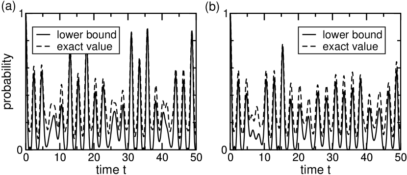
Figure 5: Comparison of the averaged probability to be still or again at the initial node with the lower bound given in Eq. (6) for finite Husimi cacti of sizes (a) $N=21$ and (b) $N=45$.

In Fig. 5 we compare the exact value of $\overline{\pi}(t)$ with the lower bound given in Eq. (6). We use cacti of two different sizes, namely $N=21$ and $N=45$. Now, the lower bound fluctuates more than the exact curve, but it reproduces quite well the overall behavior of the extrema of the exact curve. Especially the strong maxima of the exact value are quantitatively reproduced. This is in accordance with previous studies on exciton transport over square lattices mvb2005a and over dendrimers mbb2006a .

Conclusions
In conclusion, we have modeled the coherent dynamics on finite Husimi cacti by continuous-time quantum walks. The transport is only determined by the topology, i.e. by the connectivity matrix, of the cacti. For the $N=21$ cactus the dynamics is nearly periodic when one of the central nodes is initially excited. For larger structures and/or different initial conditions we observe only partial recurrences. To compare these results to those of the classical (incoherent) case, we calculated the long time average of the TPs. Depending on the initial conditions, these show characteristic patterns, by which different nodes displaying the same limiting probabilities may be grouped into clusters. Furthermore, we calculated a lower bound for the average probability to be still or again at the initial node after some time $t$. This lower bound depends only on the eigenvalues of ${\bf A}$ and agrees quite well with the exact value.

Acknowledgments
This work was supported by a grant from the Ministry of Science, Research and the Arts of Baden-Württemberg (Grant No. AZ: 24-7532.23-11-11/1). Further support from the Deutsche Forschungsgemeinschaft (DFG) and the Fonds der Chemischen Industrie is gratefully acknowledged.

References

- (1) V. M. Kenkre and P. Reineker, Exciton Dynamics in Molecular Crystals and Aggregates (Springer, Berlin, 1982).
- (2) D.-J. Heijs, V. A. Malyshev, and J. Knoester, J. Chem. Phys. 121, 4884 (2004).
- (3) A. Blumen, A. Volta, A. Jurjiu, and T. Koslowski, J. Lumin. 111, 327 (2005).
- (4) G. H. Weiss, Aspects and Applications of the Random Walk (North-Holland, Amsterdam, 1994).
- (5) E. Farhi and S. Gutmann, Phys. Rev. A 58, 915 (1998).
- (6) O. Mülken and A. Blumen, Phys. Rev. E 71, 016101 (2005).
- (7) O. Mülken, A. Volta, and A. Blumen, Phys. Rev. A 72, 042334 (2005).
- (8) D. A. McQuarrie, Quantum Chemistry (Oxford University Press, Oxford, 1983).
- (9) F. Vögtle, ed., Dendrimers (Springer, Berlin, 1998).
- (10) S. Mukamel, Nature 388, 425 (1997).
- (11) D.-J. Jiang and T. Aida, Nature 388, 454 (1997).
- (12) A. Bar-Haim, J. Klafter, and R. Kopelman, J. Am. Chem. Soc. 119, 6197 (1997).
- (13) A. Bar-Haim and J. Klafter, J. Lumin. 76&77, 197 (1998).
- (14) O. Mülken, V. Bierbaum, and A. Blumen, J. Chem. Phys. 124, 124905 (2006).
- (15) E. Y. Poliakov, V. Chernyak, S. Tretiak, and S. Mukamel, J. Chem. Phys. 110, 8161 (1999).
- (16) D. Aharonov, A. Ambainis, J. Kempe, and U. Vazirani, in Proceedings of ACM Symposium on Theory of Computation (STOC’01) (ACM Press, New York, 2001), p. 50.
- (17) O. Mülken and A. Blumen, Phys. Rev. E 71, 036128 (2005).