Origin and Effects of Anomalous Dynamics on Unbiased Polymer Translocation

Abstract

In this paper, we investigate the microscopic dynamics of a polymer of length $N$ translocating through a narrow pore. Characterization of its purportedly anomalous dynamics has so far remained incomplete. We show that the polymer dynamics is anomalous until the Rouse time $\tau_{R}\sim N^{1+2\nu}$, with a mean square displacement through the pore consistent with $t^{(1+\nu)/(1+2\nu)}$, with $\nu\approx 0.588$ the Flory exponent. This is shown to be directly related to a decay in time of the excess monomer density near the pore as $t^{-(1+\nu)/(1+2\nu)}\exp(-t/\tau_{R})$. Beyond the Rouse time translocation becomes diffusive. In consequence of this, the dwell-time $\tau_{d}$, the time a translocating polymer typically spends within the pore, scales as $N^{2+\nu}$, in contrast to previous claims.

I Introduction

Transport of molecules across cell membranes is an essential mechanism for life processes. These molecules are often long and flexible, and the pores in the membranes are too narrow to allow them to pass through as a single unit. In such circumstances, the passage of a molecule through the pore — i.e. its translocation — proceeds through a random process in which polymer segments sequentially move through the pore. DNA, RNA and proteins are naturally occurring long molecules drei ; henry ; akimaru ; goerlich ; schatz subject to translocation in a variety of biological processes. Translocation is used in gene therapy szabo ; hanss , in delivery of drug molecules to their activation sites tseng , and as an efficient means of single molecule sequencing of DNA and RNA nakane . Understandably, the process of translocation has been an active topic of current research: both because it is an essential ingredient in many biological processes and for its relevance in practical applications.

Translocation is a complicated process in living organisms — its dynamics may be strongly influenced by various factors, such as the presence of chaperon molecules, pH value, chemical potential gradients, and assisting molecular motors. It has been studied empirically in great variety in the biological literature wickner ; simon . Studies of translocation as a biophysical process are more recent. In these, the polymer is simplified to a sequentially connected string of $N$ monomers. Quantities of interest are the typical time scale for the polymer to leave a confining cell or vesicle, the “escape time” sungpark1 , and the typical time scale the polymer spends in the pore or “dwell time”, sungpark2 as a function of chain length $N$ and other parameters like membrane thickness, membrane adsorption, electrochemical potential gradient, etc. lub .

Figure 1: Our system to study translocation in this paper. It consists of two cells A and B that are connected by a pore of diameter unity in a membrane of thickness unity. Both cells have the same volume $V$ (large compared to the polymer’s typical size). The polymer repeatedly moves back and forth from one cell to the other through the pore. At any time, exactly one monomer can be within the pore. The Kuhn length of the polymer and the lattice spacing are also set to unity. Polymers can be in three different states (i) state A: all monomers are in cell A; (ii) state T (threaded): some monomers are in cell A and the rest in cell B; (iii) state B: all monomers are in cell B. The dwell time $\tau_{d}$ is defined as the pore-blockade time in experiments, i.e., as how long the polymer spends in state T during a translocation event.

These have been measured directly in numerous experiments expts . Experimentally, the most studied quantity is the dwell time $\tau_{d}$, i.e., the pore blockade time for a translocation event. For theoretical descriptions of $\tau_{d}$, during the last decade a number of mean-field type theories sungpark1 ; sungpark2 ; lub have been proposed, in which translocation is described by a Fokker-Planck equation for first-passage over an entropic barrier in terms of a single “reaction coordinate” $s$. Here $s$ is the number of the monomer threaded at the pore ($s=1,\ldots,N$). These theories apply under the assumption that translocation is slower than the equilibration time-scale of the entire polymer, which is likely for high pore friction. In Ref. kantor , this assumption was questioned, and the authors found that for a self-avoiding polymer performing Rouse dynamics, $\tau_{d}\geq\tau_{R}$, the Rouse time. Using simulation data in 2D, they suggested that the inequality may actually be an equality, i.e., $\tau_{d}\sim\tau_{R}\sim N^{1+2\nu}\simeq N^{2.18}$. This suggestion was numerically confirmed in 2D in Ref. luo . However, in a publication due to two of us, $\tau_{d}$ in 3D was numerically found to scale as $\sim N^{2.40\pm 0.05}$ wolt . Additionally, in a recent publication dubbeldam $\tau_{d}$ was numerically found to scale as $N^{2.52\pm 0.04}$ in three dimensions [a discussion on the theory of Ref. dubbeldam appears at the end of Sec. IV].

Amid all the above results on $\tau_{d}$ mutually differing by $\sim~{}O(N^{0.2})$, the only consensus that survives is that $\tau_{d}\geq\tau_{R}$ kantor ; wolt . Simulation results alone cannot determine the scaling of $\tau_{d}$: different groups use different polymer models with widely different criteria for convergence for scaling results, and as a consequence, settling differences of $\sim~{}O(N^{0.2})$ in $O(\tau_{R})$, is extremely delicate.

An alternative approach that can potentially settle the issue of $\tau_{d}$ scaling with $N$ is to analyze the dynamics of translocation at a microscopic level. Indeed, the lower limit $\tau_{R}$ for $\tau_{d}$ implies that the dynamics of translocation is anomalous kantor . We know of only two published studies on the anomalous dynamics of translocation, both using a fractional Fokker-Planck equation (FFPE) klafter ; dubbeldam . However, whether the assumptions underlying a FFPE apply for polymer translocation are not clear. Additionally, none of the studies used FFPE for the purpose of determining the scaling of $\tau_{d}$. In view of the above, such a potential clearly has not been thoroughly exploited.

The purpose of this paper is to report the characteristics of the anomalous dynamics of translocation, derived from the microscopic dynamics of the polymer, and the scaling of $\tau_{d}$ obtained therefrom. Translocation proceeds via the exchange of monomers through the pore: imagine a situation when a monomer from the left of the membrane translocates to the right. This process increases the monomer density in the right neighbourhood of the pore, and simultaneously reduces the monomer density in the left neighbourhood of the pore. The local enhancement in the monomer density on the right of the pore takes a finite time to dissipate away from the membrane along the backbone of the polymer (similarly for replenishing monomer density on the left neighbourhood of the pore). The imbalance in the monomer densities between the two local neighbourhoods of the pore during this time implies that there is an enhanced chance of the translocated monomer to return to the left of the membrane, thereby giving rise to memory effects, and consequently, rendering the translocation dynamics subdiffusive. More quantitatively, the excess monomer density (or the lack of it) in the vicinity of the pore manifests itself in reduced (or increased) chain tension around the pore, creating an imbalance of chain tension across the pore (we note here that the chain tension at the pore acts as monomeric chemical potential, and from now on we use both terms interchangeably). We use well-known laws of polymer physics to show that in time the imbalance in the chain tension across the pore relaxes as $t^{-(1+\nu)/(1+2\nu)}\exp(-t/\tau_{R})$ strict . This results in translocation dynamics being subdiffusive for $t<\tau_{R}$, with the mean-square displacement $\langle\Delta s^{2}(t)\rangle$ of the reaction co-ordinate $s(t)$ increasing as $t^{(1+\nu)/(1+2\nu)}$; and diffusive for $t>\tau_{R}$. With $\sqrt{\langle\Delta s^{2}(\tau_{d})\rangle}\sim N$, this leads to $\tau_{d}\sim N^{2+\nu}$.

This paper is divided in four sections. In Sec. II we detail the dynamics of our polymer model, and outline its implications on physical processes including equilibration of phantom and self-avoiding polymers. In Sec. III we elaborate on a novel way of measuring the dwell time that allows us to obtain better statistics for large values of $N$. In Sec. IV we describe and characterize the anomalous dynamics of translocation, obtain the scaling of $\tau_{d}$ with $N$ and compare our results with that of Ref. dubbeldam . In Sec. V we end this paper with a discussion.

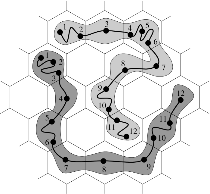
Figure 2: Illustration of the two-dimensional version of the lattice polymer model. In the upper polymer, interior monomers 2, 4, 6, 9, 10 and 11 can either diffuse along the polymer backbone, or move sideways; monomer 7 can join either 6 or 8; the end monomers 1 and 12 can move to any vacant nearest-neighbor site. In the lower polymer, interior monomers 3, 5, 6, 10 and 11 can either diffuse along the tube, or move sideways; monomer 1 can move to any vacant nearest-neighbor site, and monomer 12 can join its neighbor 11. All other monomers are not mobile.

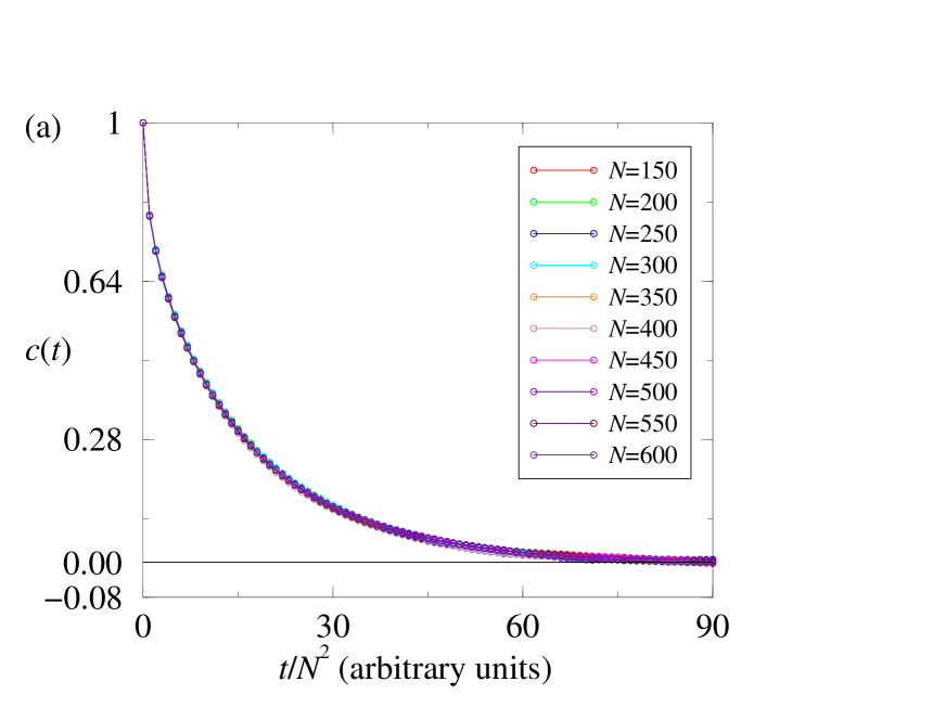
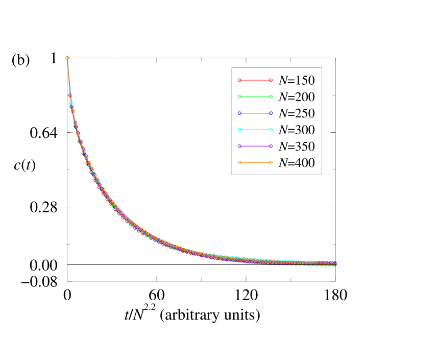
Figure 3: Collapse of $c(t)$ for different values of $N$, showing that the equilibration times for phantom and self-avoiding polymers scale as $N^{2}$ and $N^{1+2\nu}$ respectively. Here $N$ is the polymer length. (a) Data for phantom polymers, simulations were run with the same definition of time for all values of $N$; to achieve the data collapse, the times were then scaled by a factor $N^{2}$. (b) Data for self-avoiding polymers, simulations were run with the same definition of time for all values of $N$; to achieve the data collapse, the times were scaled by a factor $N^{1+2\nu}$ ($N^{2.2}$ to be precise). Note that the units of time are arbitrary and clearly not important for the scaling of polymer equilibration times.

II Our polymer model

Over the last years, we have developed a highly efficient simulation approach of polymer dynamics. This approach is made possible via a lattice polymer model, based on Rubinstein’s repton model rubinstein for a single reptating polymer, with the addition of sideways moves (Rouse dynamics) and entanglement. A detailed description of this lattice polymer model, its computationally efficient implementation and a study of some of its properties and applications can be found in Refs. heukelum03 ; LatMCmodel .

In this model, polymers consist of a sequential chain of monomers, living on a FCC lattice. Monomers adjacent in the string are located either in the same, or in neighboring lattice sites. The polymers are self-avoiding: multiple occupation of lattice sites is not allowed, except for a set of adjacent monomers. The polymers move through a sequence of random single-monomer hops to neighboring lattice sites. These hops can be along the contour of the polymer, thus explicitly providing reptation dynamics. They can also change the contour “sideways”, providing Rouse dynamics. Time in this polymer model is measured in terms of the number of attempted reptation moves. A two-dimensional version of our three-dimensional model is illustrated in fig. 2.

II.1 Influence of the accelerated reptation moves on polymer dynamics

From our experience with the model we already know that the dynamical properties are rather insensitive to the ratio of the rates for Rouse vs. reptation moves (i.e., moves that alter the polymer contour vs. moves that only redistribute the stored length along the backbone). Since the computational efficiency of the latter kind of moves is at least an order of magnitude higher, we exploit this relative insensitivity by attempting reptation moves $q$ times more often than Rouse moves; typical values are $q=1$, $5$ or 10, which correspond to a comparable amount of computational effort invested in both kinds of moves. Certainly, the interplay between the two kinds of moves is rather intricate wolt2 . Recent work by Drzewinski and van Leeuwen on a related lattice polymer model drz provides evidence that the dynamics is governed by $Nq^{-1/2}$, supporting our experience that, provided the polymers are sizable, one can boost one mechanism over the other quite a bit (even up to $q\sim N^{2}$) before the polymer dynamics changes qualitatively.

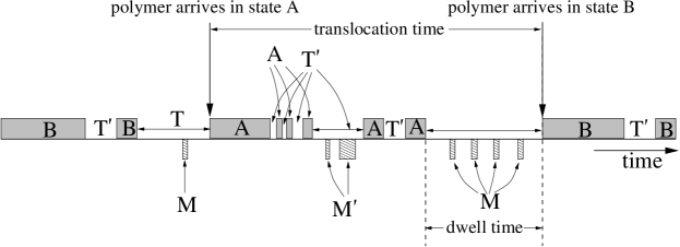
Figure 4: A typical translocation process of the polymer as for our system the polymers move repeatedly back and forth between cells A and B. See Fig. 1 and text for the definitions of the states A, B, T, M, $\mbox{T}^{\prime}$ and $\mbox{M}^{\prime}$.

In order to further check the trustworthiness of this model, we use it to study the equilibration properties of polymers with one end tethered to a fixed infinite wall (this problem relates rather directly to that of a translocating polymer: for a given monomer threaded into the pore, the two segments of the polymer on two sides of the membrane behave simply as two independent polymer chains; see Fig. 1). This particular problem, wherein polymer chains (of length $N$) undergo pure Rouse dynamics (i.e., no additional reptation moves) is a well-studied one: the equilibration time is known to scale as $N^{1+2\nu}$ for self-avoiding polymers and as $N^{2}$ for phantom polymers. To reproduce these results with our model we denote the vector distance of the free end of the polymer w.r.t. the tethered end at time $t$ by $\mathbf{e}(t)$, and define the correlation coefficient for the end-to-end vector as

$$c(t)=\frac{\langle\mathbf{e}(t)\cdot\mathbf{e}(0)\rangle-\langle\mathbf{e}(t)\rangle\cdot\langle\mathbf{e}(0)\rangle}{\sqrt{\langle\mathbf{e}^{2}(t)-\langle\mathbf{e}(t)\rangle^{2}\rangle\langle\mathbf{e}^{2}(0)-\langle\mathbf{e}(0)\rangle^{2}\rangle}}\,.$$ (1)

The angular brackets in Eq. (1) denote averaging in equilibrium. The $\bar{c}(t)$ quantities appearing in Fig. 3 have been obtained by the following procedure: we first obtain the time correlation coefficients $c(t)$ for $32$ independent polymers, and $\bar{c}(t)$ is a further arithmatic mean of the corresponding $32$ different time correlation coefficients. For different values of $N$ we measure $\bar{c}(t)$ for both self-avoiding and phantom polymers. When we scale the units of time by factors of $N^{2}$ and $N^{2.2}$ respectively for phantom and self-avoiding polymers, the $\bar{c}(t)$ vs. $t$ curves collapse on top of each other. This is shown in Fig. 3. Note here that $1+2\nu=2.175$, which is sufficiently close to $2.2$, and in simulations of self-avoiding polymers [Fig. 2(b)] we cannot differentiate between $1+2\nu$ and $2.2$.

III Translocation, dwell and unthreading times

Our translocation simulations are carried out only for self-avoiding polymers. For long polymers, full translocation simulations, i.e., having started in one of the cells (Fig. 1), finding the pore and distorting their shapes to enter the pore to finally translocate to the other side of the membrane are usually very slow. An uncoiled state, which the polymer has to get into in order to pass through the pore is entropically unfavourable, and therefore, obtaining good translocation statistics for translocation events is a time-consuming process. To overcome this difficulty, in Ref. wolt , we introduced three different time scales associated with translocation events: translocation time, dwell time and unthreading time. For the rest of this section, we refer the reader to Fig. 1.

III.1 Translocation and dwell times

In states A and B (Fig. 1), the entire polymer is located in cell A, resp. B. States M and ${\text{M}}^{\prime}$ are defined as the states in which the middle monomer is located exactly halfway between both cells. Finally, states T and ${\text{T}}^{\prime}$ are the complementary to the previous states: the polymer is threaded, but the middle monomer is not in the middle of the pore. The finer distinction between states M and T, resp. ${\text{M}}^{\prime}$ and ${\text{T}}^{\prime}$ is that in the first case, the polymer is on its way from state A to B or vice versa, while in the second case it originates in state A or B and returns to the same state. The translocation process in our simulations can then be characterized by the sequence of these states in time (Fig. 4). In this formulation, the dwell time $\tau_{d}$ is the time that the polymer spends in states T, while the translocation time $\tau_{t}$ is the time starting at the first instant the polymer reaches state A after leaving state B, until it reaches state B again. As found in Ref. wolt , $\tau_{d}$ and $\tau_{t}$ are related to each other by the relation

$$\tau_{t}\,=\,V\,\tau_{d}\,N^{1+\gamma-2\gamma_{1}}\,,$$ (2)

where $\gamma=1.1601$, $\gamma_{1}=0.68$ and $V$ is the volume of cell A or B (see Fig. 1).

III.2 Unthreading time and its relation to dwell time

The unthreading time $\tau_{u}$ is the average time that either state A or B is reached from state M (not excluding possible recurrences of state M). Notice that in the absence of a driving field, on average, the times to unthread to state A equals the the times to unthread to state B, due to symmetry. The advantage of introducing unthreading time is that when one measures the unthreading times, the polymer is at the state of lowest entropy at the start of the simulation and therefore simulations are fast and one can obtain good statistics on unthreading times fairly quickly. Additionally, the dwell and unthreading times are related to each other, as outlined below, and using this relation one is able to reach large values of $N$ for obtaining the scaling of the dwell time.

The main point to note that the dwell time can be decomposed into three parts as

$$\tau_{d}=\tau_{\mbox{\scriptsize A}\to\mbox{\scriptsize M}}\,+\,\tau_{\mbox{\scriptsize M}\looparrowright\mbox{\scriptsize M}}\,+\,\tau_{\mbox{\scriptsize M}\to\mbox{\scriptsize B}}\,,$$ (3)

whereas mean unthreading time can be decomposed into two parts as

$$\tau_{u}=\tau_{\mbox{\scriptsize M}\looparrowright\mbox{\scriptsize M}}\,+\,\tau_{\mbox{\scriptsize M}\to\mbox{\scriptsize B}}\,.$$ (4)

Here $\tau_{\mbox{\scriptsize A}\to\mbox{\scriptsize M}}$, $\tau_{\mbox{\scriptsize M}\looparrowright\mbox{\scriptsize M}}$ and $\tau_{\mbox{\scriptsize M}\to\mbox{\scriptsize B}}$ respectively are the mean first passage time to reach state M from state A, mean time between the first occurance at state M and the last occurance of state M with possible reoccurances of state M, and the mean first passage time to reach state B from state M without any reoccurance of state M. Since on average $\tau_{\mbox{\scriptsize A}\to\mbox{\scriptsize M}}=\tau_{\mbox{\scriptsize M}\to\mbox{\scriptsize B}}$ due to symmetry, and all quantities on the r.h.s. of Eqs. (3) and (4) are strictly positive, we arrive at the inequality

$$\tau_{u}<\tau_{d}<2\tau_{u}\,.$$ (5)

Since Eq. (5) is independent of polymer lengths, on average, the dwell time scales with $N$ in the same way as the unthreading time mistake .

IV Characterization of the anomalous dynamics of translocation and its relation to $\tau_{d}$

The reaction coordinate [the monomer number $s(t^{\prime})$, which is occupying the pore at time $t^{\prime}$] a convenient choice for the description of the microscopic movements of the translocating polymer, since the important time-scales for translocation can be obtained from the time evolution of the reaction coordinate $s(t^{\prime})$ as shown below. To delve deeper into its temporal behavior, we determine $P_{N,r}(s_{1},s_{2},t)$, the probability distribution that at time $t$ a polymer of length $N$ is in a configuration for which monomer $s_{1}$ is threaded into the pore, and the polymer evolves at time $t^{\prime}+t$ into a configuration in which monomer $s_{2}$ is threaded into the pore. The subscript $r$ denotes our parametrization for the polymer movement, as it determines the frequency of attempted reptation moves and the sideways (or Rouse) moves of the polymer. See Sec. II.1 for details.

To maintain consistency, all simulation results reported here in this section are for $q=10$, so we drop $q$ from all notations from here on. This value for $q$ is used in view of our experience with the polymer code: $q=10$ yields the fastest runtime of our code; this was the same value used in our earlier work wolt . As discussed in Sec. II.1, this value of $q$ does not change any physics.

First, we investigate the shape of these probability distributions for various values of $s_{1}$, $s_{2}$ and $t$, for different sets of $N$ and $r$ values. We find that as long as the $t$ values are such that neither $s_{1}$ nor $s_{2}$ are too close to the end of the polymer, $P_{N}(s_{1},s_{2},t)$ depends only on $(s_{2}-s_{1})$, but the centre of the distribution is slightly shifted w.r.t. the starting position $s_{1}$ by some distance that depends on $s_{1}$, $N$ and $q$. This is illustrated in Fig. 5, where (on top of each other) we plot $P_{N}(s_{1},s_{2},t)$ for $s_{1}=N/4,N/2$ and $3N/4$ at $t=100$ time units, for $N=400$, as well as the Gaussian distribution. Notice in fig. 5 that the distribution $P_{N}(s_{1},s_{2},t)$ differs slightly from Gaussian (the parameter for the Gaussian is calculated by least-square optimization). We find that this difference decreases with increasing values of $t$ (not shown in this paper).

We now define the mean $\langle[s_{2}-s_{1}]\rangle(s_{1},t)$ and the variance $\langle\Delta s^{2}(s_{1},t)\rangle$ of the distribution $P_{N}(s_{1},s_{2},t)$ as

$$\langle[s_{2}-s_{1}]\rangle(s_{1},t)\,=\,\int ds_{2}\,P_{N}(s_{1},s_{2},t)\,(s_{2}-s_{1});$$ (6)

$$\langle\Delta s^{2}(s_{1},t)\rangle\,=\,\int ds_{2}\,P_{N}(s_{1},s_{2},t)\times$$

$$\{(s_{2}-s_{1})^{2}-\,[\langle s_{2}-s_{1}\rangle(s_{1},t)]^{2}\}\,,$$

where the quantities within parenthesis on the l.h.s. of Eq. (6) denote the functional dependencies of the mean and the standard deviation of $(s_{2}-s_{1})$. We also note here that we have checked the skewness of $P_{N}(s_{1},s_{2},t)$, which we found to be zero within our numerical abilities, indicating that $P_{N}(s_{1},s_{2},t)$ is symmetric in $(s_{2}-s_{1})$.

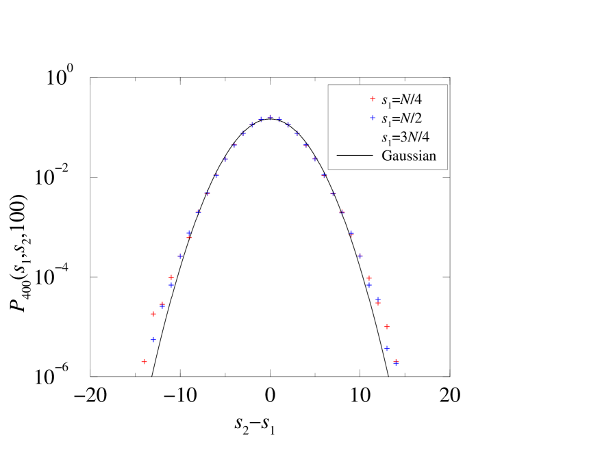
Figure 5: $P_{N}(s_{1},s_{2},t)$ for $N=400$, at $t=100$. Note the data collapse when plotted as a function of $(s_{2}-s_{1})$. The distribution differs slightly from Gaussian.

In principle, both the mean and the standard deviation of $(s_{2}-s_{1})$ can be used to obtain the scaling of $\tau_{d}$ with $N$, but the advantage of using $\langle\Delta s^{2}(s_{1},t)\rangle$ for this purpose is that, as shown in Fig. 5, it is independent of $s_{1}$, so from now on, we drop $s_{1}$ from its argument. Since unthreading process starts at $s_{1}=N/2$, the scaling of $\tau_{d}$ with $N$ is easily obtained by using the relation

$$\langle\Delta s^{2}(\tau_{d})\rangle\sim N^{2}\,,$$ (7)

in combination with the fact that the scalings of $\tau_{d}$ and $\tau_{u}$ with $N$ behave in the same way [inequality (5)]. Note here that Eq. (7) uses the fact that for an unthreading process the polymer only has to travel a length $N/2$ along its contour in order to leave the pore.

IV.1 The origin of anomalous dynamics and the relaxation of excess monomer density near the pore during translocation

The key step in quantitatively formulating the anomalous dynamics of translocation is the following observation: a translocating polymer comprises of two polymer segments tethered at opposite ends of the pore that are able to exchange monomers between them through the pore; so each acts as a reservoir of monomers for the other. The velocity of translocation $v(t)=\dot{s}(t)$, representing monomer current, responds to $\phi(t)$, the imbalance in the monomeric chemical potential across the pore acting as “voltage”. Simultaneously, $\phi(t)$ also adjusts in response to $v(t)$. In the presence of memory effects, they are related to each other by $\phi(t)=\int_{0}^{t}dt^{\prime}\mu(t-t^{\prime})v(t^{\prime})$ via the memory kernel $\mu(t)$, which can be thought of as the (time-dependent) ‘impedance’ of the system. Supposing a zero-current equilibrium condition at time $0$, this relation can be inverted to obtain $v(t)=\int_{0}^{t}dt^{\prime}a(t-t^{\prime})\phi(t^{\prime})$, where $a(t)$ can be thought of as the ‘admittance’. In the Laplace transform language, $\tilde{\mu}(k)=\tilde{a}^{-1}(k)$, where $k$ is the Laplace variable representing inverse time. Via the fluctuation-dissipation theorem, they are related to the respective autocorrelation functions as $\mu(t-t^{\prime})=\langle\phi(t)\phi(t^{\prime})\rangle_{v=0}$ and $a(t-t^{\prime})=\langle v(t)v(t^{\prime})\rangle_{\phi=0}$.

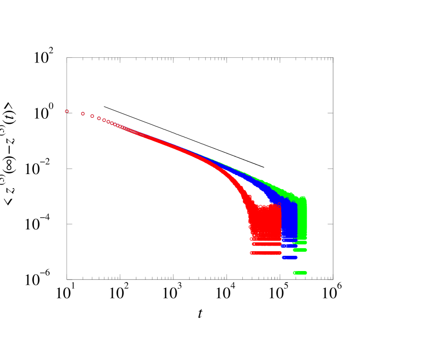
Figure 6: (colour online) Simulation results for the average chain tension component perpendicular to the membrane proxied by $\langle z^{(5)}(\infty)-z^{(5)}(t)\rangle$ following monomer injection at the pore corresponding to $v(t)=p\delta(t)$, with $p=10$. See text for details. Red circles: $N/2=50$, blue circles: $N/2=100$, green circles: $N/2=150$, solid black line: $t^{-(1+\nu)/(1+2\nu)}$ with $\nu=0.588$ for self-avoiding polymers. The steeper drop at large times correspond to the exponential decay $\exp(-t/\tau_{R})$ (we have checked this, but have not shown in this letter).

The behaviour of $\mu(t)$ may be obtained by considering the polymer segment on one side of the membrane only, say the right, with a sudden introduction of $p$ extra monomers at the pore, corresponding to impulse current $v(t)=p\delta(t)$. We then ask for the time-evolution of the mean response $\langle\delta\Phi^{(r)}(t)\rangle$, where $\delta\Phi^{(r)}(t)$ is the shift in chemical potential for the right segment of the polymer at the pore. This means that for the translocation problem (with both right and left segments), we would have $\phi(t)=\delta\Phi^{(r)}(t)-\delta\Phi^{(l)}(t)$, where $\delta\Phi^{(l)}(t)$ is the shift in chemical potential for the left segment at the pore due to an opposite input current to it.

We now argue that this mean response, and hence $\mu(t)$, takes the form $\mu(t)\sim t^{-\alpha}\exp(-t/\tau_{R})$. The terminal exponential decay $\exp(-t/\tau_{R})$ is expected from the relaxation dynamics of the entire right segment of the polymer with one end tethered at the pore [see Fig. 3(b)]. To understand the physics behind the exponent $\alpha$, we use the well-established result for the relaxation time $t_{n}$ for $n$ self-avoiding Rouse monomers scaling as $t_{n}\sim n^{1+2\nu}$. Based on the expression of $t_{n}$, we anticipate that by time $t$ the extra monomers will be well equilibrated across the inner part of the chain up to $n_{t}\sim t^{1/(1+2\nu)}$ monomers from the pore, but not significantly further. This internally equilibrated section of $n_{t}+p$ monomers extends only $r(n_{t})\sim n_{t}^{\nu}$, less than its equilibrated value $\left(n_{t}+p\right)^{\nu}$, because the larger scale conformation has yet to adjust: the corresponding compressive force from these $n_{t}+p$ monomers is expected by standard polymer scaling degennes to follow $f/(k_{B}T)\sim\delta r(n_{t})/r^{2}(n_{t})\sim\nu p/\left[n_{t}r(n_{t})\right]\sim t^{-(1+\nu)/(1+2\nu)}$. This force $f$ must be transmitted to the membrane, through a combination of decreased tension at the pore and increased incidence of other membrane contacts. The fraction borne by reducing chain tension at the pore leads us to the inequality $\alpha\geq(1+\nu)/(1+2\nu)$, which is significantly different from (but compatible with) the value $\alpha_{1}=2/(1+2\nu)$ required to obtain $\tau_{d}\sim\tau_{R}$ . It seems unlikely that the adjustment at the membrane should be disproportionately distributed between the chain tension at the pore and other membrane contacts, leading to the expectation that the inequality above is actually an equality.

We have confirmed this picture by measuring the impedance response through simulations. In Ref. forced , two of us have shown that the centre-of-mass of the first few monomers is an excellent proxy for chain tension at the pore and we assume here that this further serves as a proxy for $\delta\Phi$. Based on this idea, we track $\langle\delta\Phi^{(r)}(t)\rangle$ by measuring the distance of the average centre-of-mass of the first $5$ monomers from the membrane, $\langle z^{(5)}(t)\rangle$, in response to the injection of extra monomers near the pore at time $0$. Specifically we consider the equilibrated right segment of the polymer, of length $N/2-10$ (with one end tethered at the pore), adding $p=10$ extra monomers at the tethered end of the right segment at time $0$, corresponding to $p=10$, bringing its length up to $N/2$. Using the proxy $\langle z^{(5)}(t)\rangle$ we then track $\langle\delta\Phi^{(r)}(t)\rangle$. The clear agreement between the exponent obtained from the simulation results with the theoretical prediction of $\alpha=(1+\nu)/(1+2\nu)$ can be seen in Fig. 6. We have checked that the sharp deviation of the data from the power law $t^{-(1+\nu)/(1+2\nu)}$ at long times is due to the asymptotic exponential decay as $\exp(-t/\tau_{R})$, although this is not shown in the figure.

Having thus shown that $\mu(t)\sim t^{-\frac{1+\nu}{1+2\nu}}\exp(-t/\tau_{R})$, we can expect that the translocation dynamics is anomalous for $t<\tau_{R}$, in the sense that the mean-square displacement of the monomers through the pore, $\langle\Delta s^{2}(t)\rangle\sim t^{\beta}$ for some $\beta<1$ and time $t<\tau_{R}$, whilst beyond the Rouse time it becomes simply diffusive. The value $\beta=\alpha=\frac{1+\nu}{1+2\nu}$ follows trivially by expressing $\langle\Delta s^{2}(t)\rangle$ in terms of (translocative) velocity correlations $\left\langle v(t)v(t^{\prime})\right\rangle$, which (by the Fluctuation Dissipation theorem) are given in terms of the time dependent admittance $a(t-t^{\prime})$. and hence inversely in terms of the corresponding impedance.

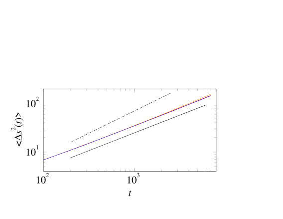
Figure 7: (colour online) Double-logarithmic plot of the mean squared displacement of the reaction coordinate $\langle\Delta s^{2}(t)\rangle$ as a function of time $t$, for $N=100$ (orange), 200 (red) and 500 (blue). The thick black line indicates the theoretically expected slope corresponding to $\langle\Delta s^{2}(t)\rangle\sim t^{(1+\nu)/(1+2\nu)}$. The dashed black line corresponds to $\langle\Delta s^{2}(t)\rangle\sim t^{2/(1+2\nu)}$, which would have been the slope of the $\langle\Delta s^{2}(t)\rangle$ vs. $t$ curve in a double-logarithmic plot, if $\tau_{d}$ were to scale as $\tau_{R}\sim N^{1+2\nu}$.

Indeed, as shown in Fig. 7, a double-logarithmic plot of $\langle\Delta s^{2}(t)\rangle$ vs. $t$ is consistent with $\langle\Delta s^{2}(t)\rangle\sim t^{(1+\nu)/(1+2\nu)}$. The behaviour of $\langle\Delta s^{2}(t)\rangle$ at short times is an artifact of our model: at short times reptation moves dominate, leading to a transport mechanism for “stored lengths” rubinstein along the polymer’s contour in which individual units of stored length cannot pass each other. As a result, the dynamics of $s(t)$, governed by the movement of stored length units across the pore, is equivalent to a process known as “single-file diffusion” on a line, characterized by the scaling $\langle\Delta s^{2}(t)\rangle\sim t^{1/2}$ (not shown here). At long times the polymer tails will relax, leading to $\langle\Delta s^{2}(t)\rangle\sim t$ for $t>\tau_{R}$. The presence of two crossovers, the first one from $\langle\Delta s^{2}(t)\rangle\sim t^{1/2}$ to $\langle\Delta s^{2}(t)\rangle\sim t^{(1+\nu)/(1+2\nu)}$ and the second one from $\langle\Delta s^{2}(t)\rangle\sim t^{(1+\nu)/(1+2\nu)}$ to $\langle\Delta s^{2}(t)\rangle\sim t$ at $t\approx\tau_{R}$, complicates the precise numerical verification of the exponent $(1+\nu)/(1+2\nu)$. However, as shown in Fig. 7, there is an extended regime in time at which the quantity $t^{-(1+\nu)/(1+2\nu)}\langle\Delta s^{2}(t)\rangle$ is nearly constant.

The subdiffusive behaviour $\langle\Delta s^{2}(t)\rangle\sim t^{\frac{1+\nu}{1+2\nu}}$ for $t<\tau_{R}$, combined with the diffusive behaviour for $t\geq\tau_{R}$ leads to the dwell time scaling as $\tau_{d}\sim N^{2+\nu}$, based on the criterion that $\sqrt{\langle\Delta s^{2}(\tau_{d})\rangle}\sim N$. The dwell time exponent $2+\nu\simeq 2.59$ is in acceptable agreement with the two numerical results on $\tau_{d}$ in 3D as mentioned in the introduction of this letter, and in Table I below we present new high-precision simulation data in support of $\tau_{d}\sim N^{2+\nu}$, in terms of the median unthreading time. The unthreading time $\tau_{u}$ is defined as the time for the polymer to leave the pore with $s(t=0)=N/2$ and the two polymer segments equilibrated at $t=0$. Both $\tau_{u}$ and $\tau_{d}$ scale the same way, since $\tau_{u}<\tau_{d}<2\tau_{u}$ [see Eq. (5)].

$N$	$\tau_{u}$	$\tau_{u}/N^{2+\nu}$
100	65136	0.434
150	183423	0.428
200	393245	0.436
250	714619	0.445
300	1133948	0.440
400	2369379	0.437
500	4160669	0.431

Table I: Median unthreading time over 1,024 runs for each $N$.

Our results have two main significant implications:

• Even in the limit of small (or negligible) pore friction, equilibration time scale of a polymer is smaller than its dwell time scale. Yet, quasi-equilibrium condition cannot be assumed as the starting point to analyze the dynamics of unbiased translocation, as has been done in the mean-field theories.

• Since $\alpha=(1+\nu)/(1+2\nu)<1$, the diffusion in reaction-coordinate space is anomalous. This means that the dynamics of the translocating polymer in terms of its reaction co-ordinate cannot be captured by a Fokker-Planck equation in the limit of small (or negligible) pore friction.

  In view of our results, a Fokker-Planck type equation [such as a fractional Fokker-Planck equation (FFPE)] to describe the anomalous dynamics of a translocating polymer would definitely need input from the physics of polymer translocation. It therefore remains to be checked that the assumptions underlying a FFPE does not violate the basic physics of a translocating polymer.

IV.2 Comparison of our results with the theory of Ref. dubbeldam

We now reflect on the theory presented in Ref. dubbeldam .

We have defined $\tau_{d}$ as the pore-blockade time in experiments; i.e., if we define a state of the polymer with $s(t)=0$ as ‘0’ (polymer just detached from the pore on one side), and with $s(t)=N$ as ‘N’, then $\tau_{d}$ is the first passage time required to travel from state 0 to state N without possible reoccurances of state 0. In Ref. dubbeldam , the authors attach a bead at the $s=0$ end of the polymer, preventing it from leaving the pore; and their translocation time ($\tau_{v}$ hereafter) is defined as the first passage time required to travel from state 0 to state N with reoccurances of state 0. This leads them to express $\tau_{v}$ in terms of the free energy barrier that the polymer encounters on its way from state 0 to $s=N/2$, where the polymer’s configurational entropy is the lowest. Below we settle the differences between $\tau_{v}$ of Ref. dubbeldam and our $\tau_{d}$.

Consider the case where we attach a bead at $s=0$ and another at $s=N$, preventing it from leaving the pore. Its dynamics is then given by the sequence of states, e.g.,

$$...\mbox{N \!x\! m\! x}\overbrace{\mbox{0 \!x${}^{\prime}$0 \!x${}^{\prime}$m${}^{\prime}$x${}^{\prime}$m${}^{\prime}$x${}^{\prime}$0 \!x${}^{\prime}$}\underbrace{\mbox{0 \!x \!m \!x \!m \!x \!m \!x \!N}}_{\tau_{d}}}^{\tau_{v}}\mbox{x${}^{\prime}$N}...$$

where the corresponding times taken ($\tau_{v}$ and $\tau_{d}$) are indicated. At state x and x^′ the polymer can have all values of $s$ except $0,N/2$ and $N$; and at states m and m^′, $s=N/2$. The notational distinction between primed and unprimed states is that a primed state can occur only between two consecutive states 0, or between two consecutive states N, while an unprimed state occurs only between state 0 and state N. A probability argument then leads us to

$$\frac{\tau_{v}}{\tau_{d}}\,=\,\frac{1}{p_{\text{x}}+p_{\text{m}}}\,=\,\frac{f_{\text{x}}\,(1+f_{\text{m}})}{(p_{\text{m}}+p_{\text{m${}^{\prime}$}})f_{\text{m}}(1+f_{\text{x}})}\,,$$ (8)

where $p_{\text{m}}$, $p_{\text{m}^{\prime}}$ and $p_{\text{x}}$ are the probabilities of the corresponding states, $f_{\text{m}}=p_{\text{m}}/p_{\text{m}^{\prime}}$ and $f_{\text{x}}=p_{\text{m}}/p_{\text{x}}$. Since the partition sum of a polymer of length $n$ with one end tethered on a membrane is given by $Z_{n}\sim\lambda^{n}~{}n^{\gamma_{1}-1}$ with $\lambda$ a non-universal constant and $\gamma_{1}=0.68$ diehla , we have $p_{\text{m}}+p_{\text{m}^{\prime}}=Z_{N/2}^{2}/\left[\sum_{s=0}^{N}Z_{s}Z_{N-s}\right]\sim 1/N$. Similarly, $f_{\text{x}}\sim 1/N$ wolt . Finally, $f_{\text{m}}\approx 1$ note yields $\tau_{v}\sim\tau_{d}$.

We have thus shown that the free energy barrier does not play a role for $\tau_{v}$, implying that the theoretical expression for $\tau_{v}$ in Ref. dubbeldam cannot be correct. The numerical result $\tau_{v}\sim N^{2.52\pm 0.04}$ in Ref. dubbeldam , however, confirms our theoretical expression $\tau_{d}\sim N^{2+\nu}$.

V Conclusion

To conclude, we have shown that for the swollen Rouse chain, translocation is sub-diffusive up the configurational relaxation time (Rouse time) of the molecule, after which it has a further Fickian regime before the longer dwell time is exhausted: the mean square displacement along the chain is described by $\langle\Delta s^{2}(t)\rangle\sim t^{(1+\nu)/(1+2\nu)}$ up to $t\sim N^{1+2\nu}$, after which $\langle\Delta s^{2}(t)\rangle\sim t$. Consequently, the mean dwell time scales as $\tau_{d}\sim N^{2+\nu}$.

In future work, we will study the role of hydrodynamics. Rouse friction may be an appropriate model for the dynamics of long biopolymers in the environment within living cells, if it is sufficiently gel-like to support screened hydrodynamics on the timescale of their configurational relaxation. However, we should also ask what is expected in the other extreme of unscreened (Zimm) hydrodynamics. For our theoretical discussion the key difference is that, instead of the Rouse time $\tau_{R}$, in the Zimm case the configurational relaxation times scale with $N$ according to $\tau_{\text{Zimm}}\sim N^{3\nu}$ in 3D, which upon substitution into our earlier argument would gives the lower bound value $\alpha=(1+\nu)/(3\nu)$ for the time exponent of the impedance, leading to $\tau_{d}\sim N^{1+2\nu}$ (whose resemblance to the Rouse time is a coincidence — note that with hydrodynamics Rouse time loses all relevance). These results, however, do need to be verified by simulations incorporating hydrodynamics.

References

- (1) B. Dreiseikelmann, Microbiol. Rev. 58, 293 (1994).
- (2) J. P. Henry et al., J. Membr. Biol. 112, 139 (1989).
- (3) J. Akimaru et al., PNAS USA 88, 6545 (1991).
- (4) D. Goerlich and T. A. Rappaport, Cell 75, 615 (1993).
- (5) G. Schatz and B. Dobberstein, Science 271, 1519 (1996).
- (6) J. J. Nakane, M. Akeson, A. Marziali, J. Phys.: Cond. Mat. 15, R1365 (2003).
- (7) I. Szabò et al. J. Biol. Chem. 272, 25275 (1997).
- (8) B. Hanss et al., PNAS USA 95, 1921 (1998).
- (9) Yun-Long Tseng et al., Molecular Pharm. 62, 864 (2002).
- (10) W. T. Wickner and H. F. Lodisch, Science 230, 400 (1995).
- (11) S. M. Simon and G. Blobel, Cell 65, 1 (1991); D. Goerlich and I. W. Mattaj, Science 271, 1513 (1996); K. Verner and G. Schatz, Science 241, 1307 (1988).
- (12) P. J. Sung and W. Park, Phys. Rev. E 57, 730 (1998); M. Muthukumar, Phys. Rev. Lett. 86, 3188 (2001).
- (13) P. J. Sung and W. Park, Phys. Rev. Lett. 77, 783 (1996); M. Muthukumar, J. Chem. Phys. 111, 10371 (1999).
- (14) D. K. Lubensky and D. R. Nelson, Biophys. J. 77, 1824 (1999); P. J. Park and W. Sung, J. Chem. Phys. 108, 3013 (1998); E. Slonkina and A. B. Kolomeisky, J. Chem. Phys. 118, 7112 (2003).
- (15) J. K. Wolterink, G. T. Barkema and D. Panja, Phys. Rev. Lett. 96, 208301 (2006).
- (16) J. Kasianowicz et al., PNAS USA 93, 13770 (1996); E. Henrickson et al., Phys. Rev. Lett. 85, 3057 (2000); A Meller et al., Phys. Rev. Lett. 86, 3435 (2001); M. Akeson et al., Biophys. J. 77, 3227 (1999); A. Meller et al., PNAS USA 97, 1079 (2000); A. J. Storm et al., Nanoletters 5, 1193 (2005).
- (17) J. Chuang et al., Phys. Rev. E 65, 011802 (2002); Y. Kantor and M. Kardar, Phys. Rev. E 69, 021806 (2004).
- (18) I. Huopaniemi, K. Luo, T. Ala-Nissila, S.-C. Ying, J. Chem. Phys. 125 124901 (2006).
- (19) The exponent is also known as the Flory exponent and sometimes also referred to as the “swelling exponent”.
- (20) R. Metzler and J. Klafter, Biophys. J. 85 2776 (2003).
- (21) J. L. A. Dubbeldam, A. Milchev, V. G. Rostianshvili and T. A. Vilgis, e-print archive cond-mat/070166.
- (22) Strictly speaking, in this expression should be replaced by the characteristic equilibration time of a tethered polymer with length of ; since both scale as , we use here, favouring notational simplicity.
- (23) A. van Heukelum and G. T. Barkema, J. Chem. Phys. 119, 8197 (2003).
- (24) A. van Heukelum et al., Macromol. 36, 6662 (2003); J. Klein Wolterink et al., Macromol. 38, 2009 (2005).
- (25) J. Klein Wolterink and G. T. Barkema, Mol. Phys. 103, 3083 (2005).
- (26) A. Drzewinski and J.M.J. van Leeuwen, e-print archive cond-mat/0609281 (2006).
- (27) In Ref. wolt we overlooked the term of Eq. (3) to (mistakenly) deduce . Nevertheless, due to the independence of Eq. (5) on our results for the scaling of in Ref. wolt remain unaffected.
- (28) D. Panja and G. T. Barkema, cond-mat/0706.3969.
- (29) P.-G. de Gennes, Scaling concepts in polymer physics (Cornell University Press, New York, 1979).
- (30) M. Rubinstein, Phys. Rev. Lett. 59, 1946 (1987); T. A. J. Duke, Phys. Rev. Lett. 62, 2877 (1989).
- (31) H.W. Diehla and M. Shpot, Nucl. Phys. B 528, 595 (1998).
- (32) is a number slightly smaller than : if the polymer reaches from state 0, due to the memory effects, it will have slightly higher chance to go back to state 0 rather than to proceed to state N wolt .