New Numerical Results Indicate a Half-Filling SU(4) Kondo State in Carbon Nanotubes

Abstract

Numerical calculations simulate transport experiments in carbon nanotube quantum dots (P. Jarillo-Herrero et. al, Nature 434, 484 (2005)), where a strongly enhanced Kondo temperature ${\rm T_{K}}\approx 8.0~{}{\rm K}$ was associated with the SU(4) symmetry of the Hamiltonian at quarter-filling for an orbitally double-degenerate single-occupied electronic shell. Our results clearly suggest that the Kondo conductance measured for an adjacent shell with ${\rm T_{K}}\approx 16.0~{}{\rm K}$, interpreted as a singlet-triplet Kondo effect, can be associated instead to an SU(4) Kondo effect at half-filling. Besides presenting spin-charge Kondo screening similar to the quarter-filling SU(4), the half-filling SU(4) has been recently associated to very rich physical behavior, including a non-Fermi-liquid state (M. R. Galpin et al., Phys. Rev. Lett. 94, 186406 (2005)).

I Introduction

The synthesis of nanostructures such as quantum dots (QDs) has attained a high level of sophistication, allowing control over systems displaying complex many-body properties. Recently, the observation of the Kondo effect in orbitally degenerate carbon nanotube (CNT) QDs by Jarillo-Herrero et al. jarillo has renewed interest in the so-called SU(4) Kondo effect. Early measurements of orbital Kondo effect in double QDs can be found in work by U. Wilhelm et al. wilhelm , while more recent results are reported in A. W. Holleitner et al. holleitner . However, no conclusive evidence for an SU(4) Kondo effect in double QDs has been established. To date, besides the results in CNT QDs jarillo , clear evidence of SU(4) Kondo has been reported in vertical QDs sasaki1 . Early theoretical work can be found in T. Pohjola et al. pohjola and in L. Borda et al. borda , while a review of SU(4) Kondo in nanostructures was written by G. Zarand zarand . Recently, a flurry of theoretical results exploring more detailed aspects of the SU(4) Kondo effect have been presented for a diversity of setups lehur . Quite recent transport measurements in ambipolar semiconducting CNT QDs gleb report conductance results for a large sequence of electronic shells in the QD, with clear indication of SU(4) states.

Besides the fact that the Kondo temperature of an SU(4) Kondo state is in general at least one order of magnitude higher than the traditional SU(2) Kondo temperatures note1 , there is also great interest in studying mesoscopic systems with two or more interacting SU(4) Kondo impurities, since this could shed light into the puzzling behavior of some bulk systems displaying the orbitally degenerate Kondo effect. For instance, $\rm Ce_{x}La_{1-x}B_{6}$, a well-known Kondo system with orbitally degenerate impurities, presents a magnetic phase diagram which still defies theoretical description iroi . Another intriguing aspect recently discussed is the possibility of orbitally degenerate QDs being Jahn-Teller active toonen . In addition, the simultaneous Kondo screening of charge and spin, resulting in a many-body entangled state for these two degrees of freedom goldhaber , points to the exciting possibility of observing new many-body states.

The interpretation of the CNT experimental results jarillo through numerical calculations has concentrated specifically on quarter-filling (QF) (1 electron occupying the topmost electronic shell in the QD) aguado1 ; aguado2 . In reality, most of the theoretical research on the SU(4) Kondo effect in QDs has concentrated on the QF regime, with the sole exception of the work by M. R. Galpin et al. galpin1 ; galpin2 , where NRG calculations analyzed the properties of the SU(4) Kondo effect at half-filling (HF), i.e., with 2 electrons in the topmost electronic shell.

In this paper, motivated by these interesting new possibilities regarding the SU(4) Kondo effect in QDs, the authors will use a recently developed numerical method, called Embedded Cluster Approximation (ECA) method , to reanalyze the conductance measurements performed in a CNT QD by Jarillo-Herrero et al. jarillo and also to extend the already mentioned QF aguado1 ; aguado2 and HF galpin1 ; galpin2 results to all fillings, paying special attention to the robustness of the SU(4) state in respect to the tunneling properties of the QD. The rest of the paper is organized as follows: The model used is presented in section II, where the ECA method will be briefly described. As an illustration of the capabilities of the ECA method, in section III the authors qualitatively reproduce the NRG results presented by Galpin et al. galpin1 . In section IV it will be shown that the state where the orbital degree of freedom is not conserved upon tunneling (see Fig. 1), also called Two-Level SU(2) (2LSU(2)), is qualitatively different from the SU(4) state (where the orbital degree of freedom is conserved) even at zero magnetic field. Also in section IV, the authors will analyze the transition between SU(4) and 2LSU(2) states, comparing our results to previously published results aguado2 . In section V, by realizing that there is spin-charge entanglement also at HF, the authors will suggest that the conductance of one of the electronic shells observed in the experiments (the third shell) can be associated to an SU(4) Kondo effect, offering an alternative to the single-triplet effect sasaki interpretation suggested by Jarillo-Herrero et al. jarillo . The authors also note that recent experimental results by Makarovski et al. gleb n CNT QDs give support to our HF SU(4) Kondo interpretation. This new interpretation of the CNT results jarillo implies that the rich physics unveiled by the NRG results of Galpin et al. galpin1 , also confirmed by our results (see Fig. 2), could, at least in principle, be probed in CNT QDs. To further support our interpretation, in section V results in agreement with the experiments will be presented for a magnetic field applied along the axis of the CNT jarillo ; jarillo2 . In section VI the conclusions are presented.

II Model

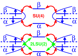
Figure 1: Schematic representation of the system being analyzed. Top: Hopping matrix elements (in red) conserving the orbital degree of freedom (indicated by the blue arrows) lead to a Hamiltonian with SU(4) symmetry. Bottom: The orbital degree of freedom is not conserved upon tunneling (notice the green arrows), leading to a so-called 2LSU(2) state (see reference aguado2, for a detailed discussion of this transition at QF).

The CNT QD will be modeled by an orbitally degenerate Anderson impurity coupled to leads with two conduction channels:

$$H_{\rm d}=\sum_{\sigma;\lambda=\alpha,\beta}\left[{U\over 2}n_{\lambda\sigma}n_{\lambda\bar{\sigma}}+V_{g}n_{\lambda\sigma}\right]+U^{\prime}\sum_{\sigma\sigma^{\prime}}n_{\alpha\sigma}n_{\beta\sigma^{\prime}},$$ (1)

$$H_{\rm leads} = t\sum_{l=R,L}\sum_{\sigma;\lambda=\alpha,\beta;i}\left[c_{l_{\lambda}i\sigma}^{\dagger}c_{l_{\lambda}i+1\sigma}+\mbox{h.c.}\right],$$ (2)

$$H_{\rm int} = \sum_{l=R,L}\sum_{\lambda;\lambda^{\prime};\sigma}t_{\lambda\lambda^{\prime}}\left[d_{\lambda\sigma}^{\dagger}c_{l_{\lambda^{\prime}}0\sigma}+\mbox{h.c.}\right],$$ (3)

where $H_{\rm d}$ describes the orbitally degenerate Anderson impurity, subjected to a gate potential $V_{g}$, and the second and third equations describe the leads and their interaction with the CNT QD, respectively. More specifically, $\lambda=\alpha,\beta$ are two degenerate orbitals associated to the wrapping mode (clockwise or counterclockwise) of the electron propagation along the axial direction of the CNT minot , while $d_{\alpha\sigma}$ ($d_{\beta\sigma}$) annihilates an electron with spin $\sigma$ in the $\alpha$ ($\beta$) orbital in the CNT and $c_{l_{\alpha}i\sigma}$ ($c_{l_{\beta}i\sigma}$) annihilates an electron with spin $\sigma$ in the i-th site of the $\alpha$ ($\beta$) channel in the $l=R,L$ (right or left) lead channels . We introduce intra- and inter-orbital Coulomb repulsions $U$ and $U^{\prime}$, respectively. To decrease the number of parameters in the model, the hopping matrix elements connecting the CNT QD to the leads (eq. 3) are the same at left and right, and assumed to follow the equalities $t_{\alpha\alpha}=t_{\beta\beta}=t^{\prime}$ (red arrows in Fig. 1) and $t_{\alpha\beta}=t_{\beta\alpha}=t^{\prime\prime}$ (green arrows in Fig. 1). As discussed in references aguado1, and aguado2, , when $t^{\prime}$ is finite and $t^{\prime\prime}=0$, one has an SU(4) Kondo state. On the other hand, when $t^{\prime}=t^{\prime\prime}$, one has the so-called 2LSU(2) Kondo state. As discussed in the Supplementary Information in reference jarillo, , there are fundamental differences between these two states. The 2LSU(2) Kondo effect is more akin to the singlet-triplet Kondo effect sasaki , where spin and orbital degrees of freedom have different roles: only the spin degree of freedom is screened by the conduction electrons, while the degenerate orbital levels just contribute to the increase in the possible number of co-tunneling processes, leading to an enhanced Kondo temperature. In this case, the orbital degree of freedom is not screened by the conduction electrons. On the other hand, in the SU(4) state, spin and orbital degrees of freedom participate in the same footing. Both of them are screened by the conduction electrons, and if the screening of one of the degrees of freedom is somehow suppressed, the system is then left in an SU(2) Kondo effect stemming from the other degree of freedom.

To calculate the conductance $G$, using the Keldysh formalism Meir-cnd , a cluster containing the orbitally degenerate Anderson impurity plus a few sites of the leads is solved exactly, the Green functions are calculated, and the leads are then incorporated through a Dyson Equation embedding procedure method . All the results shown were obtained for (in units of $t$) $U=0.5$, $t^{\prime}=0.2$, zero-bias, and zero temperature. The value of $t^{\prime\prime}$ varies between zero and $t^{\prime}$ and most of the results shown are for $U^{\prime}=U$. When a magnetic field is applied along the CNT axis, besides the Zeeman splitting coming from the spin degree of freedom, the orbital levels behave as a pseudo-spin $1/2$ and are also split minot : $H_{\rm Zeeman}=B\left[\mu_{orb}\sum_{\sigma}\left(n_{\beta\sigma}-n_{\alpha\sigma}\right)+\mu_{sp}\sum_{\lambda}\left(n_{\lambda+}-n_{\lambda-}\right)\right]$. As reported by Jarillo-Herrero et al. jarillo , the orbital magnetic moment $\mu_{orb}$ experimentally measured is such that the orbital splitting is one order of magnitude larger than the spin splitting. For the actual simulation of the experimental results (Figs. 6 and 7), the degeneracy of the orbital levels will be raised by introducing a small energy splitting $\delta E$ splitting .

III Comparison with NRG results at Half-Filling

Before presenting the main results in this work, the authors will show that ECA can qualitatively reproduce the NRG results of Galpin et al. (Fig. 2). Besides showing that ECA captures correctly the physics of the model, this qualitative agreement shows that the NRG low-energy results in ref. galpin1, are robust, suggesting that they could be observable if one can find an experimental realization of the SU(4) state at HF (more on that below).

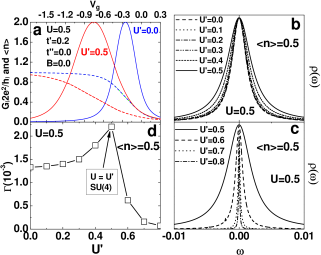
Figure 2: (a) Blue: Conductance $G$ (solid) and average occupancy $\left<n\right>$ per spin orientation, per orbital (dashed) obtained when the two orbital levels are not correlated ($U^{\prime}=0.0$). Red: Same as blue curves, but now the orbital levels are correlated ($U^{\prime}=0.5$). In both cases, $U=0.5$, $t^{\prime}=0.2$, and $t^{\prime\prime}=0.0$. (b) Variation with $U^{\prime}$ of the LDOS at HF, from $U^{\prime}=0.0$ (SU(2)$\times$SU(2), bottom curve) to $U^{\prime}=U=0.5$ (SU(4), top curve). (c) Same as in (b), but now for $U^{\prime}\geq U$ ($U^{\prime}=U$ top curve). (d) Variation with $U^{\prime}$ of the width of the peaks ($\Gamma$) in (b) and (c), which is proportional to $T_{K}$. The qualitative behavior matches the results presented in reference galpin1, .

Figure 2 displays the influence of $U^{\prime}$ (Coulomb repulsion between the two orbital levels) over the conductance in the case where the two channels are independent ($t^{\prime\prime}=0.0$), i. e., a transmitted electron that tunnels into the CNT QD coming from the $\alpha$ ($\beta$)-channel in the left lead, can only tunnel out through the $\alpha$ ($\beta$)-channel in the right lead. The blue curves ($U^{\prime}=0$) in Fig. 2a are representative of two independent spin SU(2) Kondo effects (associated to each channel) which are simply added together. In this case, each channel magnetically screens the spin situated on the level to which it is connected ($\alpha$ or $\beta$). This situation changes if the orbital levels are correlated with each other (finite $U^{\prime}$, red curves), i. e., in the SU(4) state. As can be seen in Fig. 2b (at HF, i.e., $\left<n\right>=0.5$), the width of the Kondo resonance in the local density of states (LDOS) becomes larger as $U^{\prime}$ increases, indicating an enhancement of $T_{K}$: in the SU(4) state at HF, both degrees of freedom (spin and orbital) are participating in the Kondo effect and are being simultaneously screened (magnetically and electrostatically) by the conduction electrons galpin1 . Similarly to QF (as described in Fig. 1 of Jarillo-Herrero et al. jarillo ), the increase in the number of possible co-tunneling processes now available for electron transport through the CNT QD results in an enhanced Kondo effect range . Fig. 2c shows the abrupt suppression of the Kondo resonance for $U^{\prime}>U$. The difference between the regions above and below the SU(4) point is more clearly seen in Fig. 2d, where the width of the LDOS peaks in 2b and 2c (which is proportional to $T_{K}$) is plotted. This result is in qualitative agreement with ref. galpin1, .

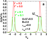
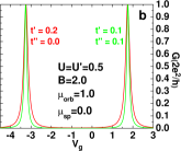
Figure 3: Illustration of the difference between SU(4) and 2LSU(2) Kondo states. (a) By applying an external magnetic field and making $\mu_{orb}=0.0$ and $\mu_{sp}B=2.0$, one suppresses the spin Kondo effect. In this case, the SU(4) Kondo peak seen in Fig. 2 (red curve) splits into two orbital SU(2) Kondo peaks (red curve), where the degree of freedom being screened is the orbital one. However, in the case of the 2LSU(2) (green curve), as the spin Kondo effect has been suppressed by the field and since there is no orbital Kondo effect in the 2LSU(2) state, one can see the two sets of CB peaks separated by $U^{\prime}$ (green curve). (b) On the other hand, when $\mu_{orb}B=2.0$ and $\mu_{sp}=0.0$, one is left with a spin SU(2) Kondo effect for each orbital level in both states (SU(4) and 2LSU(2)), as is clearly shown by the two Kondo peaks separated by a distance proportional to the applied field.

IV Comparison of SU(4) with 2LSU(2) and transition between both states

To illustrate the entanglement of the charge and spin degrees of freedom in the SU(4) state, we compare results for $t^{\prime\prime}=0$ and $t^{\prime\prime}=t^{\prime}$, i.e., for the SU(4) and 2LSU(2) states (see Fig. 1), respectively. In Figs. 3a and 3b it is shown a comparison between them when a magnetic field acts only on the spin degree of freedom (Fig. 3a) or only on the orbital degree of freedom (3b). By making $\mu_{orb}=0.0$ and $\mu_{sp}B=2.0$ (3a), the spin Kondo effect is suppressed, since the spin levels are split by an energy larger than the Kondo temperature, while the orbital levels are unaffected. Therefore, the SU(4) Kondo peak splits into two orbital SU(2) Kondo peaks separated by a distance proportional to the field (red curve) lipinski . On the other hand, since in the 2LSU(2) state there is no orbital Kondo effect (since the orbital quantum number is not conserved upon tunneling), by suppressing the spin Kondo with the magnetic field one is left with just two sets of Coulomb Blockade (CB) peaks (split by $U^{\prime}$) separated by a splitting proportional to the field (green curve). In contrast, when only the orbital levels are split by the magnetic field ($\mu_{orb}B=2.0$ and $\mu_{sp}=0.0$), one is left with two spin SU(2) Kondo peaks (one for each orbital level) for both states, as can be seen in Fig. 3b.

At zero field, it is then not really surprising that the SU(4) state depicted by the red curve in Fig. 2a will change once the channels are allowed to ‘talk’ to each other (finite $t^{\prime\prime}$, see green arrows in Fig. 1), i. e., if an electron that tunnels into the CNT QD through one channel has a finite probability of tunneling out through the other channel. Figure 4 shows results comparing the SU(4) state ($t^{\prime}=0.2$, $t^{\prime\prime}=0.0$) with the 2LSU(2) state ($t^{\prime}=t^{\prime\prime}=0.1$) note2 . Notice that the conductances for the two states, although being both equal to $2e^{2}/h$ at QF friedel , are qualitatively very different: the 2LSU(2) state reaches a maximum of $2e^{2}/h$, half of the maximum in the SU(4) state, and it resembles more the results for a single-channel system discontinuity .

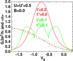
Figure 4: Comparing SU(4) and 2LSU(2) conductances: The red curves show the conductance $G$ (solid) and average occupancy $\left<n\right>$ (dashed) for the SU(4) state (same as the red curves in Fig. 2), while the green curves show results for 2LSU(2). It is interesting to note that for both states, when the CNT is occupied by one electron ($V_{g}=-0.25$ for 2LSU(2), and $V_{g}=-0.385$ for SU(4)), the conductance reaches the unitary limit ($G=2e^{2}/h$), as discussed in ref. aguado1, , however there is no question that the conductances for both states are qualitatively different.

It is reasonable to assume that in a realistic experimental situation the conservation of the orbital quantum number lies somewhere between the two schemes represented in fig. 1, therefore a careful analysis of the robustness of the SU(4) state (in the presence of some channel mixing) is needed if one wants to correlate any of the experimental observations to the results obtained by numerical modeling. Recent calculations aguado1 ; aguado2 have analyzed the transition between these two states (SU(4) and 2LSU(2)) only at QF. In figure 5, we present complementary calculations for all fillings. Our results at QF confirm (as discussed below) that SU(4) and 2LSU(2) at QF are experimentally indistinguishable, reinforcing then the need to extend the analysis to other fillings, especially between QF and HF.

Figure 5 shows how the conductance evolves from the SU(4) to the 2LSU(2) state, for $t^{\prime\prime}$ varying from $0$ to $t^{\prime}$. Notice that, as the value of $t^{\prime\prime}$ increases from zero (solid black curve), the conductance peak at $4e^{2}/h$ (characteristic of the SU(4) state) becomes gradually narrower, until (for $t^{\prime\prime}>0.175$) the central peak splits into three very narrow peaks (not shown). An indication of their presence can be seen already in the curve for $t^{\prime\prime}=0.175$ (cyan), as indicated by the arrows. As $t^{\prime\prime}$ approaches $t^{\prime}$, these three peaks continue to narrow, until they vanish. On the other hand, for values of conductance around $2e^{2}/h$, the curve develops shoulders which become broader as $t^{\prime\prime}$ increases. We want to stress the qualitative agreement of our QF results to those obtained by J.-S. Lim et al. aguado2 . In fig. 5, all curves cross at $V_{g}\approx-0.3$ (where $\langle n_{d}\rangle\approx 1$, QF) where they have approximately unitary conductance $G_{0}$. Therefore, as stressed in references aguado1, and aguado2, , SU(4) and 2LSU(2) are experimentally indistinguishable at QF and zero magnetic field. In addition, it is also interesting to note, as described above, that our results for $t^{\prime\prime}\approx t^{\prime}$ change discontinuously to the 2LSU(2) result (dashed curve). A similar discontinuity is seen in the Slave Boson Mean Field results at QF in reference aguado2, (please, check their fig. 14).

Finally, the green solid curve in fig. 4 has a discontinuity in the conductance for $V_{g}=-0.5$. We have seen this kind of behavior in other multi-orbital systems discontinuity , and in some cases associated it to the crossing through the Fermi energy of a very narrow level. This causes an abrupt charging of the QD (clearly visible in the green dashed curve for $\langle n_{d}\rangle$ vs. $V_{g}$), with the consequent abrupt change of the conductance. In this specific case, this level can be identified to the $\epsilon_{-}$ energy level in the upper panel of fig. 11 in reference aguado2, , which, as described there, has a vanishingly narrow width.

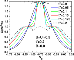
Figure 5: Transition from the SU(4) to the 2LSU(2) state: Results showing the variation of the conductance for $t^{\prime\prime}$ varying from 0.0 (black curve) to 0.2 (dashed), going through the values 0.05 (blue), 0.1 (green), 0.15 (red) and 0.175 (cyan). $U=U^{\prime}=0.5$ and $t^{\prime}=0.2$.

V Experimental observation of SU(4) Kondo at Half-Filling

Figure 6a reproduces Fig. SI2 in the Supplementary Information of ref. jarillo, . In it, the temperature variation of the conductance for three shells in the CNT QD is reported (thick red line at higher temperature and black thin line for the lowest temperature). Notice that the coupling to the leads increases from right to left jarillo ; jarillo2 (that is why the conductance of shell 1 is the lowest). In reference jarillo, , the conductance in regions I and III in the second shell was associated to a QF SU(4) state and the conductance at HF in shell $n=3$ was associated to a singlet-triplet effect sasaki ; yeyati . However, in Fig. 6b, our results indicate an alternative interpretation: by breaking the degeneracy of the orbital levels (by introducing a small energy splitting $\delta E=0.032$) splitting and by increasing the coupling of the third shell to the leads ($t^{\prime}=0.2$) in relation to the second shell ($t^{\prime}=0.11$), the experimental results can be qualitatively reproduced. Note that since our calculations are done at zero-temperature, the curve in Fig. 6b should be compared to the highest conductance curve in Fig. 6a (thin black line). It is clear that the qualitative agreement is quite good.

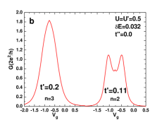
Figure 6: (a) Adapted from Supplementary Information in ref. jarillo, (Fig. SI2): temperature dependence of the conductance for the three shells observed in the CNT QD. Thick red curve at higher temperature and thin black curve at lowest temperature. Note that the coupling to the leads increases from right to left (from shell $n=1$ to $n=3$) jarillo ; jarillo2 . In ref. jarillo, , the regions indicated as I and III in the second shell were interpreted as indicative of the presence of a QF SU(4) state and the conductance of the third shell (leftmost) was associated to a singlet-triplet state sasaki , however, our simulations in (b) show that the conductance for both shells can be interpreted as indication of a QF SU(4) state for the second shell and of both QF and HF SU(4) states for the third shell. These results are obtained by adding a small energy separation between the orbital levels ($\delta E=0.032$) and by increasing the coupling of the third shell ($t^{\prime}=0.2$) in relation to the second shell ($t^{\prime}=0.11$).

To further test our simulations against the experimental results, Fig. 7a shows a color-scale plot with numerical results for the variation of the conductance (at zero bias) with applied magnetic field (along the CNT axis) for the third shell (same parameters as the ones used in Fig. 6b). Since the orbital moment is much larger than the spin one ($\mu_{orb}=0.2$ and $\mu_{sp}=0.04$), at lower fields one sees first the splitting of the SU(4) conductance peak into two spin SU(2) Kondo peaks, which at higher field values will each further split into two CB peaks. Figure 7b shows a figure adapted from ref. jarillo2, containing field-dependent conductance results (third shell in Fig. 6a) which are clearly in qualitative agreement with the numerical results in Fig. 7a. The combined results presented in Figs. 6 and 7 present compelling evidence that the conductance results of the third shell can be interpreted as a manifestation of the HF SU(4) state. It is interesting to note the asymmetry in the conductance in the experimental results in Fig. 7b, i.e., the CB regime is reached at lower values of field for lower values of gate voltage. The same kind of asymmetry was observed by Makarovski et al. gleb in all shells and always with the higher conductance for 3 electrons in the shell. It is not clear yet the reason for this higher Kondo temperature for 3 electrons when compared to QF (1 electron inside the shell).

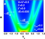
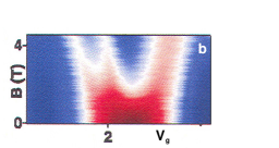
Figure 7: Splitting of the Kondo SU(4) peak caused by an external magnetic field applied along the CNT axis. (a) Color-scale plot of the conductance showing the progressive splitting of the zero-field SU(4) peak into two spin SU(2) peaks and then into 4 CB peaks (dark red $\approx 4e^{2}/h$ and blue $=0$). (b) Experimental results adapted from ref. jarillo2, (same shell as the leftmost one in Fig. 6a) indicating that the numerical results in part (a) qualitatively reproduce the experiments.

VI Conclusions

In summary, using a recently developed numerical method (ECA) method , the authors offer a reinterpretation of recent transport measurements in CNT QDs. In these experiments, the conductance of one of the electronic shells of a CNT QD was associated to the SU(4) Kondo effect at QF, and the conductance at HF of an adjacent shell was interpreted as resulting from a singlet-triplet effect jarillo . Our results clearly show that the conductance of both shells can be interpreted instead as resulting from an SU(4) statenote-st : this is achieved by introducing a small energy splitting between the orbital levels and increasing the coupling to the leads of one of the shells in relation to the other (see Fig. 6). Furthermore, simulations of conductance at finite magnetic field give support to our interpretation. These results open the possibility that the SU(4) state at HF could be analyzed in detail in CNT QDs. The fact that recent NRG results by Galpin et al. galpin1 have associated this state to rich physical behavior, including a non-Fermi-liquid phase, adds to the importance of our results. In addition, simulations presented in Fig. 2 are in qualitative agreement with Galpin et al.’s NRG results. This suggests that the low-energy physics associated to their NRG results is quite robust and should in principle be observed experimentally.

One last point the authors would like to stress is related to the implications of the SU(4) ‘spin-orbital entanglement’ to the structure of the Kondo cloud. A qualitative description of the screening mechanism in the Kondo effect involves the existence of the so-called ‘Kondo cloud’: associated to the Kondo temperature $T_{K}$ (a universal energy scale which emerges naturally from Renormalization Group arguments) there is a universal length scale $\xi_{K}=\hbar v_{F}/T_{K}$, which can be interpreted as the size of the many-body wave function containing the conduction electron that forms a singlet with the impurity spin. Even before the first measurement of the Kondo effect in semiconducting QDs goldhaber2 , there was great interest in experimentally detecting the Kondo cloud, with theoretical bergmann and experimental giordano efforts being made to evaluate and measure its size and dependence on dimensionality. The failure to actually observe the extent of the Kondo cloud (or even ascertain its existence) underscores the difficulties involved. This has lead more recently to theoretical efforts to analyze setups where the Fermi sea is effectively ‘confined’ inside the nanostructure, like for example in the so-called ‘Kondo Box’ thimm or in QDs embedded in Aharonov-Bohm (AB) rings affleck . In such setups, interesting new effects are expected to occur, hopefully leading to a better understanding of the screening effect and a possible direct or indirect breakthrough measurement of the Kondo cloud. The difficulty of fabricating the proposed devices and performing the necessary measurements may explain the fact that most of the work in this area is theoretical. Referring back to fig. 1, the many-body wave function formed by conduction electrons that screen the localized moment has to have quite different properties in the SU(4) Kondo state when compared to the 2LSU(2) state. Indeed, the recognition that orbital Kondo correlations can only form if the orbital QN is conserved upon tunneling, and that electron states in the metallic leads do not have a defined ‘wrapping mode’, results in the natural conclusion that in the SU(4) Kondo state the ‘Fermi sea’ is in reality formed by electrons that have a well defined orbital QN, and therefore should reside primarily in the regions of the CNT contained between the tunnel barrier and the metallic contacts jarillo ; aguado1 ; aguado2 . These regions, as for example in the proposed setups involving QDs embedded in AB rings affleck , naturally constrain the extent of the Kondo cloud. Obviously, for CNT devices where the tunneling barrier is exactly at the interface between the CNT and the metallic contacts, there is no conservation of the orbital QN, leading to a 2LSU(2) state, where there is no entanglement of the spin and orbital degrees of freedom and therefore its associated Kondo cloud is free to spread inside the metallic contacts. One of the problems with the experimental realization of setups suggested as possible probes of the Kondo cloud properties is that, once leads are attached to the nanostructure to perform actual measurements, the Kondo cloud spreads into them, making the measurements of its properties difficult. What we suggest here is that the SU(4) state in carbon nanotubes naturally provides a system where the Kondo cloud should be constrained inside the nanostructure itself, with the advantage that the leads needed for conductance measurements, at least in principle, do not ‘accept’ the Kondo cloud. In that case, careful analysis of the change in transport properties as the system transitions from the SU(4) to the 2LSU(2) state should provide valuable information about the screening process and at least some indirect information about the Kondo cloud.

The authors acknowledge useful discussions with E. Anda, E. Dagotto, G. Finkelstein, D. Goldhaber-Gordon, P. Jarillo-Herrero and J. Riera. G. B. M. acknowledges support from Research Corporation; C. A. B. acknowledges support from UT, Knoxville.

References

- (1) P. Jarillo-Herrero et al., Nature 434, 484 (2005).
- (2) U. Wilhelm et al., Physica E 14, 385 (2002).
- (3) A. W. Holleitner et al., Phys. Rev. B 70, 075204 (2004).
- (4) S. Sasaki et al., Phys. Rev. Lett. 93, 017205 (2004).
- (5) T. Pohjola et al., Europh. Lett. 54, 241 (2001).
- (6) L. Borda et al., Phys. Rev. Lett. 90, 026602 (2003).
- (7) G. Zarand, Philos. Mag. 86, 2043 (2006).
- (8) P.G. Silvestrov and Y. Imry, cond-mat/0609355 (2006) and K. Le Hur et al., cond-mat/0609298 (2006).
- (9) A. Makarovski et al., cond-mat/0608573.
- (10) The Kondo temperature observed in the orbitally degenerate CNT QD was as high as jarillo .
- (11) M. Iroi et al., Phys. Rev. B 55, 8339 (1997).
- (12) R. C. Toonen et al., cond-mat/0512235 (2005).
- (13) R. M. Potok and D. Goldhaber-Gordon, Nature 434, 451 (2005).
- (14) M.-S. Choi et al., Phys. Rev. Lett. 95, 067204 (2005).
- (15) J.-S. Lim et al., cond-mat/0608110. In this manuscript, Renormalization Group, Numerical Renormalization Group, Slave Boson Mean Field, and Non Crossing Approximation where employed to analyze the transport properties of CNT QDs.
- (16) M. R. Galpin et al., Phys. Rev. Lett. 94, 186406 (2005), where the properties of a Quantum Critical Point at HF were studied. The fact that the model for a double-orbital QD coupled to double channel leads displays a Kondo effect with entanglement of spin and charge degrees of freedom not only at QF, but also at HF, has been mostly overlooked in the analysis of experimental results jarillo ; aguado1 .
- (17) M. R. Galpin et al., cond-mat/0608169 and cond-mat/0608186.
- (18) V. Ferrari et al. Phys. Rev. Lett. 82, 5088 (1999)
- (19) S. Sasaki et al., Nature 405, 764 (2000).
- (20) P. Jarillo-Herrero et al., Phys. Rev. Lett. 94, 156802 (2005).
- (21) E. D. Minot et. al, Nature 428, 536 (2004).
- (22) For a discussion about the origin and properties of these two channels in the devices used in the experiments, please see last paragraph in ref. jarillo, .
- (23) Y. Meir et al., Phys. Rev. Lett. 66, 3048 (1991).
- (24) M. R. Buitelaar et al., Phys. Rev. Lett. 88, 156801 (2002).
- (25) As noted in reference galpin1, , one expects that the SU(4) state on each side of the point will survive for an interval .
- (26) A similar effect, taking advantage of the existence of an SU(4) state in double-QDs (where ), is suggested by S. Lipinski and D. Krychowski (cond-mat/0512726 (2005)) as a way to perform spin filtering of the transmitted electrons.
- (27) A smaller value is used for the hoppings in the 2LSU(2) state to compensate for the fact that the number of hoppings between the QD and the leads in 2LSU(2) is double that in SU(4) (see Fig. 1).
- (28) This can be obtained in a very simple way by invoking the Friedel sum rule (check reference aguado1, ).
- (29) Single-channel results for multi-orbital systems obtained with the ECA method were reported in C. A. Busser et al., Phys. Rev. B 70, 245303 (2004) for 1 QD, and in G. B. Martins et al., Phys. Rev. Lett. 94, 026804 (2005) for 2 QDs. The discontinuities seen in and for the 2LSU(2) state (green curves) have also been obtained in similar systems by applying a variety of different techniques (see, for example, P. G. Silvestrov and Y. Imry, Phys. Rev. B 65, 035309 (2001) and M. Sindel et al., Phys. Rev. B 72, 125316 (2005)).
- (30) Notice that the temperature variation obtained for the SU(4) HF effect (A. L. Yeyati et al., Phys. Rev. Lett. 83, 600 (1999)) describes the data for the third shell better than the singlet-triplet effect (W. Izumida et. al, Phys. Rev. Lett. 87, 216803 (2001)).
- (31) This claim can be tested by measuring the variation of away from the orbital degeneracy point: it should be asymmetric for ST and symmetric for SU(4), as indicated in reference sasaki1, .
- (32) D. Goldhaber-Gordon et al., Nature 391, 156 (1998).
- (33) G. Bergmann, Phys. Rev. Lett. 67, 2545 (1991).
- (34) M. A. Blachly and N. Girodano, Phys. Rev. B 51, 12537 (1995).
- (35) W. B. Thimm et al., Phys. Rev. Lett. 82, 2143 (1999).
- (36) I. Affleck and P. Simon, Phys. Rev. Lett. 86, 2854 (2001).