Stiff knots

Abstract

We report on the geometry and mechanics of knotted stiff strings. We discuss both closed and open knots. Our two main results are: (i) Their equilibrium energy as well as the equilibrium tension for open knots depend on the type of knot as the square of the bridge number; (ii) Braid localization is found to be a general feature of stiff strings entanglements, while angles and knot localization are forbidden. Moreover, we identify a family of knots for which the equilibrium shape is a circular braid. Two other equilibrium shapes are found from Monte Carlo simulations. These three shapes are confirmed by rudimentary experiments. Our approach is also extended to the problem of the minimization of the length of a knotted string with a maximum allowed curvature.

I Introduction

We report on the properties of stiff knots, i.e. knotted strings whose shape is dictated by the bending curvature energy and contact interactions only. Stiff knots, such as loose knots with nylon or metal strings, are ordinary objects in everyday life (Fig.1). An upsurge of interest in stiff knots recently came from studies which pertain to microscopic objects, such as those encountered in biology and nano-technologies. Some examples are: knots with actin filaments actin , nanotubes Lobovkina2004 , nanotube fibers macro , and silica wires Tong2003 (see Fig. 1). These studies point out the relevance of stiff knots for the experimental determination of the bending rigidity actin , for knot induced polymer and filament break-up Saitta1999 ; actin , and for nano-manipulation Lobovkina2004 .

Moreover, many recent experimental and theoretical studies were devoted to knots in polymers, with an emphasis on knotted DNA Quake_Vilgis_Katrich . They show that flexible polymers are subject to knot localisation leading to the formation of small prime knots. Knot localization may result from entropic effects knot_loc_entro , or long range interactions knot_loc_inter ; O'Hara2003 . If the localized knots are small enough, their thermal fluctuations become negligible and they might be described by the stiff knot regime.

Finally, stiff knots may be considered as elementary entanglements which capture qualitatively some of the features of more complex entanglements. Hence, stiff knots may also provide insights for the curvature energy dominated behavior of tightly entangled semi-flexible polymers such as actinactin-solutions ; Morse2001 , and other fibrous materials Rodney2005 .

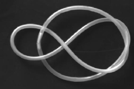
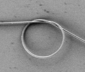
Figure 1: Stiff knots. Upper panel: A closed knot, made with a plastic tube of width $1$ cm and length $80$ cm (see section IX.3 for details). Lower panel: Open trefoil knot with a silica nanowire, from Ref.Tong2003 . The width of the picture is 20 $\mu$m.

Here, we aim to establish the basic mechanical and geometrical properties of stiff knots. First, the mechanical properties of the knots are found to exhibit a surprisingly simple dependence on the knot type via a quantity called the bridge number $n$ (to be defined below). We show that the minimum knot energy, as well as the minimum equilibrium tension at the open ends of an open knot, both increase with $n$ as $n^{2}$. Secondly, we identify a striking and general feature of the geometry of stiff strings entanglements, which we call braid localization. We analyze the geometries of the simplest knots which indeed exhibit braid localization.

We will begin with a study of closed knots. In section II, we define the curvature energy of a filament. In section III, we discuss the role of interactions on the equilibrium shape of a filament, and we place our problem within the historical perspective of the studies on the so-called Bernoulli-Euler elastica. A lower bound for the energy of the equilibrium configuration is given in section IV. In section V, we analyze the limit of thin strings which leads to braid localization. In section VI, the results of section V are used in order to obtain upper bounds for the equilibrium energy. Two results follow from the existence of these upper bounds: (i) the global minimum of the energy scales as $n^{2}$; (ii) the minimization problem is solved exactly for a special family of knots. The shape and energy of some simple knots are obtained from Monte Carlo Simulations in section VII. We find three geometries which correspond to the simplest knots. In section VIII, we translate the main results of our analysis to the case of open knots. In section IX, we discuss several additional points: (i) the equivalence between the limits of thin strings and long strings; (ii) the curvature energy of thick knots; (iii) rudimentary experiments; (iv) the restricted curvature model, which makes link with the work of Buck and Rawdon Buck2004 . Finally, we conclude in section X.

II Model

We shall first focus on closed knots, i.e. single knotted strings without free end, as in the upper panel of Fig.1. A given configuration of a knot in 3D space is described by a position vector ${\bf r}(s)$, where $s$ is the arclength. Since the knot is closed, ${\bf r}(s)$ is periodic in $s$, and its period is the length

$${\cal L}=\int ds,$$ (1)

of the knot. In the following, the absence of bounds in the integrals indicates integration over the whole knot. We define the usual curvature energy of an inextensible stringDoi ; kamien as:

$${\cal E}={C\over 2}\int ds\,\kappa^{2},$$ (2)

where $\kappa\geq 0$ is the curvature, and $C$ is the bending rigidity. Such a modelling is valid in the limit of small deformations, defined by the limit of small curvature Doi :

$$w\kappa\ll 1$$ (3)

where $w$ is the diameter of the section of the filament.

The question we address is the following: for a given knot $K$ of length ${\cal L}$, what are the equilibrium shape and energy? We call equilibrium energy the global minimum energy, as opposed to that corresponding to possible other local minima, which will be referred to as metastable states. The equilibrium energy is denoted as ${\cal E}^{*}$. We shall fix ${\cal L}$ by means of a Lagrange multiplier $\mu$. Mechanical equilibrium is then obtained from the minimization of:

$${\cal F}={\cal E}+\mu{\cal L}={C\over 2}\int ds\,\kappa^{2}+\mu\int ds\,.$$ (4)

III On the role of interactions

Let us first consider this minimization problem in the absence of interactions between the different parts of the strings. In this case, the curve can freely cross itself. We obtain the so-called elastica, initially proposed by D. Bernoulli. In order to investigate further this problem, we consider the variation of ${\cal F}$ induced by the variation $\delta{\bf r}(s)$ of the position of the string. Since the filament is closed, there is no boundary terms and:

$$\delta{\cal F}=\int ds\;\delta{\bf r}.\partial_{s}{\bf A}$$ (5)

where

$${\bf A}=\left({C\over 2}\kappa^{2}-\mu\right){\bf t}+C\partial_{s}\kappa\,{\bf n}+C\kappa\tau\,{\bf b}\,.$$ (6)

Throughout the paper, we denote the derivatives with respect to $s$ as $\partial_{s}$. At equilibrium, the energy variation vanishes: $\delta{\cal F}=0$, leading to the nonlinear differential system $\partial_{s}{\bf A}=0$, i.e. ${\bf A}$ is constant, andDoi

$${C\over 2}\kappa^{2}-\mu = {\bf A.t}\,,$$ (7)

$$-C\kappa\tau = {\bf A.b}\,.$$ (8)

The constant vector ${\bf A}$ represents the internal forces in the string Doi , $\tau$ is the torsion, ${\bf t}=\partial_{s}{\bf r}$ is the tangent vector of the curve, and $({\bf t,n,b})$ is the usual Frenet frame. We have not written down the projection of ${\bf A}$ on ${\bf n}$ because it is redundant. Indeed, it and can be obtained from a derivation of (7) with respect to $s$.

But $\delta{\cal F}$ does not vanish only at the global minimum (i.e. at equilibrium), and a number of other spurious solutions are found. Planar solutions of (7,8) were analyzed by Euler Euler . The 3D solutions are listed in Ref.Langer, . Comparing their energies, one finds that the circle is the closed solution with the lowest energy. It is also the only closed solution which is stable Langer . Thus, knots cannot be stable solutions of (7,8). Knots can nevertheless be stabilized in the presence of interactions between the different parts of the string.

In the following, we use a hard core repulsion, and the string is modelled by means of a non-self-intersecting tube of diameter $w$. Such a hard core repulsion implies that the distance between different parts of the string is larger than $w$, and the radius of curvature $1/\kappa$ is larger than $w/2$ (see e.g. Ref. O'Hara2003, ). In the previous paragraph, we concluded that knots could not be stabilized in the absence of interactions. In the case of hard core repulsion, such a statement means that contact points must be present.

But the non-crossing condition at contact points involves interactions between distant parts of the string (i.e. parts with different values of $s$). These interactions can be included in the energy (2) by means of an additional term which includes a nonlocal interaction potential. In the variational formulation, such a term leads to additional nonlinear integro-differential contributions to (7,8), the consequences of which are difficult to analyze. Despite the difficulty, some mathematical informations about the solutions – such as their existence– were obtained from this approach vonderMosel1998 .

We here consider a different approach based on a combined analysis of the knot topology and of the geometry in the limit of vanishing string width $w\rightarrow 0$. Our approach does not systematically provide the equilibrium configuration and its energy, but it allows one to obtain important information about the equilibrium energy (such as lower and upper bounds), and about the geometry of the equilibrium configuration (such as the absence of knot localization and the presence of braid localization).

IV Lower bound for the energy

We start with a result found by J.W. Milnor Milnor1950 : for any given knot $K$,

$$2\pi n\leq\bar{\kappa}\,,$$ (9)

where

$$\bar{\kappa}=\int ds\kappa$$ (10)

is a dimensionless quantity called the total curvatureO'Hara2003 , and $n$ is the bridge number of the knot $K$. To define $n$, let us consider a given direction in space $\hat{\bf x}$. As shown in Fig. 2, any given configuration ${\bf r}(s)$ of $K$ in space has a well defined number of maxima along $\hat{\bf x}$. The minimum number of maxima among all configurations of $K$ is $n$. Deforming the knot so as to place all maxima and all minima in two parallel planes of fixed abscissa along $\hat{\bf x}$, we obtain the linear braid configuration of figure 3b. The minimum number of loops at the top of the braid is $n$. For an unknotted closed string (usually called the unknot), $n=1$, and for any other knot $n\geq 2$. For example, $n=2$ for most DNA knots Wasserman1986 .

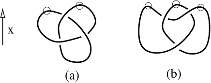
Figure 2: The trefoil knot can be represented in different ways in 3D space such as in (a) and (b). For each configuration, there is a given number of maxima along the $x$ axis: 2 in (a), and 3 in (b). The minimum number of maxima among all configurations of the knot is the bridge number $n$. On the figure, we have drawn the trefoil knot, for which $n=2$.

We define the normalized energy

$$\epsilon={{\cal E}{\cal L}\over C}$$ (11)

which depends on the knot shape, but is independent of the knot size and bending rigidity. Hence, $\epsilon$ only depends on $w/{\cal L}$ and on the type of knot. Using the Schwarz inequality:

$$\left(\int ds\,\kappa^{2}\right)\left(\int ds\right)\geq\left(\int ds\,\kappa\right)^{2}=\bar{\kappa}^{2}$$ (12)

and (9), we find:

$$2\pi^{2}n^{2}\leq{\bar{\kappa}}^{2}/2\leq\epsilon\,.$$ (13)

This generalizes a result of Ref.kamien, , which reads in our notations: $\epsilon\geq 8\pi^{2}$, and which can be obtained from (13) with the additional knotting condition $n\geq 2$.

Figure 3: Knots in ordinary 3D space. Any knot (a) can be deformed to a braid and loop configuration (b) with $n$ maxima, or to a closed braid configuration (c) with $i$ strands (here $n=2$ and $i=3$). The lateral shrinking of (b) leads to the configuration (d) with the lowest total curvature $\bar{\kappa}=2\pi n$. When the central braid of (b) is shrinked to a point, and the loops are solutions of Eqs.(7,8), we obtain the Point Braid and Loops configuration (e). In (f), the closed braid is laterally shrinked, and has a circular shape.

Note that (9) is sharp: for any knot, it becomes an equality for the laterally shrinked configuration of Fig.2d. Nevertheless, (13) is not necessarily sharp: it only provides a lower bound for the energy. Since it is a lower bound for all configurations, it is also a lower bound for the equilibrium energy. This lower bound depends on the knot type via $n$ and but does not depend on the filament width $w$.

V Asymptotics of thin strings and braid localization

V.1 Variation of the energy with $w$

The energy ${\cal E}^{*}_{w}$ of the equilibrium configuration of a knot $K$ is a monotonically increasing function of $w$. The proof of this statement is reported in Appendix A. We may therefore write:

$$\partial_{w}{\cal E}^{*}_{w}\geq 0$$ (14)

Hence, if we consider the equilibrium shapes ${\cal E}^{*}_{w}$ of a given knot $K$ as a function of $w$, the lowest value of ${\cal E}^{*}_{w}$ will be reached in the limit $w\rightarrow 0$. On the opposite, the highest value of ${\cal E}^{*}_{w}$ will be reached by the tight knotDegennes , also called ideal knotStaziak , which is the configuration with the highest possible value $w_{id}$ of $w$ authorized by the hard core repulsion. This can be summarized as:

$${\cal E}^{*}\leq{\cal E}^{*}_{w}\leq{\cal E}^{*}_{w_{id}}.$$ (15)

where ${\cal E}^{*}=\lim_{w\rightarrow 0}{\cal E}^{*}_{w}$.

Here, we will not analyze the full dependence of ${\cal E}^{*}_{w}$ with respect to $w$, but we rather focus of the limit $w\rightarrow 0$. The reason of our focus on this limit is self-consistency. Indeed, the expression of the energy ${\cal E}$, defined in Eq.(2), is valid in the limit (3). Integrating (3) along the knot, we find $w\bar{\kappa}\ll{\cal L}$. Then, using (9), we obtain

$${w\over{\cal L}}\ll{1\over 2\pi n}\,.$$ (16)

Since we consider a given knot (i.e. fixed $n$) with a fixed length (i.e. fixed ${\cal L}$), the limit $w\rightarrow 0$ is required for the energy ${\cal E}_{w}$ of a knot to be well-defined.

V.2 Configurations in the limit $w\rightarrow 0$

We now analyze the knot configurations in the limit $w\rightarrow 0$. They are obtained from a procedure in 2 steps. (i) Identification a possible structure $\{{\cal S}\}$ of the knot when $w\rightarrow 0$. (ii) Variational approach on the structure $\{{\cal S}\}$.

V.2.1 Structure

In step (i), we take the limit $w\rightarrow 0$ which may lead to “wild knots”, exhibiting knot accumulations or singularities. We shall determine which types of accumulations or singularities are allowed, and which ones are forbidden.

The 4 possible types of singularities or accumulations are given on Fig.4. Angular points –as in Fig.4a, and knot localization –as in Fig.4b, are forbidden because they lead to an infinite energy. A rigorous proof of this statement is given in Appendix B. Here, we only provide an intuitive explanation: angles and knot localization may be obtained by decreasing the length ${\cal L}_{loc}$ of a part of a curve to zero, keeping its shape fixed. An example of such a shrinkage is shown on Fig. 4, where the size of the dashed box containing the angle decreases. Using Eq.(11), the energy of this part behaves as ${\cal E}_{loc}=C\epsilon/{\cal L}_{loc}$ where $\epsilon$ depends on the shape but not on the scale. Since ${\cal L}_{loc}\rightarrow 0$, one has ${\cal E}_{loc}\rightarrow\infty$.

Figure 4: In the limit where the string width $w$ vanishes, various singularities or accumulations may occur. The thickness of the lines are used to represent various filament widths $w$. (a) angle. The dashed line defines a box whose size is shrinked to zero to obtain localization. The filament length in the box is ${\cal L}_{loc}$. see text; (b) knot localization; (c) multiple point; (d) braid localization, leading to a line-braid, or a point braid. Angles and knot localization are forbidden because they lead to divergence of the energy ${\cal E}$.

The two types of accumulations which are allowed when $w\rightarrow 0$ are multiple points –as in Fig. 4c, or braid localization –as in Fig.4d, because they do not lead to a divergence of ${\cal E}$.

Braid localization is defined as the lateral shrinking of a braid, with all strings in the braid tending to the same curve. We define a line-braid of multiplicity $m\geq 1$ as the result of the lateral shrinking of a braid of $m$ strings. In the following, a single string will be considered as a line-braid with multiplicity $m=1$. Since all strings in the braid tend to the same curve, the curvature energy of the line-braid reads $mC/2\int ds\,\kappa^{2}$.

In some cases, we might then also shrink the length of the braid to zero to obtain a point-braid, as in Fig. 4d. The order of the limits is important: firstly lateral shrinking, and secondly length shrinking, so that the curvature energy of the point-braid vanishes. Since angle localization is forbidden, strings or line-braids must emerge tangentially along the same axis from a point-braid.

By shrinking braids in a special way with a given knot, we obtain a structure $\{{\cal S}\}$ of line-braids connected by multiple points or point-braids. An example of such a structure is depicted on Fig.5.

At this point, we shall put some emphasis on a central result of the present section: in the limit $w\rightarrow 0$, knot localization is forbidden and braid localization is expected. We shall also stress on the fact that we have not proved that braid localization will occur, but we have shown that it can occur when $w\rightarrow 0$.

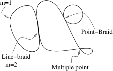
Figure 5: Shape of a knot in the limit $w\rightarrow 0$: an ensemble of line-braids connected by multiple points or point-braids. The drawing is 2D but we consider 3D configurations throughout the manuscript.

V.2.2 Variational analysis of a structure

In this section, we derive the conditions which must be satisfied at equilibrium from a variational approach. We consider a given structure $\{{\cal S}\}$, with $N$ line-braids. Its energy reads:

$${\cal E}_{\{{\cal S}\}}=\sum_{p=1}^{N}{m_{p}C\over 2}\int_{p}ds\kappa^{2}$$ (17)

where the index $p$ in the integral means that the integration is performed over the $p$th line-braid only, and $m_{p}$ is the multiplicity of the $p$th line-braid. As in section II, the total length is fixed by means of a Lagrange multiplier $\mu$, and we have to minimize:

$${\cal F}_{\{{\cal S}\}}=\sum_{p=1}^{N}\left[{m_{p}C\over 2}\int_{p}ds\kappa^{2}+\mu m_{p}\int_{p}ds\right]$$ (18)

The variation of ${\cal F}_{\{{\cal S}\}}$ resulting from a variation $\delta{\bf r}(s)$ of the structure $\{{\cal S}\}$ reads:

$$\delta{\cal F}_{\{{\cal S}\}}=\sum_{p=1}^{N} \left\{\int_{p}ds\;\delta{\bf r}.\partial_{s}{\bf A}_{p}\right.$$ (19)

$$+\left.\left[-\delta{\bf r}.{\bf A}_{p}+Cm_{p}\kappa\,{\bf n}.\partial_{s}\delta{\bf r}\right]_{p}\right\}$$

where $[Y]_{p}$ indicates the difference between $Y$ at the end of the $p$th line braid, and $Y$ at its beginning. Moreover,

$${\bf A}_{p}=m_{p}\left[\left({C\over 2}\kappa^{2}-\mu\right){\bf t}+C\partial_{s}\kappa\,{\bf n}+C\kappa\tau\,{\bf b}\right]\,.$$ (20)

At equilibrium, one has $\delta{\cal F}=0$, which leads to $\partial_{s}{\bf A}_{p}=0$, so that ${\bf A}_{p}$ is a constant vector. Projecting ${\bf A}_{p}$ on ${\bf t}$ and ${\bf b}$, we find:

$$m_{p}\left[{C\over 2}\kappa^{2}-\mu\right] = {\bf A}_{p}.{\bf t}\,,$$ (21)

$$-m_{p}C\kappa\tau = {\bf A}_{p}.{\bf b}\,.$$ (22)

At equilibrium, line-braids therefore obey differential equations similar to that of single strings (7-8).

Let us now discuss the boundary conditions at the contact points (multiple points or point-braids) between the line-braids. We use the index $B$ to list the points at which the line-braids are connected. At a point $B$, several strings related to different line-braids and point-braids may cross. Two types of constraints may force the strings which cross at $B$ to be tangent to each other. (i) Since angle localization is forbidden, each string enters and exits at the point $B$ with the same tangent vector. (ii) Each string is also tangent to some other strings because it belongs to a line-braid or a point-braid. The combination of these two constraints forces a bunch of line-braids ending at $B$ to be tangent to each other at the contact point. There might be several bunches of line-braids at the point $B$. These bunches can rotate freely from each other, but all braids inside the bunch are tangent to each other at the point $B$. Let $q_{B}$ be the index which lists the bunches at the point $B$. The boundary contribution of the variation (19) may then be re-written as:

$$\sum_{p=1}^{N}[-\delta{\bf r}.{\bf A}_{p}+Cm_{p}\kappa\,{\bf n}.\partial_{s}\delta{\bf r}]_{p}$$ (23)

$$= -\sum_{B}\delta{\bf r}_{B}.\sum_{p\rightarrow B}{\bf A}_{p}$$

$$+C\sum_{B}\sum_{q_{B}}\partial_{s}\delta{\bf r}_{q_{B}}.\sum_{p\in q_{B}}m_{p}\kappa\,{\bf n}\,,$$

where $p\rightarrow B$ indicate that we perform the sum over all parts connected to $B$. Moreover, ${p\in p_{B}}$ indicates that we perform the sum over all line-braids and point-braids belonging to the bunch $q_{B}$. For definiteness, each braid should be oriented, so that each term in the sums over $q\rightarrow B$ and $p\in q_{B}$ contains a sign $\pm$ . The quantities $\delta{\bf r}_{B}$, and $\partial_{s}\delta{\bf r}_{q_{B}}$ respectively account for infinitesimal translation of the point $B$ and rotation of the bunch $q_{B}$ around the point $B$. At equilibrium, one must have $\delta{\cal F}_{\{{\cal S}\}}=0$ for all perturbations, so that from Eqs.(19) and (23):

$$\sum_{p\rightarrow B}{\bf A}_{p} = 0\,,$$ (24)

$$\sum_{p\in q_{B}}m_{p}\kappa_{p}{\bf n}_{p} = 0\,.$$ (25)

The differential system (21-22), together with the boundary conditions (24-25) is well posed and should be solved in order to determine the configurations of a given structure $\{{\cal S}\}$ for which the variation of the energy vanishes, i.e. $\delta{\cal F}_{\{{\cal S}\}}=0$. In the following, we will denote the solutions which obey the equation $\delta{\cal F}_{\{{\cal S}\}}=0$ with the index ^∘. For example, the resulting energy of a structure ${\{{\cal S}\}}$ will be written as ${\cal E}^{\circ}_{\{{\cal S}\}}$.

As in the case of the Euler-Bernoulli elastica, which was discussed in section III, the class of configurations which obey the equation $\delta{\cal F}_{\{{\cal S}\}}=0$ contains stable and unstable solutions. Our goal here is not to analyze this class of configurations in details. We will rather look for some specific configurations belonging to it, which will provide us with upper bounds for the equilibrium energy.

We shall now present two relations which apply to this class of configurations. The first one provides the general expression of the Lagrange multiplier $\mu^{\circ}_{\{{\cal S}\}}$ for a given structure $\{{\cal S}\}$:

$$\mu^{\circ}_{\{{\cal S}\}}={{\cal E}^{\circ}_{\{{\cal S}\}}\over{\cal L}}=\epsilon^{\circ}_{\{{\cal S}\}}{C\over{\cal L}}^{2}\,,$$ (26)

The demonstration of this relation is reported in Appendix C. The relation (41) allows one to interpret $\mu^{\circ}$ as the average curvature energy density (per unit length of string).

Another relation, which applies to a restricted class of structures, will be very usefully in the following. Indeed, in some cases, the normalized energy of the structure can be expressed by means of the normalized energies its line-braids:

$$\epsilon^{\circ}_{\{{\cal S}\}}=\left[\sum_{p=1}^{N}m_{p}\epsilon_{p}^{\circ 1/2}\right]^{2}\,.$$ (27)

and the length of the $p$th line-braid reads

$${\cal L}_{p}^{\circ}={\cal L}\left({\epsilon_{p}^{\circ}\over\epsilon^{\circ}_{\{{\cal S}\}}}\right)^{1/2}\,.$$ (28)

The situations where these formulas applies are: (i) all line-braids are arcs of circles, (ii) all line-braids are closed loops, and (iii) all line-braids have the same energy and the same length (this includes the case of line-braids with identical shapes). The derivation of this relation, as well as the general expression of $\epsilon^{\circ}_{\{{\cal S}\}}$ are given in Appendix C.

VI Upper bounds for the energy

VI.1 Bridge number and braid index

Let us consider a first example of configuration belonging to the above-mentioned class. We have seen in section IV that any knot can be deformed in order to obtain a configuration similar to that of Fig.3b with $n$ maxima. In the limit $w\rightarrow 0$, this configuration can be deformed in such a way to obtain the Point Braid and Loops (PBL) configuration of Fig.2e, which defines the structure $\{{\cal S}\}$. Each loop has the same boundary conditions: the curve begins and ends at the same point, the initial, and final tangent vectors being opposite. The detailed calculation of the minimum energy of one loop is reported in Appendix D. We find $\epsilon_{loop}^{\circ}\approx 18.19$. Since the structure $\{{\cal S}\}$ is an ensemble of identical loops, formulas (27,28) apply. Therefore, all loops have the same length and:

$$\epsilon^{\circ}_{PBL}=4n^{2}\epsilon_{loop}^{\circ}.$$ (29)

This expression provides a first upper bound for the equilibrium energy.

A second upper bound is found using Alexander’s theorem alexander , which stipulates that any knot can be transformed into a closed braid, as shown on Fig.3c. The smallest possible number of strings in the closed braid is the braid index $i$Kauffman , and $i\geq n$. In the limit $w\rightarrow 0$, we may laterally shrink the closed braid with $i$ strings, and we obtain a closed line-braid of multiplicity $i$. As mentioned in section III, the equilibrium energy for a closed line is reached by the circular configuration, for which $\epsilon_{0}^{\circ}=2\pi^{2}$. The value of $\epsilon^{\circ}_{CB}$ for a closed line-braid is once again obtained from (27):

$$\epsilon_{CB}^{\circ}=i^{2}\epsilon_{0}^{\circ}=2\pi^{2}i^{2}\,.$$ (30)

We see that for small $i$, i.e. when $n\leq i\leq\alpha n$, with $\alpha=(2\epsilon_{loop})^{1/2}/\pi\approx 1.92$, the CB configuration has a lower energy than the PBL configuration. On the opposite, for large $i$, i.e. when $i\geq\alpha n$, the PBL configuration has the lowest energy. Combining the lower bound (13) and the upper bounds (29,30) we find that the normalized equilibrium energy obeys:

$$2\pi^{2}n^{2}\leq\epsilon^{*}\leq 2\pi^{2}\min[\alpha^{2}n^{2};i^{2}]\,.$$ (31)

Using (11), we finally have:

$$2\pi^{2}n^{2}{C\over{\cal L}}\leq{\cal E}^{*}\leq 2\pi^{2}\min[\alpha^{2}n^{2};i^{2}]{C\over{\cal L}}$$ (32)

These inequalities are a central statement of the present paper. Let us now present two results which directly follow from them.

VI.2 Scaling of the equilibrium energy

First, the inequalities (32) allows us to reach a general conclusion: the equilibrium energy exhibits upper and lower bounds both proportional to $n^{2}{C/{\cal L}}$. We shall write this result as:

$${\cal E}^{*}\sim n^{2}{C\over{\cal L}},$$ (33)

Although this relation does not provide the exact value of ${\cal E}^{*}$, it is a strong indication of the behavior of ${\cal E}^{*}$ as a function of knot complexity. For example, we may conclude that ${\cal E}^{*}$ can be large only for knots having a large value of $n$.

VI.3 The $n=i$ knot family

The second consequence of (32) points out a specific class of knots. Indeed, when $n=i$, (32) becomes an equality, and our problem is readily solved: we have

$${\cal E}^{*}=2\pi^{2}i^{2}{C\over{\cal L}}$$ (34)

and the configuration is a circular line-braid of multiplicity $i$. The relation $n=i$ defines a knot family which contains the torus knots (knots obtained by wrapping a string on the surface of a torus without crossing). Using available tables knot-atlas we have analyzed prime knots of crossing number $n_{c}<11$. The crossing number $n_{c}$ is defined as the smallest number of crossings in the planar projections of a knot. We find that the $n=i$ knot family contains $\approx 20\%$ of these knots.

VII Monte Carlo Simulations

In order to gain more insights about the configuration of stiff knots, we have performed Monte Carlo (MC) simulations with a closed chain of $N=150$ beads separated by segments of fixed length –equal to 1. The length-preserving elementary motion of the chain is implemented via the rotation (with angle $\pm\pi/100$) of one bead around the axis which runs through its neighbors. We use the Metropolis algorithm, with the energy:

$${\cal E}_{d}=C\sum_{n=1}^{N}(1-{\bf u_{n}.u_{n+1}})\,,$$ (35)

where ${\bf u_{n}}$ is a unit vector along the $n$th segment. The closure of the chain imposes:

$$\sum_{n=1}^{N}{\bf u}_{n}=0\,,$$ (36)

$${\bf u_{N+1}}={\bf u}_{1}.$$ (37)

At low temperatures, the chain length ${\cal L}=N$ is much smaller than the persistence length $L_{p}=C/k_{B}T$. Then, the curve is smooth, and ${\cal E}_{d}\rightarrow{\cal E}$. Non-crossing conditions are imposed with spheres of excluded volumes around each bead: we forbid beads to get closer than $1/\sqrt{2}$. This leads to an excluded volume tube with a non-constant width $w$, varying between $1$ and $\sqrt{2}$. We will analyze knots with $n=2$ only, so that the condition (16) is verified: $w/{\cal L}\sim 10^{-2}\ll 1/2\pi n\sim 10^{-1}$.

We use a simulated annealing method with a power law decrease of the temperature up to the low temperature regime. Repeated simulations with the same knot provide us with the ground state and sometimes also with metastable states.

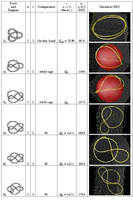
Figure 6: Table of results for the MC simulations of closed stiff knots. Three different configurations are found: (i) the circular braid for the $3_{1}$ knot; (ii) the 4-fold cage for the $4_{1}$ and $5_{2}$ knots (the sphere is a guide for the eye, indicating that this configuration is approximately wrapped around a sphere); (iii) the 80 for the $5_{2}$, $6_{2}$ and $6_{3}$.

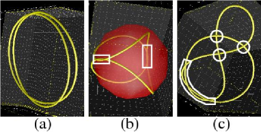
Figure 7: (a) The $3_{1}$ provides an example of line-braid of multiplicity 2. (b) The two contact zones in the 4-fold cage configuration are point-braids, indicated by white boxes. (c) An 80 configuration, exhibiting one point-braid and 3 double points, indicated by small circles.

A list of the knots studied in the simulations, together with the obtained equilibrium configurations, is presented in Fig.6. A knot is usually denoted with its crossing number $n_{c}$, and with an index which indicates its order in the standard list of knots for a given value of $n_{c}$. For the trefoil knot –denoted as $3_{1}$, which is a torus knot with $n=i=2$, the expected circular line-braid configuration is found, as shown on Fig.6. Fig.6 also shows two other configurations: the $4_{1}$ (figure 8 knot), and $5_{2}$ knots lead to a configuration which will be denoted as the 4-fold cage configuration in the following. The $5_{2}$, $6_{2}$, $6_{3}$ knots lead to a configuration which we call the 80 configuration (because it is composed of an 8 and a circle). The three different shapes are summarized on Fig.7. We observe that braid localization is present in all of them: line-braid for the $n=i$ configuration, and point braids for the two other configurations.

Figure 8: Knot families leading to 4-fold cage and 80. The boxes account for twists with an arbitrary number of turns.

In Fig.8, we have shown the conjectured knot families which lead to the 4-fold cage and the 80. These conjectured families are also reported on Fig.6. From knot tables knot-atlas , the sum of the 3 families $n=i$, 4-fold cage, and $80$ represent most of simple knots: all prime knots with $n_{c}<7$, and $75\%$ of those with $n_{c}<9$.

We have analyzed in details the energy of the 80 configuration. It is calculated from the procedure of sectionV.2. The structure of the 80 is composed of two parts: the 8, and the circle 0. The energy of the 8 curve is calculated in Appendix D: $\epsilon_{8}^{\circ}\approx 55.93$. The 0 is a circle, and its energy is $\epsilon_{0}^{\circ}=2\pi^{2}$. Since the 0 and the 8 are independent planar solutions, we may assume vanishing forces at their contact points, and analyze the structure of the 80 as a sum of two closed solutions (the 0 and the 8). Using Eq.(27), we may then evaluate the equilibrium energy of the 80 structure as:

$$\epsilon_{80}^{\circ}=(\epsilon_{8}^{\circ 1/2}+\epsilon_{0}^{\circ 1/2})^{2}\approx 142.1.$$ (38)

As expected from section V.1, the energy in the MC simulations (given on Fig.6), corresponding to a finite (but small) value of the width $w$, is slightly larger than the theoretical result corresponding to the limit $w\rightarrow 0$.

From the MC simulations, a normalized energy equal to $129.6$ is obtained for the 4-fold cage. Since $\partial_{w}{\cal E}^{*}_{w}>0$, this means that in the limit $w\rightarrow 0$, $\epsilon^{*}_{4C}<129.6$. The value of $\epsilon^{*}_{4C}$ is probably quite close to its numerical upper bound $129.6$, but we do not know its exact value. We only know from (31) that, since $n=2$, one has $\epsilon^{*}_{4C}>8\pi^{2}$. Finally, the different configurations relevant for the simulations fall into the hierarchy:

$$\epsilon^{\circ}_{CB}|_{i=2}<\epsilon^{\circ}_{4C}<\epsilon^{\circ}_{80}<\epsilon^{\circ}_{CB}|_{i=3}<\epsilon^{\circ}_{PBL}|_{n=2}\,.$$ (39)

As seen from Fig.6, some knots may exhibit more than one configuration. For example, both the 4-fold cage and the 80 configurations where observed with the $5_{2}$ knot. The hierarchy (39) shows that the 4-fold cage is the ground state, while the $80$ is metastable. This result is also observed in the simulations: although the energies of both configurations are slightly larger than the asymptotic value for $w\rightarrow 0$, their order is not affected by the finiteness of the width $w$.

VIII Open knots

Let us now consider an open knot, which exhibits two asymptotically straight open ends far from the knot as in Fig.1. We may ask the same question as for close knots: what are the configuration and the energy at equilibrium? We shall here show that our results on closed knots can be extended to the case of open knots.

Figure 9: Schematics of the open trefoil stiff knot. Open ends are along the $z$ axis. From left to right, the filament width $w$ decreases.

For an open knot, the total length of the string diverges. It is therefore more suitable to use the excess length ${\cal L}_{e}$, defined as the total length minus the length of a straight string:

$${\cal L}_{e}=\int ds(1-{\bf t}\cdot{\bf\hat{z}})=\int ds-\int dz$$ (40)

where the integrals are performed along the whole knot, and ${\bf\hat{z}}$ is the direction of the open ends far from the knot (We assume that both ends have the same direction). The excess length ${\cal L}_{e}$ should replace ${\cal L}$ in the expression of the energy ${\cal F}$ defined in Eq.(4). The variations are performed in the same way, and since the last term of (40) is constant, its variation vanishes, and the obtained differential system is the same as that for close knots.

Since open ends are straight, we assume that $\kappa\rightarrow 0$, and $\partial_{s}\kappa\rightarrow 0$ far from the knot. Then, from (20) we have ${\bf A.t}\rightarrow\mu^{\circ}$, ${\bf A.n}\rightarrow 0$, and ${\bf A.b}\rightarrow 0$. Since ${\bf A}$ describes internal forces in the string, and ${\bf t}$ is the tangent vector, this means that $\mu^{\circ}$ is the equilibrium tension far from the knot.

For a given structure $\{{\cal S}\}$ of an open knot at equilibrium, we show in Appendix C that the Lagrange multiplier $\mu^{\circ}$ is related to the curvature energy:

$$\mu^{\circ}_{\{{\cal S}\}}={{\cal E}^{\circ}_{\{{\cal S}\}}\over{\cal L}_{e}}=\epsilon^{\circ}_{e\{{\cal S}\}}{C\over{\cal L}_{e}^{2}}\,,$$ (41)

where the normalized energy of an open knot is defined as:

$$\epsilon^{\circ}_{e\{{\cal S}\}}={{\cal E}\over{\cal L}_{e}}\,.$$ (42)

The general expression of $\epsilon^{\circ}_{e\{{\cal S}\}}$ is given in Appendix C. Note that relation (41) is also valid for closed knots, as shown in section V.2.2. Since the excess length ${\cal L}_{e}$ is fixed, Eq.(41) also shows that the values of $\mu^{\circ}$ are ordered in the same way as the energies.

For open knots, the bridge number $n_{1}$ and the braid index $i_{1}$ are defined in the same way as for closed knots. If an open knot is obtained by opening a closed knot with bridge number $n$ and braid index $i$, the bridge number and braid index of the open knots are open-closed :

$$n_{1}=n-1\,,$$ (43)

$$i_{1}=i-1\,.$$ (44)

As an example, since $n=i=2$ for the trefoil knot, one has $n_{1}=i_{1}=1$ for the open trefoil knot.

The PBL configuration of Fig.3e with open ends connected to the knot via a straight line tangent to the point braid, is used as a first upper bound. A second upper bound is obtained with the circular braid configuration of Fig.3f with open ends connected to the knot via a straight line tangent to the circular line-braid. Finally, (32) and (41) are also valid for open knots when ${\cal L}$ is replaced by the excess length ${\cal L}_{e}$, so that the equilibrium tension $\mu^{*}$ of open knots obeys

$$2\pi^{2}n_{1}^{2}{C\over{\cal L}_{e}^{2}}\leq\mu^{*}\leq 2\pi^{2}\min[\alpha n_{1}^{2};i_{1}^{2}]{C\over{\cal L}_{e}^{2}}\,.$$ (45)

We therefore conclude that the equilibrium tension behaves as $n_{1}^{2}$, i.e. $\mu^{*}\sim n_{1}^{2}C/{\cal L}_{e}^{2}$. Furthermore, when $n_{1}=i_{1}$, the equilibrium shape of open knots is a circle tangent to a point braid, and $\mu^{*}=2\pi^{2}i_{1}^{2}C/{\cal L}_{e}^{2}$.

The simplest example of open knot is the open trefoil knot ($3_{1}$), for which $n_{1}=i_{1}=1$. As depicted in Fig.9, our theory predicts a circle tangent to a straight string in the limit $w\rightarrow 0$. This familiar shape is indeed easily obtained with a nylon string, a metal string, or hair. An example with a Silica nanowire is presented in Fig.1. The relation between tension and excess length $\mu^{*}=2\pi^{2}C/{\cal L}_{e}^{2}$ for the open trefoil knot was in fact already used as an ansatz in Ref.actin , where it was experimentally checked and used to evaluate the bending rigidity of actin. Here we show that it is an exact result in the limit $w\rightarrow 0$. Checking the $n^{2}$ dependence of $\mu^{*}$ by varying the knot type opens a novel and challenging line of investigations for experiments.

IX Discussion

In the following, we shall make some remarks, and briefly mention some open issues related to the present work.

IX.1 On the limits $w\rightarrow 0$ and ${\cal L}\rightarrow\infty$

Throughout the present paper, we have analyzed the limit $w\rightarrow 0$. Nevertheless, in a given experimental situation, it is difficult to perform a variation of the width of the filament. Furthermore, we have assumed that the bending rigidity modulus does not vary with the width. But it often does, as e.g. in continuum elasticityDoi , where $C\sim w^{-4}$. A more natural limit for experiments would be to take ${\cal L}\rightarrow\infty$ with fixed $w$. Both limits are equivalent. Indeed, the important point is that $w/{\cal L}\rightarrow 0$, as seen e.g. in the inequality (16).

IX.2 Curvature energy of thick knots

Two upper bounds for the energy of stiff knots can be derived from the limit of finite $w$. First, a general upper bound directly follows from excluded volume effects. Indeed, we have seen in section III that $\kappa\leq 2/w$. Hence,

$${\cal E}={C\over 2}\int ds\kappa^{2}\leq 2C{{\cal L}\over w^{2}}\,.$$ (46)

which may be re-written in terms of the dimensionless normalized energy:

$$\epsilon={{\cal E}C\over{\cal L}}\leq 2\left({{\cal L}\over w}\right)^{2}\,.$$ (47)

Using (15), one may also use ${\cal E}_{id}$ as an upper bound for the energy of a given knot. We do not know the precise value of ${\cal E}_{id}$, which is dictated by the geometry of the ideal knot. Nevertheless, a lower bound for ${\cal E}_{id}$ may be found from a recent conjecture based on results for lattice knotsErnst , which states that

$$\bar{\kappa}_{id}\geq b\,n_{c}^{1/2}$$ (48)

where $b$ is a positive constant. Using the Schwarz inequality as in section IV, we find that:

$${\cal E}_{id}\geq{b^{2}\over 2}n_{c}{C\over{\cal L}}$$ (49)

which may also be written as $\epsilon_{id}\geq b^{2}n_{c}/2$.

IX.3 Experimental shapes for stiff knots

We have performed rudimentary experiments in order to corroborate the results of our Monte Carlo simulations. We do not look for quantitative measurements, but we rather aim for a qualitative confirmation of the theory and simulations.

The experiments are performed with a plastic tube of width $w=1$cm, and length ${\cal L}=80$cm. To close the tube, we have joined the two ends using a small stick inserted in both ends. This closure allows tangential matching as well as free local rotation of one end with respect to the other at the contact point. Therefore, the tube cannot store twist, and the torsion energy is neglected. These experiments are imperfect, and cannot be used for quantitative purposes. For example, the small stick was less stiff than the tube, leading to a larger curvature at the junction. Moreover, the tube undergoes plastic deformation, and it did not come back to a straight shape after the experiments. Furthermore, solid friction occurs at the contact of the tube with itself. Therefore, the curvature energy of the tube may not be fully relaxed.

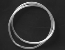
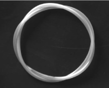
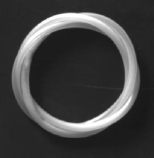
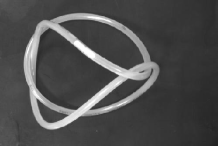
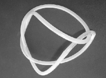
Figure 10: Photographs of closed knotted tube: $3_{1}$, $5_{1}$, $T(5,3)$ (torus knot), $4_{1}$, $5_{2}$ in 4-fold cage configuration, $5_{2}$ in 80 configuration.

Despite these imperfections, the experiments qualitatively confirmed the three types of shape already obtained, as shown on Fig.10. Circular braids are obtained for knots with $n=i$: $3_{1}$ and $5_{1}$, for which $i=2$, and also the $T(5,3)$ torus knot with $i=3$. Moreover, the expected 4-fold cage configuration is obtained for the $4_{1}$ and the $5_{2}$. Finally, 80 configurations is found for the $5_{2}$. These results are in perfect agreement with the results of the theory and the MC simulations of section VII.

IX.4 The restricted curvature problem

Other minimization problems share similarities with the minimization of the curvature energy ${\cal E}$. An example is the minimization of the total length of a knotted filament which exhibits a minimum possible radius of curvature $R_{+}$. This constraint may result from an excluded volume effect which limits the bending angle between adjacent units in a polymer or a macroscopic chain.

Let us assume that curvature $\kappa$ of a knotted filament cannot exceed $1/R_{+}$, i.e. $\kappa\leq 1/R_{+}$. Our aim here is to study the minimum possible length ${\cal L}^{\dagger}$ of this filament in the limit where $w\rightarrow 0$. First, from the inequality $\bar{\kappa}=\int ds\kappa\leq{\cal L}/R_{+}$ combined with (9), we obtain a lower bound for the length of a knot with a restricted curvature:

$${\cal L}\geq 2\pi nR_{+}.$$ (50)

Once again, we want to avoid angular points and knot localization, which exhibit infinite local curvature $>1/R_{+}$, and braid localization is expected in the limit $w\rightarrow 0$.

We then use the same strategy as before to determine upper bounds. A first upper bound is found from the PBL configuration, defined in Fig.3. Because of the discontinuous character of the constraint $\kappa\leq 1/R_{+}$, we cannot formulate the shape optimization problem with differential equations analogous to Eqs.(7,8) to obtain the minimal shape and energy. We therefore use a simple ansatz for the geometry, where loops are formed by arcs of circles. The precise shape is defined in Fig.11. The total length is:

$${\cal L}=2n\left[R_{1}(\pi+2\theta)+2R_{2}\theta\right]$$ (51)

where the free variables are $R_{1}$, $R_{2}$. The constraint of restricted curvature reads:

$$R_{1}\geq R_{+};\;\;R_{2}\geq R_{+}\,.$$ (52)

The angle $\theta$ is given by the relation:

$$R_{1}\cos(\theta)=R_{2}(1-\cos(\theta))\,,$$ (53)

with $0<\theta<\pi/2$. The minimization of ${\cal L}$ with the constraints is straightforward and leads to $R_{1}=R_{2}=R_{+}$, so that $\theta=\pi/3$. Therefore, the minimum length of the PBL configuration within our ansatz is:

$${\cal L}_{PBL}=2nR_{+}{7\pi\over 3}$$ (54)

Figure 11: Ansatz for the shape of the Point-Braid and Loop (PBL) configuration. The shape is made of arcs of circles of radius $R_{1}$, and $R_{2}$. The axis passing through the center of the circles goes through the contact point between two arcs, and defines the angle $\theta$.

A second upper bound for ${\cal L}^{\dagger}$ is deduced from the circular braid of radius $R_{+}$, whose length is $2\pi iR_{+}$. Finally, we obtain a result similar to (32):

$$2\pi nR_{+}\leq{\cal L}^{\dagger}\leq 2\pi\min\left[{7\over 3}n;i\right]R_{+}\,.$$ (55)

Similar conclusions are also drawn: Firstly, We conclude that the minimum length scales with the bridge number: ${\cal L}^{\dagger}\sim nR_{+}$. Secondly, the minimization problem is readily solved when $n=i$: we have ${\cal L}^{\dagger}=2\pi iR_{+}$ and the shape is a circular braid.

The restricted curvature problem was recently addressed numerically in Ref.Buck2004 for closed knots. As expected from the above result, the circular braid configuration was found for some torus knots (with $n=i=2$). A configuration similar to the 4-fold cage was also found for the $4_{1}$ knot. Whether both problems always lead to similar geometries is still an open question.

A second result of Ref.Buck2004 is that a transition occurs for a finite value of the width $w$ of the string. Does such a transition exist for stiff knots? Extensive simulations would be needed in order to answer this question.

X Conclusion

In summary, we find that stiff knot mechanics crucially depends on the type of knot via a surprisingly simple quantity: the bridge number $n$. Indeed both the equilibrium energy of closed knots and the equilibrium tension for open knots behave as $n^{2}$. Up to now, the open trefoil knot is the only knot which has been studied in experiments. More complex knots have been studied in the fluctuation dominated regime for polymers such as DNA Quake_Vilgis_Katrich . We hope that our results will motivate some numerical and experimental investigation of the mechanics of more complex stiff knots.

As a second central result, we find that braid localization, which was checked here on simple knots, is a general and robust feature of the entanglements of stiff strings. We shall mention two possible consequences of braid localization. Firstly, the curvature energy –and thus braid localization– should be irrelevant for flexible polymers. But it may be relevant for entanglements of semi-flexible polymers and fibers Morse2001 ; Rodney2005 ; actin-solutions . Imposing tangential contacts between the strings, braid localization questions the usual tube model for polymers, which is based on a lateral confinement due to simple crossingsMorse2001 . Secondly, braid localization also implies localization of friction and strain variations, and may have some important consequences on knot-induced polymer and filament break-up Saitta1999 ; actin .

Our work opens a new line of investigation towards the understanding of the geometry and mechanics of stiff knots. But much yet remains to be done, and we would therefore like to conclude with a list of open questions: (i) In the present work, we have essentially analyzed the equilibrium state. But we intuitively expect the number of metastable states to increase with the knot complexity. Can this be quantified? (ii) The question of the metastable states naturally leads to a second question: how can we study local stability (i.e. stability with respect to small perturbations)? (iii) We have studied the limit $w\rightarrow 0$. What happens for finite $w$? Here we have shown that the equilibrium energy ${\cal E}^{*}_{w}$ increases with $w$. The results of Buck and Rawdon Buck2004 on the similar restricted-curvature problem suggest that qualitative transitions may occur at finite $w$. (iv) As shown in basic textbooks such as Refs.Doi, , torsion usually plays an important role in filament mechanics. How can we include it in the present theory? We hope to report along these lines in the near future.

We wish to thank P. Peyla, Y. Colin de Verdière, S. Baseilhac, C. Lescop, M. Eisermann, and H. Meyer for helpful discussions. YCdV pointed out the proof of appendix B1.

Appendix A Monotonic increase of the equilibrium energy with $w$

In this section, we show that the curvature energy of a knotted string with tubular excluded volume strictly decreases as the diameter $w$ of the section of the tube decreases.

Figure 12: Excluded volume tubes of width $w_{1}$ and $w_{2}$.

To do so, let us consider a filament denoted as (1), of length ${\cal L}$, and with an excluded volume tube of width $w_{1}$. At equilibrium, the central line of the tube (1) is in the configuration ${\bf r}_{1}^{*}(s)$. Let us denote the energy of this configuration as ${\cal E}^{*}_{w_{1}}$. We then consider another filament of length ${\cal L}$, and of width $w_{2}$, with $w_{2}<w_{1}$. If the filament (2) is in the configuration ${\bf r}_{1}^{*}(s)$, the tube (2) is inside the tube (1). Therefore, there is no self-intersections or self-contact for the tube (2). Thus, there is no interactions of the tube (2) with itself. Hence, following the results of section III, ${\bf r}_{1}^{*}(s)$ is not the equilibrium configuration for the tube (2). Therefore, its energy ${\cal E}^{*}_{w_{1}}$ in the configuration ${\bf r}_{1}^{*}(s)$ is larger than the equilibrium energy ${\cal E}^{*}_{w_{2}}$ of the filament (2).

We have shown that ${\cal E}^{*}_{w_{2}}<{\cal E}^{*}_{w_{1}}$ when $w_{2}<w_{1}$, for any $w_{1}$ and $w_{2}$. As announced in the beginning of this section, ${\cal E}^{*}$ decreases as $w$ decreases –or equivalently $\partial_{w}{\cal E}^{*}>0$.

Appendix B Angle and knot localization

In this appendix, we show that the curvature energy of a curve in 3D diverges in the presence of angles, or knot localization. To do so, we will show the equivalent statement that, in the presence of an upper bound ${\cal E}_{0}$ for the energy:

$${\cal E}={C\over 2}\int ds\kappa^{2}<{\cal E}_{0}\,,$$ (56)

no angle or knot localization can be present.

Let us consider a part of the curve ${\bf r}(s)$, running from $s_{1}$ to $s_{2}$. From the Schwarz inequality and (56), one has:

$$\int^{s_{2}}_{s_{1}}ds\,\kappa \leq \left(\int^{s_{2}}_{s_{1}}ds\right)^{1/2}\left(\int^{s_{2}}_{s_{1}}ds\,\kappa^{2}\right)^{1/2}$$ (57)

$$\leq (s_{2}-s_{1})^{1/2}\left({2{\cal E}_{0}\over C}\right)^{1/2}$$

B.1 Angles

We observe that:

$$|{\bf t}(s_{2})-{\bf t}(s_{1})| = \left|\int^{s_{2}}_{s_{1}}ds\,\partial_{s}{\bf t}\right|$$ (58)

$$= \left|\int^{s_{2}}_{s_{1}}ds\,\kappa{\bf n}\right|\leq\int^{s_{2}}_{s_{1}}ds\,\kappa$$

where $({\bf t},{\bf n},{\bf b})$ is the usual Frenet frame along the curve. Combing (57) and (58), we obtain:

$$|{\bf t}(s_{2})-{\bf t}(s_{1})|\leq(s_{2}-s_{1})^{1/2}\left({2{\cal E}_{0}\over C}\right)^{1/2}$$ (59)

Eq.(59) shows that the tangent vector ${\bf t}$ is continuous along the curve. Therefore, no angle can be present.

B.2 Knot localization

If the part of the knot between $s_{1}$ and $s_{2}$ is knotted, then there is a lower bound for the total curvature which is similar to Eq.(9). But since the knot is an open one, one should use the modified bridge number defined in section VIII, which we denote as $n_{1\rightarrow 2}$. We thus have:

$$\int^{s_{2}}_{s_{1}}ds\,\kappa\geq 2\pi n_{1\rightarrow 2}$$ (60)

Using this inequality together with (57), we obtain:

$$n_{1\rightarrow 2}\leq{1\over 2\pi}\left({2{\cal E}_{0}\over C}\right)^{1/2}(s_{2}-s_{1})^{1/2}$$ (61)

Knot localization means that there is a knot between $s_{1}$ and $s_{2}$ while $(s_{1}-s_{2})\rightarrow 0$. But (61) shows that, as $(s_{2}-s_{1})\rightarrow 0$, one necessarily has $n_{1\rightarrow 2}=0$. Since $n_{1\rightarrow 2}=0$ corresponds to an unknotted string, there is no knot localization.

Appendix C Some relations for a structure of line-braids

C.1 Closed knots

C.1.1 Relation between ${\cal E}$ and $\mu$

We here derive a relation between ${\cal E}$, ${\cal L}$, and $\mu$. Integrating (21) over the $p$th line-braid, we obtain:

$${\cal E}^{\circ}_{p}-\mu^{\circ}m_{p}{\cal L}^{\circ}_{p}={\bf A}_{p}.[{\bf r}]_{p}$$ (62)

where $[{\bf r}]_{p}$ is the difference between ${\bf r}$ at the beginning and at the end of the line-braid. Summing (62) over $p$, we obtain:

$${\cal E}^{\circ}-\mu^{\circ}{\cal L}=\sum_{p=1}^{N}{\bf A}_{p}.[{\bf r}]_{p}=\sum_{B}{\bf r}_{B}.\sum_{p\rightarrow B}{\bf A}_{p}=0$$ (63)

where the last equality follows from (24). Finally, one has:

$$\mu={{\cal E}\over{\cal L}}$$ (64)

This equality is true for all structures which obey (21,22), with the boundary conditions (24,25).

C.1.2 Expression of $\epsilon$

We now derive a relation between the total normalized energy, and the normalized energy of its parts. Eliminating $\mu$ between Eqs.(62) and (64), and rewriting energies in terms of the normalized energies $\epsilon$, we find

$$m_{p}\left(\epsilon_{p}^{\circ}-{\bf A}_{p}.[{\bf r}]_{p}{{\cal L}_{p}\over m_{p}C}\right)^{1/2}=\epsilon^{\circ 1/2}_{\{{\cal S}\}}{m_{p}{\cal L}_{p}\over{\cal L}}$$ (65)

where $\epsilon_{p}={\cal E}_{p}{\cal L}_{p}/m_{p}C$. Summing over $p$, we get:

$$\epsilon^{\circ 1/2}_{\{{\cal S}\}}=\sum_{p=1}^{N}m_{p}\left(\epsilon^{\circ}_{p}-{\bf A}_{p}.[{\bf r}]_{p}{{\cal L}_{p}\over m_{p}C}\right)^{1/2}\,.$$ (66)

There are three interesting cases in which the second term in the parenthesis vanishes. The first one is the situation where line-braids are arcs of circles, for which ${\bf A}_{p}=0$. In the second case, all line-braids are loops (i.e. they start and end at the same point), implying $[{\bf r}]_{p}=0$. The third case is the case where all line-braids have identical energies and length. If there is $N$ line-braids, $\mu={\cal E}/{\cal L}=N{\cal E}_{p}/Nm_{p}{\cal L}_{p}={\cal E}_{p}/m_{p}{\cal L}_{p}$. Such an equality, combined with (62), implies that ${\bf A}_{p}.[{\bf r}]_{p}=0$. In these 3 cases, one finally has:

$$\epsilon_{\{{\cal S}\}}^{\circ}=\Bigl{[}\sum_{p}m_{p}\epsilon_{p}^{\circ 1/2}\Bigr{]}^{2}\,,$$ (67)

and from Eq.(65), one finds Eq.(28).

C.2 Open knots

C.2.1 Relation between ${\cal E}$ and ${\cal L}_{e}$

In the case of open knots, the relation (62) is still valid for each line-braid. But the sum in (63) does not vanish, and we obtain:

$${\cal E}^{\circ}-\mu^{\circ}{\cal L}^{\circ}=\sum_{p=1}^{N}{\bf A}_{p}.[{\bf r}]_{p}=\sum_{B}{\bf r}_{B}.\sum_{p\rightarrow B}{\bf A}_{p}=[{\bf r}.{\bf A}]_{-}^{+}$$ (68)

where the index $\pm$ indicate the two open ends at $z_{\pm}\rightarrow\pm\infty$. Using Eq.(20), we obtain

$$[{\bf r}.{\bf A}]_{-}^{+}\rightarrow-\mu^{\circ}z_{+}+\mu^{\circ}z_{-}=-\mu\int dz,$$ (69)

so that (68) can be re-written as:

$$\mu={{\cal E}\over{\cal L}_{e}}\,,$$ (70)

where ${\cal L}_{e}$ is defined in Eq.(40).

C.2.2 Expression of $\epsilon_{e}$

Let us denote with the index $+$ and $-$ the parts of the structure related to the open ends. Their excess lengths ($\int ds-\int dz$ along these parts) are respectively denoted as ${\cal L}_{e+}$ and ${\cal L}_{e-}$. The $+$ part extends from $z_{+}\rightarrow+\infty$ to the first contact point, whose abscissa along $z$ is denoted as $z_{0+}$. For the $-$ part, $z_{0-}$ is defined in a similar way. We then define $\Delta_{0}=z_{0+}-z_{0-}$.

Following the same lines as in the previous paragraphs, one finds that:

$$\epsilon_{e+}^{\circ}=\epsilon_{e}^{\circ}\left({\cal L}_{e+}^{\circ}\over{\cal L}_{e}\right)^{2}\;\;\;\epsilon_{e-}^{\circ}=\epsilon_{e}^{\circ}\left({\cal L}_{e-}^{\circ}\over{\cal L}_{e}\right)^{2}$$ (71)

$$\epsilon_{p}^{\circ}=\epsilon_{e}^{\circ}\left({\cal L}_{p}^{\circ}\over{\cal L}_{e}\right)^{2}+{\bf A}_{p}.[{\bf r}]_{p}{{\cal L}_{p}^{\circ}\over m_{p}C}$$ (72)

Summing these relations over all line-braids lead to:

$$\left(1+{\Delta_{0}\over{\cal L}_{e}}\right)\epsilon^{\circ 1/2}_{e}$$ (73)

$$= \sum_{p=1}^{N}m_{p}\left(\epsilon_{p}^{\circ}-{\bf A}_{p}.[{\bf r}]_{p}{{\cal L}_{p}\over m_{p}C}\right)^{1/2}+\epsilon_{e+}^{\circ 1/2}+\epsilon_{e-}^{\circ 1/2}\,.$$

Appendix D Energies of special configurations

D.1 Energy of the planar loop

In this appendix, we determine the energy of one planar loop in the configuration of Fig.3e. For planar solutions, ${\bf A}$ is parallel to the plane, and Eqs.(7,8) reduce to:

$${1\over 2}(\partial_{s}\theta)^{2}-{1\over C}(\mu+A\cos\theta)=0\,,$$ (74)

where $A=|{\bf A}|$, and $\theta$ is the angle between the tangent vector ${\bf t}$ and ${\bf A}$.

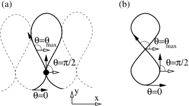
Figure 13: Schematics of (a) the loop solution. The loop part of solution used in the text starts and ends at the place indicated by the black dot. (b) the 8 solution.

The abscissa $x$, defined in Fig.13, is written as:

$$x=\int^{x}_{0}dx=\int_{0}^{\theta}d\theta{\partial_{s}x\over\partial_{s}\theta}=\int_{0}^{\theta}d\theta{\cos\theta\over\partial_{s}\theta}\,,$$ (75)

where $\partial_{s}\theta$ is given by Eq.(74). Using the variable change $v=-\alpha\cos\theta$, with $\alpha=A/\mu$, we find:

$$x=\alpha^{-1}\left(C\over\mu\right)^{1/2}\int_{v}^{\alpha}{v\,dv\over(\alpha^{2}-v^{2})^{1/2}(v+1)^{1/2}}\,.$$ (76)

As seen from an inspection of Fig.13a, the constraint which selects the loop solution with a tangent vector along $y$ at the boundary is:

$$x(\theta=\pi/2)-x(\theta=0)=2(x(\theta=\pi/2)-x(\theta_{max})),$$ (77)

where $\theta_{max}$ is such that $v_{max}=-1$. This constraint leads to an equation for $\alpha$:

$$2\int_{-1}^{0}{v\,dv\over(\alpha^{2}-v^{2})^{1/2}(v+1)^{1/2}}$$

$$+\int_{0}^{\alpha}{v\,dv\over(\alpha^{2}-v^{2})^{1/2}(v+1)^{1/2}}=0\,.$$ (78)

Moreover, since $\kappa=|\partial_{s}\theta|$, the energy reads:

$${\cal E}_{loop}={C\over 2}\int ds(\partial_{s}\theta)^{2}\,,$$ (79)

and the total length is:

$${\cal L}_{loop}=\int ds\,.$$ (80)

These integrals are both re-written with the new variable $v$, and finally the normalized energy reads:

$$\epsilon_{loop}^{\circ} = {{\cal E}_{loop}{\cal L}_{loop}\over C}$$ (81)

$$= 2\left[2\int_{-1}^{0}dv{(v+1)^{1/2}\over(\alpha^{2}-v^{2})^{1/2}}+\int_{0}^{\alpha}dw{(v+1)^{1/2}\over(\alpha^{2}-v^{2})^{1/2}}\right]$$

$$\times\left[2\int_{-1}^{0}{dv\over(\alpha^{2}-v^{2})^{1/2}(v+1)^{1/2}}\right.$$

$$\hskip 8.5359pt\left.+\int_{0}^{\alpha}{dv\over(\alpha^{2}-v^{2})^{1/2}(v+1)^{1/2}}\right]\,.$$

The numerical solution of Eq.(78) leads to $\alpha\approx 2.158$. Substituting this value in Eq.(81), we find $\epsilon_{loop}^{\circ}\approx 18.19$.

D.2 Energy of the 8

For the ’8’, we use the same method as in the previous section. The constraint is now the periodicity of the curve, which imposes

$$x(\theta_{max})=x(-\theta_{max})\,,$$ (82)

where $\theta_{max}$ is the maximum angle reached along the curve. This leads to the following condition after the change of variable to $v$:

$$\int_{-1}^{\alpha}{v\,dv\over(\alpha^{2}-v^{2})^{1/2}(v+1)^{1/2}}=0\,,$$ (83)

which is solved numerically, and leads to $\alpha=1.53$. Moreover,

$$\epsilon_{8}^{\circ} = {{\cal E}_{8}{\cal L}_{8}\over C}$$ (84)

$$= 8\left[\int_{-1}^{\alpha}dv{(v+1)^{1/2}\over(\alpha^{2}-v^{2})^{1/2}}\right]$$

$$\times\left[\int_{-1}^{\alpha}{dv\over(\alpha^{2}-v^{2})^{1/2}(v+1)^{1/2}}\right]\,.$$

We find numerically that $\epsilon_{8}\approx 55.93$.

References

- (1) Y. Arai et al Nature 399 446 (1999).
- (2) T. Lobovkina et al, PNAS 101 7949 (2004).
- (3) B. Vigolo et al Science, 290 1331 (2000).
- (4) L. Tong et al, Nature 426, 816 (2003).
- (5) A.M. Saitta et al, Nature 399 46 (1999).
- (6) X. R. Bao et al Phys. Rev. Lett. 91, 265506 (2003); M. Otto and T. A. Vilgis Phys. Rev. Lett. 80, 881-884 (1998); V. Katrich et al Nature 384 142 (1996).
- (7) D. C. Morse, Phys. Rev. E 63, 031502 (2001).
- (8) D. Rodney, M. Fivel, and R. Dendievel Phys. Rev. Lett. 95, 108004 (2005).
- (9) B. Hinner et al, Phys. Rev. Lett. 81 2614 (1998); M.L. Gardel et al Phys. Rev. Lett. 91 158302 (2003).
- (10) E Guitter and E Orlandini, J. Phys. A, 32 1359 (1999); R. Metzler, A. Hanke, P.G. Dommersnes, Y. Kantor, and M. Kardar,Phys. Rev. Lett.88, 188101 (2002).
- (11) P. G. Dommersnes et al, Phys. Rev. E 66, 031802 (2002).
- (12) J. O’Hara, Energy of knots and conformal geometry, World Scientific, Singapore (2003).
- (13) see e.g. L.D. Landau and E.M. Lifshitz, Course of Theoretical Physics, vol.7, 17 Butterworth and Heinemann (1999), or M. Doi and S.F. Edwards, The theory of polymer dynamics; Cambridge Univ. Press (1986).
- (14) L. Euler, Bousquet, Lausannae et Genevae 24, E65A. O.O.Ser.I (1744).
- (15) J. Langer and D.A. Singer, J. London Math. Soc. (2) 30 512 (1984).
- (16) H. von der Mosel, Asymptotic Anal. 18, 49 (1998).
- (17) J.W. Milnor, Ann. of Math. (2) 52, 248 (1949).
- (18) R.D. Kamien, Rev. Mod. Phys., 74 953 (2002).
- (19) P.G. De Gennes, Macromolecules, 17, 703 (1984); P. Pierański, S. Przybyl, and A. Stasiak, Eur. Phys. J. 6, 123 (2001).
- (20) V. Katrich et al Nature 384 142 (1996); V. Katrich et al Nature 388 148 (1997).
- (21) J.W. Alexander, Proc. Nat. Acad. Sci., USA 9 93 (1923).
- (22) L.H. Kauffman, Knots and Physics, World Scientific Singapore (1993).
- (23) http://katlas.math.toronto.edu/
- (24) SA. Wasserman and NR. Cozzarelli, Science 232 951 (1986).
- (25) C. Lescop, private communication.
- (26) Y. Diao and C. Ernst, to appear in Proceedings of Cambridge Phil. Soc. (2006).
- (27) G. Buck and E.J. Rawdon Phys. Rev.E 70 011803 (2004).