Density matrix renormalization on random graphs and the quantum spin-glass transition

Abstract

The density matrix renormalization group (DMRG) has been extended to study quantum phase transitions on random graphs of fixed connectivity. As a relevant example, we have analysed the random Ising model in a transverse field. If the couplings are random, the number of retained states remains reasonably low even for large sizes. The resulting quantum spin-glass transition has been traced down for a few disorder realizations, through the careful measurement of selected observables: spatial correlations, entanglement entropy, energy gap and spin-glass susceptibility, among others.

I Introduction

Quantum phase transitions constitute a very active topic in theoretical physics Sachdev (2001), to which disorder and frustration of a quantum spin glass add considerable intricacies Rieger (2005). Although quantum effects were usually considered to be negligible in spin glasses at finite temperatures, diverse experiments Wu et al. (1993); MacLaughlin et al. (2001); Chen et al. (2005) have proved them to be highly relevant, leading to the first experimental realization of quantum annealing Brooke et al. (1999). One of the most widely employed theoretical approaches to the quantum spin-glass transition (QSGT) is the random couplings Ising model in a transverse field (RITF) Chakrabarti et al. (1996). Within the analytical approach, a Griffiths phase was found in the 1D case via an elegant RG procedure Fisher (1995); Fisher and Young (1998), while such a structure was proved to be absent from the infinite range case within the replica formalism Bray and Moore (1980); Goldschmidt and Lai (1990); Miller and Huse (1993). The 1D RG analysis was extended to study the presence of a certain number of long-distance links, proving the relevance of the perturbation Carpentier et al. (2005). Regarding numerical approaches, quantum Monte-Carlo (QMC) remains as the most suitable tool at $T>0$. Using it, a coherent picture was obtained in the 2D and 3D cases, showing that the Griffiths phase is present in 2D but absent in 3D Guo et al. (1994); Rieger and Young (1994, 1996).

Classical spin glasses have been thoroughly analysed on Bethe lattices Thouless (1986). However, finite Bethe lattices are dominated by boundary effects and present no frustration. A way out is to study random graphs with a fixed connectivity which, in the classical case, allow the application of the cavity approach Mézard and Parisi (2001). These random graphs present genuine frustration, since they have loops, and have no boundaries. On the other hand, the average size of the loops grows with the number of sites Marinari and Monasson (2004), thus making them resemble, locally, a Bethe lattice (see figure 1).

The density matrix renormalization group (DMRG) White (1992); Schollwöck (2005) is known to be a highly accurate method to analyze $T=0$ ground state properties of 1D or quasi-1D quantum many body systems, including tree structures Martín-Delgado et al. (2002). We have extended the method in order to trace the behaviour of finite size samples of random graphs of fixed connectivity $K=3$ across the QSGT within the RITF model. Given the high connectivity of these graphs, the applicability of the DMRG is highly non-trivial. It is remarkable that in the case of non-random couplings, we have found the number of retained states needed to ensure a good accuracy to be very high, rendering the application of the DMRG unfeasible.

The careful analysis of pseudo-critical points of finite size samples constitutes a powerful tool to study a QSGT. As a recent example, the work of Iglói and coworkers Iglói et al. (2007) studies the distributions of, e.g., the average entanglement entropy and the surface magnetization of finite size 1D samples. In this work we provide measurements of, among other observables, spin-glass susceptibilities, energy gaps, long distance spin-spin correlations and entanglement entropies, and use them to obtain insight on the mechanism of the transition. A full characterization of the QSGT, nonetheless, is not attempted in this work, since it would require to obtain statistics on a large number of disorder realizations.

The rest of the paper is organized as follows: Sec. II presents the model, and Sec. III provides details on the application of DMRG. Sec. IV shows the numerical DMRG results obtained. Sec. V presents a discussion of the results and some concluding remarks.

II Model

Let us consider the random Ising model in a transverse Field (RITF) on a generic graph Chakrabarti et al. (1996):

$$H=-\sum_{\left<i,j\right>}J_{ij}\sigma^{z}_{i}\sigma^{z}_{j}-\sum_{i}h^{z}_{i}\sigma^{z}_{i}-\Gamma\sum_{i}\sigma^{x}_{i}\;,$$ (1)

where $\left<i,j\right>$ denotes pairs of neighboring sites $i$ and $j$ on the graph. The values of $J_{ij}$ are uncorrelated random variables with a uniform probability density distribution in the interval $[-1,1]$. We will focus our study on randomly generated graphs, with $N$ sites and a fixed connectivity $K=3$ Mézard and Parisi (2001); Marinari and Monasson (2004), i.e., each site $i$ is connected to $K=3$ other (randomly chosen) sites $j$. An example of such a graph, with $N=30$ sites, is shown in Fig. 1.

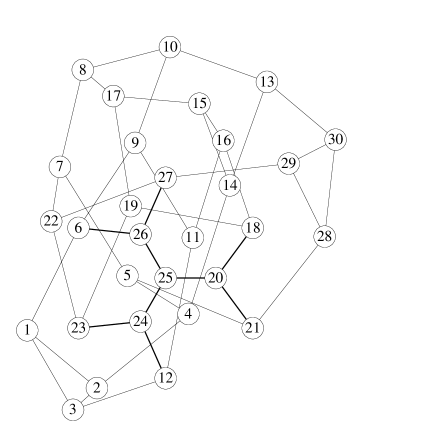
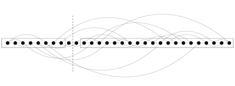
Figure 1: (a) A random graph with $N=30$ sites and connectivity $K=3$. Stronger bonds highlight the local Bethe lattice structure around site 25. Numerical labels denote the order in which they are visited along the DMRG path. (b) Deformation of the same graph to show the DMRG path as a straight line. The left and right blocks at a certain DMRG step are shown, and the dashed line cuts all the long-range links that would need reconstruction during that DMRG step, 9 in the example.

It should be noticed that, locally and for large $N$, such graphs resemble Bethe lattices, as we have highlighted with thicker links in Fig. 1. Nonetheless, the behaviour of finite Bethe lattices is dominated by the boundary, unlike in our case, where there is none. Moreover, trees have no loops and, therefore, present no frustration, while random graphs with fixed connectivity do contain loops and, therefore, have genuine frustration. It has been proved, nonetheless, that short loops become rare as $N\to\infty$: More precisely, the probability of finding a loop of any fixed size $L$ falls to zero when $N\to\infty$ Marinari and Monasson (2004). The physics of classical spin glasses in these graphs has been studied using the cavity method by Mézard and Parisi Mézard and Parisi (2001).

Let $\epsilon_{N}$ be the absolute value of the disorder-averaged energy per site of the classical ground state. Our numerical experiments show that it increases from $\sim 0.6$ at $N=100$ up to $\sim 3/4$ for larger $N$, which is the theoretical limiting value for $N\to\infty$ under the assumption that all links are satisfied.

We will take the product of eigenstates of $\sigma^{z}_{i}$, for all $i$, as the canonical basis for our problem. In this basis, we denote the state in which all spins point in the positive $x$-direction as $\left|\hat{x}\right>\equiv 2^{-N/2}\prod_{i}(\left|\uparrow\right>+\left|\downarrow\right>)$. Let us assume, for the moment, that $h^{z}_{i}=0$ for all $i$. For $\Gamma=0$, all the non-diagonal terms in the Hamiltonian vanish. Therefore, the ground state is given by the configurations with the classical minimum energy. Disregarding accidental degeneracies, there are two such configurations, related by a simultaneous flip of all spins, $\sigma_{i}^{z}\to-\sigma_{i}^{z}$ for all $i$. The transverse field $\Gamma$ may be considered as a kinetic energy coefficient, providing a hopping term among the classical configurations. In the $\Gamma\to\infty$ limit the transverse field term dominates and the ground state tends to the state $\left|\hat{x}\right>$, with all the spins pointing in the positive $x$-direction, separated by a large gap $\Delta\approx 2\Gamma$ from the first excited state. Let us remark that all the components of the canonical basis have the same amplitude in the state $\left|\hat{x}\right>$.

By decreasing $\Gamma$ there is a certain value $\Gamma=\Gamma_{c}$ for which the system undergoes a quantum spin-glass transition (QSGT). For $\Gamma>\Gamma_{c}$, the system is in a quantum paramagnetic phase, which presents no long-range order. Below $\Gamma_{c}$, the system is in a quantum spin-glass phase, presenting a hidden long-range order which may be detected by a number of observables. We will focus here on the divergence of the spin-glass susceptibility:

$$\chi_{SG}\equiv\frac{1}{N}\sum_{ij}\left(\frac{\partial\left<\sigma^{z}_{i}\right>}{\partial h^{z}_{j}}\right)^{2}\;,$$ (2)

i.e., physically, a small longitudinal magnetic field $h^{z}_{j}$, applied at site $j$, generates a magnetization response on each site $i$, which is measured (and squared, so as to disregard its sign); the results are summed over all sites $i$ and averaged over all sites $j$. If the system is in a paramagnetic phase, the magnetization will be proportional to $h^{z}_{j}$ and short-ranged in space, so that the sum over $i$ and $j$ yields a finite value for $\chi_{SG}$. On the other hand, on approaching the spin-glass phase, an infinitesimally small longitudinal magnetic field $h^{z}_{j}$, localized at a single site $j$, will eventually induce a finite magnetization over a long-range of spins. This effect is at the origin of the divergence of $\chi_{SG}$.

We shall now discuss the numerical approach we have used to study this system, and the results obtained.

III Application of the DMRG

The density-matrix renormalization group (DMRG) has proved to be an accurate method to analyse the properties of 1D and quasi-1D systems White (1992); Schollwöck (2005); Martín-Delgado et al. (2002). The DMRG may be described as a variational method within the matrix-product states (MPS), which constitute a low-dimensional subspace of the full Hilbert space Rommer and Östlund (1997). A MPS may be expressed as

$$\left|\Psi\right>=\sum_{s_{1}\cdots s_{N}}{\rm Tr}\left(A^{(s_{1})}\cdots A^{(s_{N})}\right)\left|s_{1}\cdots s_{N}\right>\;,$$ (3)

where each $A^{(s_{i})}$ is a square matrix with dimension $m$, which may be considered as the number of retained states per block when splitting the system into a left and right parts. The total number of variational parameters is less than $2Nm^{2}\ll 2^{N}$. The success of the DMRG is related to the ability of these MPS to reproduce faithfully the ground states of local 1D many-body problems for low values of $m$ Verstraete and Cirac (2006). If $m\to\infty$, any state of the Hilbert space may be exactly represented as a MPS.

The minimum number of retained states $m$ is related to the exponential of the von Neumann entanglement entropy of the DMRG block Vidal et al. (2002). In a non-critical 1D system, this entropy is bounded for all sizes, while it grows as $\ln L$ for a 1D critical system of length $L$. It is believed that for a $D$-dimensional system out of criticality, the entanglement entropy scales as $L^{D-1}$, where $L$ is the shortest spatial dimension of the system Sredniki (1993). This estimate is known as the area law and is believed to have logarithmic corrections at critical points. An important practical consequence is that, in order to study a 2D system, the number of retained states $m$ should grow as $\exp(L)$, thus making the DMRG very inefficient.

Our system, on the other hand, is defined on a random graph of fixed connectivity, $K=3$. We will show that this poses no problem to the number of retained states $m$, which appears to remain manageable even for $N=500$ as long as the couplings are random. However, the implementation of the DMRG on such a model has required the following technical refinements of the original method:

(a) Path selection.

In a non-1D system, DMRG proceeds by converting the system into an effective 1D problem with long-range couplings. A path is chosen along the graph, which does not repeat sites, and is considered to be appropriate if the number of broken links between the left and the right blocks is kept low along a DMRG sweep. Normally, the selection of a suitable path in a quasi-1D system (e.g. ladders) is done by geometrical intuition. In our implementation we have designed an automated procedure: a simulated annealing algorithm is employed in order to minimize the number of broken links. The full problem of finding the optimal path is computationally very hard. Therefore, we do not aim at the exact optimum, but only to a reasonably good local minimum. We have noticed that our quasi-optimal path performs much better than a random path.

(b) Perron-Frobenius criterion.

The Hamiltonian of the RITF on any graph fulfills, on the canonical basis, the conditions of the Perron-Frobenius theorem, i.e., all off-diagonal components are non-positive. Hence, all the ground state components must have the same sign. Using the MPS representation of the ground state obtained within the DMRG, it is always possible to reconstruct the amplitude of any configuration $C=\{s_{1}\cdots s_{N}\}$. The obtention of the full $\left|\Psi\right>$ is unfeasible, since it would require reconstructing the amplitude of an exponentially large number of configurations. Nonetheless, it is possible to pick up a few random configurations $C$, and check that all their amplitudes have the same sign. Whenever this criterion was not met —a rather rare event—, the calculation was repeated changing the random seed for the Lanczos procedure on the first DMRG step.

(c) Wavefunction annealing.

For large $\Gamma$ the ground state $\left|\hat{x}\right>$ is easily representable as a MPS, requiring a single retained state. The DMRG works extremely well in this regime and, therefore, our simulations are always started well within the paramagnetic (large $\Gamma$) phase. The QSGT is approached by repeatedly decreasing the value of $\Gamma$ by a small amount, always using the previous ground state as a seed for the new calculation, exploiting the wavefunction transformations suggested by White White (1996). This type of annealing of the ground state provides a faster convergence and more accurate results for low $\Gamma$.

(d) Adaptive number of retained states.

The number of retained states $m$, and the number of DMRG sweeps $n_{s}$, are not fixed in our algorithm. We set a maximum value for the sum of the neglected eigenvalues of the density matrix in the RG truncation ($\eta\approx 10^{-6}$), and select $m$ accordingly. Moreover, sometimes convergence takes more sweeps than usual ($n_{s}\approx 30-40$) in order to obtain machine precision in the convergence of the ground state energy.

(e) Energy gap measurements.

When there is a symmetry in a problem, e.g., under SU(2), it is usually possible to obtain the first excited state as the ground state of a different sector of the Hilbert space. In our case, lacking this, the best option has proved to be the following one. For each DMRG step, after the ground state $\left|\Psi_{0}\right>$ had been found, it was “promoted” to a higher energy by the following transformation of the Hamiltonian:

$$H\to H+\lambda\left|\Psi_{0}\right>\left<\Psi_{0}\right|\;,$$ (4)

in such a way that the ground state of this new hamiltonian is the former first excited state, as long as we take $\lambda>\Delta$, $\Delta$ being the gap we are looking for. The density matrix used for truncation was built as a linear combination of the density matrices for each state, with equal weights. However, we should remember that only ground states of local Hamiltonians are expected to be faithfully represented by MPS Verstraete and Cirac (2006), and Eq. (4) does not define a local Hamiltonian. Therefore, the accuracy in the gap estimate is worse than that in the ground state energy and in other observables.

IV Results

We have applied the modified DMRG technique to study a few samples of random graphs with fixed connectivity $K=3$ and sizes ranging from $N=50$ to $N=500$.

A full characterization of the QSGT would require relevant statistics on the disorder. Unfortunately, in order to obtain a high accuracy for each sample, the required CPU-time is rather large. Therefore, we have decided to focus on a precise study of a few realizations, in order to gain insight on the mechanism of the transition for finite samples. Most of our findings will be illustrated in the figures of this section by showing in detail the results obtained for a sample with $N=200$ sites. It should be remarked that the highlighted features are typical of all the ensemble.

The numerical simulations were done with the DMRG algorithm explained in section III, with a neglected probability tolerance $\eta=10^{-6}$ and a tolerance on the convergence of the energy of one part in $10^{10}$, for ten samples of each size ($N=$ 50, 100, 150, 200, 250, 300, 400, 500). Each sample is a different random graph, always with fixed connectivity $K=3$, and the bonds $J_{ij}$ are random and independent, uniformly distributed in the interval $[-1,1]$.

Figure 2(a) shows three observables calculated for a given instance of a $N=200$ graph, as a fuction of $\Gamma$. The most relevant quantity is the spin-glass susceptibility, defined in equation 2. A small magnetic field $h^{z}_{i_{0}}=10^{-4}$ is applied at a single site $i_{0}$, and the magnetic response is measured with the formula

$$\chi^{(i_{0})}_{SG}\equiv\sum_{j}\left(\frac{\left<\sigma^{z}_{j}\right>}{h^{z}_{i_{0}}}\right)^{2}\;,$$ (5)

which is found to increase very fast as $\Gamma$ approaches $1.28$ from above, and thereupon saturating at a very high value. Figure 2(b) proves the divergence of $\chi_{SG}$ by showing its behavior at three different values of $h^{z}_{i_{0}}$ ($h^{z}_{i_{0}}=10^{-3}$, $10^{-4}$ and $10^{-5}$): the saturation value is seen to scale as $1/(h^{z}_{i_{0}})^{2}$. We estimate the pseudo-critical value $\Gamma_{c}$ for the given sample as the value of $\Gamma$ at which the slope of the susceptibility attains its maximum. With this definition, $\Gamma_{c}$ appears to be almost independent of the chosen site $i_{0}$, at our level of precision $\Delta\Gamma=\pm 0.01$. Figure 2(c), finally, shows $\chi_{SG}$ for ten different samples with $N=200$ sites, differing in the graph structure and in the choice of the couplings $J_{ij}$, and diverging at different (sample dependent) values of $\Gamma_{c}$.

Figure 2(a) also shows two other observables which point towards the same value for $\Gamma_{c}$. The first is the block entanglement entropy, defined as $S\equiv-{\rm Tr}(\rho\log(\rho))$, where $\rho$ is the reduced density matrix for a part of the system. It is measured for all the left-right decompositions along a DMRG sweep, and its maximum value is denoted by $S_{max}$. This value of $S_{max}$ is obviously dependent on the DMRG path. Nonetheless, since this path has been chosen so as to minimize the number of retained states, it is expected that it will also minimize the maximum value of the entropy. It should be emphasized that this observable attains its maximum value, as a function of $\Gamma$, at the same $\Gamma_{c}$ which is found by analyzing the spin-glass susceptibility. The relevance of the entanglement entropy in order to characterize the critical point of a QSGT has already been remarked in the literature Iglói et al. (2007). The DMRG, being based on the obtention and analysis of the density matrix of different parts of the system, is specially well suited for measuring this observable de Chiara et al. (2006).

The other observable shown in figure 2(a) is the energy gap $\Delta$, which extrapolates to zero at a value of $\Gamma$ which is close to $\Gamma_{c}$. The sign of the difference between these two pseudo-critical points is sample dependent. This discrepancy is likely to be a finite size effect.

Figure 2: (a) For a random sample with $N=200$ sites, the spin-glass susceptibility $\chi_{SG}$ is shown in logarithmic scale, along with the maximum block entropy $S_{max}$ and the energy gap $\Delta$, the two latest in arbitrary units. The divergence of $\chi_{SG}$ is marked with the vertical line, which clearly coincides with the maximum value of $S_{max}$. The energy gap comes very close to zero (dotted line) precisely in that region. (b) The fact that $\chi_{SG}$ saturates is related to the finite value of the applied $h^{z}$ field. In this figure we can see how this saturation value increases as $h^{z}$ is decreased. (c) The divergence of $\chi_{SG}$ is shown for several samples, all with $N=200$ sites.

The next observable that we calculated for each sample is the average value of $\left<S^{x}\right>$, see figure 3. For high $\Gamma$, the transverse field is dominant, the ground state is close to $\left|\hat{x}\right>$ and the value of $\left<S^{x}\right>$ is close to 1. As we decrease $\Gamma$, this value is reduced. It is remarkable that, at the value of $\Gamma_{c}$ defined by $\chi_{SG}$, and confirmed by the maximum block entropy, $\left<S^{x}\right>$ is never lower than $0.95$, at variance with the 1D RITF, where it is normal to have values below $0.5$.

Figure 3: The behavior of $\left<S_{x}\right>$ and the $q^{(2)}$ order parameter is shown for the same sample of figure 2. The two curves are strongly correlated, suggesting a transition at the same value of $\Gamma$. This value is substantially lower than the $\Gamma_{c}$ pointed by $\chi_{SG}$, and $S_{max}$, which is marked in the plot with a vertical line.

Also in figure 3 we have plotted the behavior of the quantum equivalent of the $q^{(2)}$ order parameter, which measures the magnitude of the long-distance spatial correlations Binder and Young (1986),

$$q^{(2)}\equiv\frac{2}{N(N-1)}\sum_{i<j}\left<\sigma^{z}_{i}\sigma^{z}_{j}\right>^{2}\;.$$ (6)

Our definition differs slightly from that used commonly in the literature on classical spin glasses. Instead of the long-distance behavior, we measure the global average behavior. They are equivalent in a system with a Bethe lattice topology because the number of neighbours of a given site at distance $d$ scales as $\exp(d)$. Also note that these two observables, $\left<S^{x}\right>$ and $q^{(2)}$ have the advantage that they do not vanish trivially in the absence of external longitudinal magnetic field.

This quantity is close to zero within the paramagnetic phase, and takes a non-zero value inside the spin-glass phase. Figure 3 shows that the behaviours of $q^{(2)}$ and $\left<S^{x}\right>$ are highly correlated, both pointing to a pseudo-critical point which is, in many instances, sensibly lower than the one obtained with $\chi_{SG}$ and $S_{max}$. This systematic discrepancy is not explainable in the framework of classical physics, since the fluctuation-dissipation theorem leads to the proportionality of $q^{(2)}$ and $\chi_{SG}$ Binder and Young (1986). In the quantum case, $\chi_{SG}$ is not equivalent to $q^{(2)}$, but to

$$\chi_{SG}={1\over N}\sum_{ij}\left[\int_{0}^{\beta}d\tau\left<\sigma^{z}_{i}\sigma^{z}_{j}(\tau)\right>\right]^{2}$$ (7)

where the integral is performed on imaginary time, from $\tau=0$ to $\beta$. Therefore, in quantum spin-glasses, $\chi_{SG}$ contains a contribution from time-correlations, while $q^{(2)}$ only measures spatial ones. Their different divergence points might suggest that long-distance correlations develop at a higher value of $\Gamma$ in time than in space.

At different sizes $N$, the behavior of the various samples is qualitatively similar, the only difference being the sample-dependent value of $\Gamma_{c}(N)$. It is possible to construct histograms showing, for different $N$, the probability distribution of the various $\Gamma_{c}(N)$. As a preliminary result, we mark in figure 4 by empty circles the $\Gamma_{c}$ values obtained for 10 samples of different sizes: $N$=50, 100, 150, 200, 250, 300, 400, and 500. The crosses mark, for each size $N$, the average values of $\Gamma_{c}(N)$, which apparently saturate at some point around $1.5$.

Figure 4: The abscissa of each circle denotes the value of $\Gamma_{c}$ for a different sample, its ordinate being its size $N$. The crosses, joined by a line, denote the average values of $\Gamma_{c}(N)$ for each size. These average values seem to converge to a value around $1.5$.

A useful clue to the physics of this system across the transition is obtained by monitoring selected wavefunction components of the ground state as a function of $\Gamma$, which can be easily done with the DMRG. We illustrate this in figure 5, for a sample with $N=100$ whose $\Gamma_{c}$ is marked by the arrow. One of the monitored configurations is the classical ground state of the system. (Naturally, there are two of them, related by a global spin-flip, which we denote by $\phi^{+}$ and $\phi^{-}$. They are obtained by measuring the values of $\left<S^{z}_{j}\right>$ at each site for very low $\Gamma$ under the presence of a very small longitudinal field $h^{z}$ that splits the degeneracy between them. We will consider its weight to be the sum of their probabilities.) The weight of the classical ground state grows up to $1$ as $\Gamma$ is decreased. A second monitored configuration is picked at random (dashed lower line in figure 5): the weight of such a random configuration is similar to that of all the others only for very large values $\Gamma$, while it is definitely much smaller when $\Gamma$ approaches the pseudo-critical point. The remaining monitored configurations in figure 5 are obtained by classical simulated annealing, i.e., they are local minima of the classical energy. These configurations maintain a high weight (similar to that of the optimal configuration) across the transition, up to a value of $\Gamma$ below which their weight decline markedly.

Figure 5: Probabilities of various classical configurations within the ground state, as a function of $\Gamma$, for a sample with $N=100$ sites. Notice the log scale. The QSGT as obtained from the divergence of the spin-glass susceptibility is marked with an arrow. One of configurations is the one which minimizes globally the classical energy (for $\Gamma=0$). Another one is chosen at random. The rest are configurations with energies very close to that of the global minimum. It is noticeable how, after the transition, all the states but the random one increase their probabilities. Nonetheless, after some further decrease in $\Gamma$, all of them but the real minimum reach a maximum value and eventually fall to zero.

Therefore, the number of relevant classical configurations contributing to the ground state changes drastically across $\Gamma_{c}$. Deep into the paramagnetic phase, all of them have the same weight, coherently bound within the $\left|\hat{x}\right>$ state. This state retains a high weight at $\Gamma_{c}$, as shown by the high values taken by $\left<S^{x}\right>$ at that moment. Within the spin-glass phase, the weight of the different configurations is gradually redistributed according to their classical energies, until eventually only the classical ground state remains.

It should be remarked that the DMRG was applicable in practice only in the case of random couplings. For random graphs with fixed values of $J$ (either ferro or antiferromagnetic), the number of retained states needed for a similar accuracy increased in an order of magnitude, rendering impractical the calculations.

V Discussion and conclusions

It should be remarked that a quantum phase transition may be observed exactly in the MPS formalism with as few as two retained states per block Wolf et al. (2005). The low values of $S_{max}$ measured in our system points to the fact that the number of states involved in the QSGT is reduced. Thus, in an attempt to explain the transition we might build a simple-minded Ansatz consistent of a linear combination of only two states: the classical ground state $\left|\phi\right>=\frac{1}{\sqrt{2}}(\left|\phi^{+}\right>+\left|\phi^{-}\right>)$ and a background state containing the rest of classical configurations:

$$\left|B\right>=\frac{1}{\sqrt{2^{N}-2}}\sum_{\phi\in S-\phi^{\pm}}\left|\phi\right>\;.$$ (8)

Neglecting matrix elements which are exponentially small for large $N$, there is a very sharp crossover at $\Gamma_{c}(N)=\epsilon_{N}$, from state $\left|B\right>$ to state $\left|\Psi\right>$. This last state clearly presents a divergent spin-glass susceptibility. The physics of our model is actually more complicated than this simple Ansatz, as shown by the numerical estimate, $\Gamma_{c}(N)\approx 2\epsilon_{N}$ for large $N$.

An interesting question is how our system differs from the 1D RITF analyzed by Fisher and coworkers Fisher (1995); Fisher and Young (1998). In 1D, duality arguments and a detailed RG analysis give a value of $\Gamma_{c}$ satisfying $\log\Gamma_{c}=[\log J_{ij}]_{av}$, where $[\cdot]_{av}$ indicates a disorder average. This equation leads to values of $\Gamma_{c}$ much lower than those measured in our random graph case (e.g., for our distribution of $J_{ij}$, Fisher’s model yields $\Gamma_{c}=e^{-1}$, while in our case it reaches $\Gamma_{c}\approx 1.5$ for $N=500$ sites). The higher connectivity seems to make a large difference in that respect. Moreover, in our case, the value of $\left<S^{x}\right>$ at the transition is fairly high, about $0.95$, while it is almost always below $0.5$ for RITF chains with the same sizes. This means that the state $\left|\hat{x}\right>$ is still dominant in the paramagnetic phase at the moment of the divergence of the spin-glass susceptibility.

In conclusion, we have extended the DMRG to make it suitable to study the QSGT on random graphs. The main technical innovations are the path-selection, which reduces the maximum number of retained states, and the wavefunction annealing, which allows to use the ground state for a certain value of $\Gamma$ as a seed to obtain the ground state for a lower value.

This modified DMRG algorithm has been applied to the measurement of the energy gap $\Delta$, spin-glass susceptibility $\chi_{SG}$, entanglement entropy $S_{max}$, long-distance spatial correlations $q^{(2)}$ and average $x$-magnetization $\left<S^{x}\right>$ to high precision on a few samples of different sizes, ranging from $N=50$ to $N=500$ sites. Remarkably, $S_{max}$ attains its maximum at the same value of $\Gamma=\Gamma_{c}$ at which $\chi_{SG}$ diverges. This led us to consider this value as our candidate for the pseudo-critical point. The energy gap $\Delta$ vanishes in the surroundings of that value for all realizations. In most disorder realizations, $q^{(2)}$ and $\left<S^{x}\right>$ start their crossover at a value of $\Gamma$ which is inferior to $\Gamma_{c}$. This may suggest that long-range temporal correlations develop at a higher value of $\Gamma$ than purely spatial ones.

We would like to emphasize that our definition of $S_{max}$ constitutes an alternative approach to the entanglement entropy on random graphs. Its relation to the standard block entropy, defined as the entanglement entropy obtained by tracing out a site and its neighbours up to a certain distance, remains as an open question.

We have also monitored the ground state probabilities of several classical low-energy configurations, showing that, as $\Gamma$ is reduced below $\Gamma_{c}$, these probabilities increase exponentially until they attain a maximum value and then fall to zero, leaving the classical minimum energy configuration as the only ground state component as $\Gamma\to 0$.

The fact that the model on such disordered graph was amenable to analysis within the DMRG is non-trivial. Both $S_{max}$ and the maximum number of retained states per block increase slowly with the system size. In a restricted sense, the system behaves similarly to a 1D chain, despite the high connectivity of the underlying graph. This is a rather remarkable effect due to the disorder, which perhaps leads to the selection of an effective 1D path of strong bonds. If the couplings $J$ are not random, we have found that the number of retained states per block increases in a much more pronounced way, rendering the numerical DMRG approach impractical. It will be interesting —and is left to a future study— to understand quantitatively how the entanglement entropy at the transition behaves as a function of the system size, both for random and non-random couplings Refael and Moore (2004); Laflorencie (2005); Santachiara (2006).