First order quantum phase transitions

Abstract

Quantum phase transitions have been the subject of intense investigations in the last two decades [1]. Among other problems, these phase transitions are relevant in the study of heavy fermion systems, high temperature superconductors and Bose-Einstein condensates. More recently there is increasing evidence that in many systems which are close to a quantum critical point (QCP) different phases are in competition. In this paper we show that the main effect of this competition is to give rise to inhomogeneous behavior associated with quantum first order transitions. These effects are described theoretically using an action that takes into account the competition between different order parameters. The method of the effective potential is used to calculate the quantum corrections to the classical functional. These corrections generally change the nature of the QCP and give rise to interesting effects even in the presence of non-critical fluctuations. An unexpected result is the appearance of an inhomogeneous phase with two values of the order parameter separated by a first order transition. Finally, we discuss the universal behavior of systems with a weak first order zero temperature transition in particular as the transition point is approached from finite temperatures. The thermodynamic behavior along this line is obtained and shown to present universal features.

I Introduction

Quantum phase transitions have been intensively studied in the last two decades sachdev . From a pure theoretical curiosity it became a field of intense experimental activity in different areas of condensed matter physics. The basic concept in this field is that of a quantum critical point (QCP). This is an unstable fixed point which separates a phase with long range order from a disordered phase at zero temperature Hertz ; livro . A fundamental distinction between this type of critical point and that associated with thermal phase transitions is the special role that time plays as an additional dimension. This is explicitly manifested in the quantum hyperscaling law, $2-\alpha=\nu(d+z)$ which relates the dimension of the system $d$ to the usual exponents $\alpha$ of the singular part of the free energy density and $\nu$ the correlation length exponent livro ; mucio . The new feature here is the appearance of the dynamic exponent $z$ that arises from the time directions. This appears in the suggestive form of an effective dimension $d_{eff}=d+z$ which in fact controls the character of the quantum fluctuations and has most important consequences. For many problems of interest in the laboratory $d_{eff}$ turns out to be larger or equal to the upper critical dimension $d_{c}$ of the problem and consequently all critical exponents are well known. In this case knowledge of the dynamic exponent is sufficient to characterize the universality class of the quantum phase transition.

The scaling form of the free energy density close to a QCP is given by livro ,

$$f\propto|g|^{2-\alpha}F\left[\frac{T}{|g|^{\nu z}},\frac{h}{|g|^{\beta+\gamma}}\right]$$ (1)

where g measures the distance to the QCP (g $=0$). This expression allows to obtain the dominant thermodynamic behavior of the system in the vicinity of the QCP. The field $h$ is that conjugated to the order parameter and the exponents $\alpha,\beta,\gamma,\nu$ are the usual critical exponents related by standard scaling laws livro . Only the hyperscaling relation is modified as discussed above. For $d_{eff}>d_{c}$ there may be dangerously irrelevant interactions which influence the critical behavior millis , in particular along the quantum critical trajectory $g=0,T\rightarrow 0$ and determine the critical line of finite temperature phase transitions millis .

However, recent works first are showing that, this is not all there is about quantum phase transitions with $d_{eff}\geq d+z$. The region close to a QCP seems to be a turbulent zone where many phases compete. The intensity of magnetic fluctuations near a magnetic QCP provides an additional mechanism for pair formation that favors the appearance of superconductivity lonz . In Kondo lattices local Kondo fluctuations may interfere with the long range magnetic correlations close to the magnetic QCP si . In field induced Bose Einstein transitions in magnetic systems, soft elastic modes can couple to the spin-wave excitations with effects on the critical behavior sherman . Soft modes due to generic scaling invariance may also change the critical behavior Belitz and gauge fluctuations can affect charged systems in the vicinity of their quantum phase transitions haluma . Common to all these cases is that in the region of the phase diagram close to a QCP there is a competition of different types of fluctuations. Our aim here is to study the effects of this competition. In condensed matter physics, the most well known example of fluctuations of another field interfering with a phase transition is that of the electromagnetic field on the thermal superconducting transition haluma . The quantum equivalent of this effect is known in quantum field theory as the Coleman-Weinberg mechanism Coleman .

II Coleman-Weinberg mechanism in condensed matter

In the solid-state version of the Coleman -Weinberg mechanism Coleman , we consider a superconductor at $T=0$ represented by a complex field $(\varphi_{1},\varphi_{2})$ coupled to the electromagnetic field livro ; PhysicaA . The Lagrangian density of the model is given by,

$$L=-\frac{1}{4}(F_{\mu\nu})^{2}\!+\!\frac{1}{2}(\partial_{\mu}\varphi_{1}\!+\!qA_{\mu}\varphi_{2})^{2}$$

$$+\frac{1}{2}(\partial_{\mu}\varphi_{2}-qA_{\mu}\varphi_{1})^{2}$$

$$-\frac{1}{2}m^{2}(\varphi_{1}^{2}+\varphi_{2}^{2})-\frac{\lambda}{4!}(\varphi_{1}^{2}+\varphi_{2}^{2})^{2}.$$ (2)

We are using $\hbar=c=1$ units and the indices $\mu,\nu$ run from $0$ to $d=3$. In Eq. (II) space and time are isotropic and consequently the dynamic critical exponent $z=1$. For a neutral superfluid $(q=0)$ the system decouples from the electromagnetic field and has a continuous, zero temperature superfluid-insulator transition at $m^{2}=0$ (see Fig. 5).

The method of the effective potential livro yields the quantum corrections to the action given by the Lagrangian density of Eq. (II). At $T=0$ in the one loop approximation, the effective potential close to the transition ($m\approx 0$) is given by livro

$$V_{eff}\!=\!\frac{1}{2}m^{2}\varphi^{2}\!-\!\frac{m^{2}}{4\langle\varphi\rangle^{2}}\varphi^{4}\!+\!\frac{3q^{4}}{64\pi^{2}}\varphi^{4}\left[\ln\left(\frac{\varphi^{2}}{\langle\varphi\rangle^{2}}\right)\!-\!\frac{1}{2}\right]$$ (3)

where $\langle\varphi\rangle$ is the minimum of the effective potential. We can show jstat ; S.Stat.Comm. that the condition for such a minimum to exist is $\lambda_{L}\ll\xi$, where $\xi$ is the coherence length and $\lambda_{L}$ the London penetration depth as usually defined for Ginzburg-Landau models. In this case we find jstat that at a critical value of the mass, given by

$$m_{c}^{2}=\frac{3q^{4}}{32\pi^{2}}\langle\varphi\rangle^{2}$$ (4)

there is a first order transition to a superconducting state. Notice that the transition in the neutral superfluid ($q=0$) is continuous rather than first order and takes place at $m^{2}=0$. Therefore, the coupling to the electromagnetic field in the charged superfluid lead to symmetry breaking, shifting the transition of the neutral superfluid (see Fig. 5) and changed its nature from continuous to first order. The shift of the transition Eq. (4) depends on the coupling of the order parameter to the soft modes, in the present case, the charge $q$ of the Cooper pairs.

Finally, we point out that the coupling $\lambda$ has disappeared from Eq. (3) for the effective potential due to dimensional transmutation Coleman .

III Competition between superconductivity and antiferromagnetism

In this section we show that weak first order quantum phase transitions (WFOQPT) and spontaneous symmetry breaking can also occur due to the competition between different types of instabilities in the same region of the phase diagram.

We consider a Ginzburg-Landau model which is appropriate to describe the competition between superconductivity (SC) and antiferromagnetism in a heavy fermion metal. The model contains three real fields. Two fields, $\phi_{1}$ and $\phi_{2}$, correspond to the two components of the superconductor order parameter. The other field $\phi_{3}$, for simplicity represents a one component antiferromagnetic (AF) order parameter. The free functional of the magnetic part PRB takes into account the dissipative nature of the paramagnons near the magnetic phase transition in the metal Hertz and is associated with the propagator,

$$D_{0}(\omega,{\bf q})=\frac{i}{i|\omega|\tau-q^{2}-m_{p}^{2}}$$ (5)

where $\tau$ is a characteristic relaxation time and $m_{p}^{2}$ gives the distance to the magnetic transition. The quadratic form of the superconductor, the same used in the previous section, is given by,

$$G_{0}(k)=G_{0}(\omega,{\bf q})=\frac{i}{k^{2}-m^{2}}.$$ (6)

The part of the action associated with the classical potential is,

$$V_{cl}(\phi_{1},\phi_{2},\phi_{3})=\frac{1}{2}m^{2}(\phi_{1}^{2}+\phi_{2}^{2})+\frac{1}{2}m_{p}^{2}\phi_{3}^{2}$$

$$+V_{s}(\phi_{1},\phi_{2})+V_{p}(\phi_{3})+V_{i}(\phi_{1},\phi_{2},\phi_{3}),$$ (7)

where the self-interaction of the superconductor field is

$$V_{s}(\phi_{1},\phi_{2})=\frac{\lambda}{4!}(\phi_{1}^{2}+\phi_{2}^{2})^{2},$$ (8)

and that of the antiferromagnet,

$$V_{p}(\phi_{3})=\frac{g}{4!}\phi_{3}^{4}.$$ (9)

Finally, the last term is the (minimum) interaction between the relevant fields,

$$V_{i}(\phi_{1},\phi_{2},\phi_{3})=u(\phi_{1}^{2}+\phi_{2}^{2})\phi_{3}^{2}.$$ (10)

This term is the first allowed by symmetry on a series expansion of the interaction. Notice that for $u>0$, which is the case here, superconductivity and antiferromagnetism are in competition and this term does not break any symmetry of the original model. However, including quantum fluctuations we show that spontaneous symmetry breaking can occur in the normal phase separating the SC and AF phases.

The first quantum correction to the potential can be obtained by the summation of all one loop diagrams (Fig. 1).

Figure 1: One loop diagrams contributing to the effective potential.

We apply the general method proposed by Coleman Coleman with minimum modifications to account for the different nature of the propagators in our problem. The sum over the field indices can be easily done if we define a vertex matrix $\mathbf{M}$, given by

$$[M]_{lm}=-iK^{l}_{0}\frac{\partial^{2}V_{cl}}{\partial\phi_{l}\partial\phi_{m}}\Big{|}_{\{\phi\}=\{\phi_{c}\}}$$ (11)

and then take the trace. In Eq. (11) the propagators (${K^{l}_{0}=G_{0}\mbox{ or }D_{0}}$) are incorporated in the definition of the matrix. We draw the loops with arrows and choose the outgoing propagator of each vertex to be included in the associated element. The matrix $\mathbf{M}$ is then obtained deriving the classical potential with respect to the fields $\{\phi\}$ and taking the values of these derivatives at the classical values of the fields, $\{\phi_{ic}\}$. The sum of diagrams with the correct Wick factors is formally done in momentum space and using the property of the trace

$$\mbox{Tr}[\ln(1-M)]=\ln\mbox{det}[(1-M)],$$ (12)

we get

$$V^{(1)}[\phi_{c}]=\frac{i}{2}\hbar\int d^{4}k\ln\det\left[1-M(k)\right].$$ (13)

The $3\times 3$ matrix $\mathbf{M}$ can be simplified if we choose the classical minimum of the superconductor fields imposing ${\phi_{2c}=0}$ (this can be done because the minimum depends only on the modulus $\phi_{1c}^{2}+\phi_{2c}^{2}$). Hence, rotating to Euclidean space, so that, $k^{2}=\omega^{2}+q^{2}$ and using $\hbar=1$ units the first quantum correction can be written as

$$V^{(1)}(\phi_{1c},\phi_{3c})=\frac{1}{2}\int\frac{d^{4}k}{(2\pi)^{4}}\left\{\ln\left(1+\frac{A(\phi_{1c},\phi_{3c})}{k^{2}+m^{2}}\right)\right.$$

$$+\left.\ln\left[\left(1+\frac{B(\phi_{1c},\phi_{3c})}{k^{2}+m^{2}}\right)\left(1+\frac{C(\phi_{1c},\phi_{3c})}{|\omega|\tau+q^{2}+m_{p}^{2}}\right)\right.\right.$$

$$\left.\left.-\left(\frac{D^{2}(\phi_{1c},\phi_{3c})}{(k^{2}+m^{2})(|\omega|\tau+q^{2}+m_{p}^{2})}\right)\right]\right\}$$ (14)

where

$$A(\phi_{1c},\phi_{3c})=(\lambda/6)\phi_{1c}^{2}+2u\phi_{3c}^{2}$$ (15)

$$B(\phi_{1c},\phi_{3c})=(\lambda/2)\phi_{1c}^{2}+2u\phi_{3c}^{2}$$ (16)

$$C(\phi_{1c},\phi_{3c})=2u\phi_{1c}^{2}+(g/2)\phi_{3c}^{2}$$ (17)

$$D(\phi_{1c},\phi_{3c})=4u\phi_{1c}\phi_{3c}$$ (18)

The total effective potential with first order quantum corrections is then given by

$$V_{eff}(\phi_{1c},\phi_{3c})=V_{cl}(\phi_{1c},\phi_{3c})+V^{(1)}(\phi_{1c},\phi_{3c})$$ (19)

where $V_{cl}$ is the classical potential of Eq. (III) and $V^{(1)}$ is the first quantum correction of order $\hbar$ of Eq. (14).

III.1 Superconducting transition

We first consider the effect on the superconductor transition in HF in the presence of antiferromagnetic paramagnons $(\phi_{1c}\neq 0,\phi_{3c}=0)$. Detailed calculation of the effective potential have already been presented PRB . The general result is given by,

$$V_{eff}(\phi_{c})\approx\frac{1}{2}M^{2}\phi_{1c}^{2}+am_{p}^{2}\phi_{1c}^{2}|\phi_{1c}|+\frac{\tilde{\lambda}}{4!}\phi_{1c}^{4}+\mathcal{O}(\phi^{5}).$$ (20)

In Eq. (20), $M$ is a renormalized superconducting mass and $\tilde{\lambda}$ a renormalized coupling, of the same order of the bare coupling $\lambda$. The new coupling $a$ introduced by fluctuations can produce a symmetry breaking in the normal state extending the SC region in the phase diagram at $T=0$. The same mechanism turns the superconducting transition, which was continuous before coupling to the paramagnons, to weak first order with a small latent heatS.Stat.Comm. . Introducing again the coherence length $\xi$ and the London penetration depth $\lambda_{L}$ we can show that the condition for the existence of minima away from the origin is equivalent to $\lambda_{L}\ll\xi$ as in the previous case PRB . It’s also interesting to notice that the first order transition is produced by the cubic term in Eq. (20) and this term is proportional to the magnetic mass $m_{p}$. If magnetic fluctuations were critical, i.e., $m_{p}=0$, the only effect of the coupling would appear as a term proportional to $\phi^{5}$. This term is usually neglected since its power is higher than those initially considered in the classical potential and usually insufficient to create new minima around the origin. Therefore, if AF fluctuations were critical the effects of the quantum corrections in the transition could be neglected.

III.2 Antiferromagnetic transition

We now study the effect of SC fluctuations in the magnetic transition $(\phi_{1c}=0,\phi_{3c}\neq 0)$. We consider two kinds of quadratic forms associated with the free superconducting fields. The first is the usual Lorentz invariant free action used before. Next, we work with another free action which takes into account dissipation and is associated with a $z=2$ dynamics Ramazashvili ; Kirkpatrick ; Sigrist .

Let’s first study the case of the Lorentz invariant propagator. Close to the AF transition we have PRB

$$V_{eff}(\phi_{3c})\approx\frac{1}{2}M_{p}^{2}\phi_{3c}^{2}+\frac{\tilde{g}}{4!}\phi_{3c}^{4}+\tilde{u}^{2}\phi_{3c}^{4}\ln\left(\frac{\phi_{3c}^{2}}{\langle\phi_{3}\rangle^{2}}\right)$$

$$+\tilde{u}m^{2}\phi_{3c}^{2}\ln{\left(\frac{\phi_{3c}^{2}}{\langle\phi_{3}\rangle^{2}}\right)}$$ (21)

Notice from Eq. (III.2) that if the SC fluctuations were critical, i.e. $m^{2}=0$, we would obtain the same result of Eq. (3), i.e., a fluctuation induced quantum first order transition. However, if the SC fluctuations are not critical but close to criticality the last term of Eq. (III.2) may become important. Of course, its relevance depends on the strength of the renormalized coupling $\tilde{u}$ and the results considering this term lead to new and interesting changes in the ground state. We obtain, besides the two finite minima of the Coleman-Weinberg potential of Eq. (3), two extra minima very close to the origin PRB . The states associated with these minima have a small value of the order parameter, the sub-lattice magnetization. An additional first order transition occurs when the other two minima away from the origin become the stable ones as the system moves away from the superconductor instability. This transition is from a small moment AF (SMAF) to a large moment AF (LMAF) and occurs even before the continuous mean field transition. When we move away from the magnetic transition, i.e., towards the superconducting instability, the strength of this new term decreases with the value of $m^{2}$ and the two new minima move to the origin producing a normal state with vanishing sub-lattice magnetization again. Notice that the SMAF phase is obtained because the magnetic order parameter couples to superconducting fluctuations which are non-critical. Critical fluctuations yield the same results of section II.

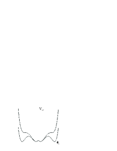
Figure 2: New minima appear in the potential for $um^{2}\neq 0$. The effective potential is shown here for two situations: for $M_{p}^{2}=M_{p}^{c2}$, where the first order transition from LMAF to SMAF occurs and these two states become degenerate and for the spinodal point at which the LMAF becomes unstable inside the SMAF phase.

Now, for many cases of interest, SC fluctuations are better described by a dissipative propagator associated with a $z=2$ dynamics Ramazashvili ; Kirkpatrick similar to Eq. (5). This is useful to account for pair breaking interactions, as magnetic impurities that can destroy superconductivity Sigrist . It is given by,

$$G_{0}(\omega,{\bf q})=\frac{i}{i|\omega|\tau^{\prime}-q^{2}-m^{2}}.$$ (22)

The parameter $m^{2}$ is still related to the distance from the SC phase transition and we have a relaxation time $\tau^{\prime}$. Calculation of the effective potential is very similar to the previous cases and the result has the form

$$V_{eff}=\frac{1}{2}M_{p}^{2}\phi_{3}^{2}+\frac{1}{4!}\tilde{g}\phi_{3}^{4}+\frac{1}{15\pi^{2}}(2u\phi_{3}^{2}+m^{2})^{5/2}$$ (23)

with a renormalized magnetic mass $M_{p}$ and coupling $\tilde{g}$. Quantum corrections can once again produce a weak first order transition. An analysis of the extrema of the effective potential Eq. (23) shows that the transition can be first order depending on the coupling values. The appearance of SMAF phases is not possible in this case.

IV Coupling to local modes

We now study the coupling of antiferromagnetic (AF) fluctuations to local modes in a three dimensional system. This model is useful to describe the QCP of heavy fermions where local modes can coexist with antiferromagnetic fluctuations. The local modes can be either Kondo si or valence fluctuations miyako . The local propagator in Euclidean space is written as

$$G_{L}(\omega)=\frac{1}{m_{L}^{2}+|\omega|/\tau}$$ (24)

where $m_{L}^{2}$ gives the distance to the QCP and $\tau$ is associated with the lifetime of the excitations. For the AF paramagnons, we have

$$G_{p}(\omega,q)=G_{p}(k)=\frac{1}{m_{p}^{2}+q^{2}+|\omega|}$$ (25)

The action is

$$S = \int d^{4}k[G_{p}^{-1}(k)|\psi|^{2}+\frac{g}{12}|\psi|^{4}+G_{L}^{-1}(\omega)|\phi|^{2}$$ (26)

$$+\frac{\lambda}{12}|\phi|^{4}+\frac{u}{2}|\phi|^{2}|\psi|^{2}].$$

Let us consider one component fields, the classical potential (not including the mass terms) is given by,

$$V_{cl}(\phi,\psi)=\frac{g}{12}\psi^{4}+\frac{\lambda}{12}\phi^{4}+\frac{u}{2}\phi^{2}\psi^{2}$$ (27)

and the effective potential by,

$$V^{(1)}(\psi_{c})=\frac{1}{2}\int\frac{d^{4}k}{(2\pi)^{4}}\ln\left(1+\frac{u\psi_{c}^{2}}{m_{L}^{2}+|\omega|/\tau}\right)$$

$$+\frac{1}{2}\int\frac{d^{4}k}{(2\pi)^{4}}\left(1+\frac{g\psi_{c}^{2}}{m_{p}^{2}+q^{2}+|\omega|}\right)+\cdots$$ (28)

where the dots represent counter-terms futuro . The integration in $\omega$ in the first integral can be performed using a cut-off, $\Lambda^{z}-m_{L}^{2}{\tau}$ ($z=2$). However, the integral over $d{\bf q}$ diverges when $\Lambda\rightarrow\infty$ and this term is non-renormalizable unless we introduce a cut-off $q_{c}$ and for later purposes $\tilde{\tau}=(4q_{c}^{3})/(3\pi)$.

IV.1 Case $m_{L}^{2}\gg\tilde{\tau}u^{2}$

In this case the analysis of the renormalized effective potential shows that, as for the classical potential, there is a second order phase transition at $m_{p}^{2}=0$ and the coupling to the local modes has no significant effects.

IV.2 Case $m_{L}^{2}\ll\tilde{\tau}u^{2}$

This is the most interesting case. The renormalized effective potential after dimensional transmutation is given by,

$$V_{eff}(\psi)=\tilde{M}_{p}^{2}\psi^{2}+\tilde{G}\psi^{4}+\frac{\pi^{2}}{(2\pi)^{4}}\left[-\tilde{\tau}u\psi^{2}\ln\left(\frac{\psi^{2}}{\langle\psi\rangle^{2}}\right)\right.$$

$$\left.+\frac{8}{15}\left(-\frac{6m_{p}^{2}\pi^{2}+\tilde{\tau}u}{\langle\psi\rangle^{2}\pi^{2}}\psi^{2}+m_{p}^{2}\right)^{5/2}\!\!\!\!\!\!-\tilde{\tau}m_{L}^{2}\ln(u\psi^{2})\right]$$ (29)

where the renormalized quantities $\tilde{M}_{p}^{2}$ and $\tilde{G}$ are independent of $g$ futuro . In this case we find there is no transition for $m_{p}^{2}\geq 0$, such that, there is no dynamic symmetry breaking. A first order transition occurs for negative values of $m_{p}^{2}$, at a critical value ${m_{p}^{c}}^{2}$ which has to be obtained numerically. The limit of stability of the minima of the effective potential (spinodal) is given by, $m^{2}_{p,sp}=-(\tilde{\tau}u)/(4\pi^{2})$, with $m^{2}_{p,sp}>{m_{p}^{c}}^{2}$. For the particular case $m_{L}^{2}=0$ there is a first order transition between the paramagnetic and antiferromagnetic phases, as shown in Fig. 3. Then, even in $3d$, when both transitions coincide, the magnetic transition becomes first order due to the effect of the critical local fluctuations.

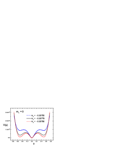
Figure 3: For $m_{L}^{2}=0$ there is a first order transition to the antiferromagnetic phase futuro .

Now, for $m_{L}^{2}$ small but $\neq 0$, the phase diagram changes drastically since new minima appear in the potential close to the origin. These minima which correspond to small values of the order parameter (SMAF) can coexist with those associated with the large values of this parameter (LMAF). As $m_{p}^{2}$ further decreases there is a first order transition between the SMAF and LMAF phases (see fig. 4).

Figure 4: For $m_{L}^{2}\neq 0$ new minima appear close to the origin futuro .

V Scaling at a weak first order quantum transition

At a first order transition there is no true critical behavior since the correlation length does not diverge. However it turned out to be useful to develop a scaling approach for these transitions in the classical case berker . As we show below the same is true for first order quantum phase transitions. This is particularly useful for WFOQPT where we expect the correlation length and characteristic time to become very large. The best way to introduce these ideas is to consider a specific case, for example, the Coleman-Weinberg transition of section II.

Introducing a parameter $g=m^{2}-m_{c}^{2}$ which measures the distance to the first order transition at $m_{c}$, we can write Eq. 3 for the effective potential at $T=0$ and for $g$ small as,

$$V_{eff}=\frac{1}{4}\langle\varphi\rangle^{2}|m^{2}-m_{c}^{2}|\propto|g|^{2-\alpha}$$ (30)

with the exponent $\alpha=1$ reflecting the fact the transition is first order PhysicaA . The associated latent heat is $L_{h}=\frac{1}{4}m_{c}^{2}\langle\varphi\rangle^{2}$. Spinodal points at $T=0$ can also be calculated PhysicaA .

Figure 5: Phase diagram of a charged superfluid coupled to photons. For completeness we show also the critical line of the neutral superfluid. Along the trajectory $m^{2}=m_{c}^{2}$ one can distinguish different regimes as explained in the text.

The finite temperature case can be studied replacing the frequency integrations in the calculation of the effective potential by sums over Matsubara frequencies livro . The effective potential at finite temperatures close to the transition can be written as PhysicaA

$$V_{eff}(T)=\frac{1}{4}m^{2}\langle\varphi\rangle^{2}|g|\left[1\!+\!\frac{2}{\pi^{2}m^{2}\langle\varphi\rangle^{2}}\frac{T^{d+1}}{|g|}I_{d}\!\left(\frac{M(\varphi)}{T}\right)\right]$$

where the integral $I$ is given by

$$I_{d}(y)=\int_{0}^{\infty}dxx^{d-1}\ln{\left[1-e^{-\sqrt{x^{2}+y^{2}}}\right]}.$$ (31)

and $M(\varphi)=m^{2}+q^{2}\varphi^{2}$. The function $I_{3}(y)=I(y)$ can be obtained numerically integrating Eq. (31).

The finite temperature phase diagram is shown in Fig. 5. For completeness we show the critical line of the neutral superfluid, $T_{SF}\propto|m^{2}|^{\psi}$, which is governed by the shift exponent ${\psi}^{-1}=z/(d+z-2)=1/2$ in $d=3$ (see Ref. livro ). The new line of first order transitions is given by $T_{c}\propto\sqrt{m_{c}^{2}-|m^{2}|}$.

We will now consider the system sitting at the new quantum phase transition point, i.e., at $m^{2}=m_{c}^{2}$ and decrease the temperature. For high temperatures, $T\gg m_{c}$, which corresponds to the regime I of Fig. 5, the function $I_{3}(y)$ saturates, $I_{3}(y<0.12)\approx-2.16$. In this case the effective potential,

$$V_{eff}(T)\approx\frac{1}{4}m^{2}\langle\varphi\rangle^{2}|g|\bigg{\{}1-\frac{4.32}{\pi^{2}m^{2}\langle\varphi\rangle^{2}}\frac{T^{d+1}}{|g|}\bigg{\}}$$

and can be cast in the scaling form,

$$V_{eff}(T)\propto|g|^{2-\alpha}F\left[\frac{T}{T_{\times}}\right].$$

with $F(0)=$ $constant$. This scaling form is reminiscent of that for the free energy close to a quantum critical point. In the present case of a discontinuous zero temperature transition, the critical exponent PhysicaA $\alpha=1$ and the characteristic temperature is,

$$T_{\times}\propto|g|^{\nu z}\propto|g|^{\frac{z}{d+z}}=|g|^{\frac{1}{d+1}}=|g|^{\frac{1}{4}}$$

with $\nu=1/(d+z)$ PhysicaA . In this regime I or scaling regime, along the line $m^{2}=m_{c}^{2}$ shown in Fig. 5, the free energy density has therefore the scaling form $f(m=m_{c},T)\propto T^{(d+z)/z}$ and the specific heat is given by,

$$C/T\big{|}_{(m=m_{c},T)}\propto T^{\frac{d-z}{z}}.$$ (32)

Then the thermodynamic behavior along the line $m^{2}=m_{c}^{2}$ in regime I ($T\gg m_{c}$) is the same as when approaching the quantum critical point of the neutral superfluid, along the critical trajectory $m^{2}=0$. The system is unaware of the change in the nature of the zero temperature transition and at such high temperatures charge is irrelevant.

When further decreasing temperature along the line $m^{2}=m_{c}^{2}$ there is an intermediate, non-universal regime (regime II in Figs. 5). In the present case for $T\sim m_{c}$ the specific heat $C/T^{d/z}\propto\ln T$ PhysicaA .

Finally, at very low temperatures, for $T<<m_{c}$ and $m^{2}=m_{c}^{2}$, i.e., in regime III of Fig. 5, the specific heat vanishes exponentially with temperature, $C/T^{d/z}\propto\exp(-m_{c}/T)$. The gap for thermal excitations is given by the shift $m_{c}$ of the quantum phase transition. The correlation length which grows along the line $m^{2}=m_{c}^{2}$ with decreasing temperature reaches saturation in regime III at a value $\xi_{S}$ which is function of the inverse of the gap. The exponential dependence of the specific heat is due to gapped excitations inside superconducting bubbles of finite size $\xi_{S}\propto m_{c}^{-1/z}$.

Although the results above have been obtained for the model of section II, the behavior in the scaling regime I and III should be universal and characteristic of any weak first order quantum transition. Notice that the relevant critical exponents which determine the scaling behavior in particular in regime I are those associated with the QCP of the uncoupled system which in the present case is the neutral superfluid.

- (1) S. Sachdev, Quantum Phase Transitions, CUP, 2000.
- (2) J. A. Hertz, Phys. Rev. B 14, 1165 (1976).
- (3) M. A. Continentino, Quantum Scaling in Many-Body Systems, World Scientific, Singapore, Lecture Notes in Physics - vol. 67 (2001).
- (4) M. A. Continentino, G. Japiassu and A. Troper, Phys. Rev. B 39, 9734, (1989).
- (5) A. J. Millis, Phys. Rev. B 48, 7183 (1993).
- (6) J. Flouquet, Progress in Low Temperature Physics, 15, 139, (Edited by W.P Halperin, Elsevier) (2005) and references therein.
- (7) N. D. Mathur, et al. Nature 394, 39 (1998).
- (8) Q. Si, S. Rabello, K. Ingersent, J. L. Smith, Nature 413, 804 (2001).
- (9) E. Sherman et al., Phys. Rev. Lett. 91 057201 (2003)
- (10) D. Belitz, T.R. Kirkpatrick and T. Vojta, Rev. Mod. Phys. 77, 579 (2005).
- (11) B. I. Halperin, T. Lubensky and S.K. Ma, Phys. Rev. Lett. 32, 292 (1974).
- (12) S. Coleman and E. Weinberg, Phys. Rev. D 7, 1888 (1973).
- (13) M. A. Continentino and A. S. Ferreira, Physica A 339, 461-468 (2004).
- (14) A. S. Ferreira and M. A. Continentino, J. Stat. Mech., P05005 (2005).
- (15) A. S. Ferreira, M. A. Continentino and E. C. Marino, Sol. St. Comm. 130, 321 (2004).
- (16) A. S. Ferreira, M. A. Continentino and E. C. Marino, Phys. Rev. B 70, 174507 (2004).
- (17) R. Ramazashvili and P. Coleman, Phys. Rev. Lett. 79, 3752 (1997)
- (18) T. R. Kirkpatrick and D. Belitz, Phys. Rev. Lett. 79, 3042 (1997).
- (19) V. P. Mineev and M. Sigrist, Phys. Rev. B 63, 172504 (2001).
- (20) A. T. Holmes, D. Jaccard, and K. Miyake Phys. Rev. B 69, 024508 (2004).
- (21) A.S. Ferreira and M.A. Continentino to be submitted.
- (22) M. E. Fisher and A. N. Berker, Phys. Rev. B 026, 2507 (1982).