Non-orthogonal Theory of Polarons and Application to Pyramidal Quantum Dots

Abstract

We present a general theory for semiconductor polarons in the framework of the Fröhlich interaction between electrons and phonons. The latter is investigated using non-commuting phonon creation/annihilation operators associated with a natural set of non-orthogonal modes. This setting proves effective for mathematical simplification and physical interpretation and reveals a nested coupling structure of the Fröhlich interaction. The theory is non-perturbative and well adapted for strong electron-phonon coupling, such as found in quantum dot (QD) structures. For those particular structures we introduce a minimal model that allows the computation and qualitative prediction of the spectrum and geometry of polarons. The model uses a generic non-orthogonal polaron basis, baptized “the natural basis”. Accidental and symmetry-related electronic degeneracies are studied in detail and are shown to generate unentangled zero-shift polarons, which we consistently eliminate. As a practical example, these developments are applied to realistic pyramidal GaAs QDs. The energy spectrum and the 3D-geometry of polarons are computed and analyzed, and prove that realistic pyramidal QDs clearly fall in the regime of strong coupling. Further investigation reveals an unexpected substructure of “weakly coupled strong coupling regimes”, a concept originating from overlap considerations. Using Bennett’s entanglement measure, we finally propose a heuristic quantification of the coupling strength in QDs.

I Introduction

Quantum structures (QSs), such as quantum dots (QDs), are sophisticated solid-state pieces, vital for fundamental research and novel applications in quantum optics and quantum informatics. Today, QDs find technological use in QD lasers,Huffaker 03 infrared photodetectors,Lee 99 single photon sources Santori 01 ; Pelton 02 or markers in biology.Mingyong 01 Cutting-edge research features QDs as medical fluorophores for in vivo detection of cell structures such as tumors.Xingyong 02 Other promising applications for QDs are solar cells Schaller 04 and optical telecommunication.Klopf 01 The most exciting, yet challenging expectation relies in the use of QDs as qubit holders and gates for quantum computation.Loss 98 For fundamental science, QDs are among the few systems allowing controlled experiments with single energy quanta giving direct access to controlled quantum entanglement and correlations.

Due to their extreme carrier sensitivity, much interest in QDs relates to carrier relaxation and excitation processes mediated by various interactions, such as carrier-carrier, carrier-photon and carrier-phonon interactions. As for carrier-phonon interactions, early perturbative approaches with acoustic phonons resulted in the bottleneck concept.Bockelmann 90 ; Benisty 91 ; Brunner 92 ; Bockelmann 93 Theses perturbative results predict inefficient carrier relaxation for a large class of small QDs. Although experimentally verified in certain cases Urayama 01 ; Heitz 01 , these predictions failed in many other tests.Notomi 91 ; Raymond 95 A definite progress came with non-perturbative investigations of the deformation potential and Fröhlich interaction, revealing the existence of a strong coupling regime, which is out of reach of perturbative approaches and allows efficient carrier relaxation through acoustic and optical phonon dynamics respectively.Inoshita 97 ; Kral 98 ; Hameau 99 ; Verzelen 00 This led to the new concept of quantum dot polarons (QDPs), which are non-separable fundamental excitations determined by the carrier-phonon interaction. Within the approximation of monochromatic LO-modes for the Fröhlich interaction, electrons only couple to a finite number of lattice modes as analytically explained through an algebraic decomposition introduced by Stauber et al.Stauber 00 Their procedure constructs an orthonormalized basis of relevant lattice modes from the finite set of phonon creation/annihilation operators naturally appearing in the Fröhlich Hamiltonian. This leads to a numerically solvable model of QDPs Stauber 06 , which can be viewed as an extension of the work by Ferreira et al.Ferreira 03

In this work, the polaron problem is tackled from a different viewpoint: the full electron-phonon Hamiltonian is reformulated in terms of non-orthogonal modes, which naturally span all coupled and uncoupled crystal vibrations. The non-orthogonal structure is preserved from the beginning to the end and exhibits undisputable advantages for computation and physical understanding. General analytical results applicable to any type of semiconductor QS are derived in this framework. They are subsequently applied to peculiar pyramidal $C_{3v}$ GaAs QDs, but the same theoretical scheme could be applied to any other semiconductor QD structure, e.g. zincblende $InAs$ QDs with $C_{2v}$ symmetryGammon 96 or Wurzite $GaN$ QDs with high $C_{3v}$ or $C_{6v}$ symmetry.Tronc 04

Section II considers a general QS populated by an arbitrary number of bound electrons and phonons. We first introduce a set of non-orthogonal LO-modes, which spans all the LO-modes appearing in the Fröhlich interaction. From there we derive two decoupled subalgebras of non-commuting phonon creation/annihilation operators, which separate the quantum structure in a subsystem of bound polarons and a subsystem of uncoupled modes (II.2). The theory culminates in a non-trivial nested coupling structure of the Fröhlich interaction, which has important consequences when working with any finite number of phonons (II.3). In section III, we introduce a minimal non-perturbative model (one electron, one phonon) particularly suitable for the crucial case of QDPs. We provide an explicit non-orthogonal polaron basis, baptized the “natural basis” (III.1). It provides a detailed interpretation of the geometries and spectra of low-energy QDPs. We also investigate additional simplifications resulting from electronic degeneracies (III.2) and group theoretical considerations of dot symmetries (III.3). The theory concludes with some key aspects of the three-dimensional (3D) numerical code (III.4), which comprises an adaptive irregular space discretization for computing the Fröhlich matrix elements.

In a second part, the minimal model is applied to realistic pyramidal GaAs QDs with $C_{3v}$ symmetry. Kapon 04 Section IV presents the 3D-geometries of the QDPs and their spectrum, throughout using group theory (IV.1, IV.2, IV.5). Explicit comparison with perturbation theory confirms the existence of a strong coupling regime. Surprisingly, we find significant numerical evidence for a peculiar substructure inside the strong coupling regime. This leads to the concept of “weakly coupled strong coupling regimes” (IV.3), which can be understood in terms of overlap between confined electrons and coupled modes. Using Bennett’s entanglement measure, we further present a useful alternative characterization of the strong electron-phonon coupling in QDs (IV.4).

In section V, we report on the general polaron properties that could be expected in other QD systems. Section  VI concludes the theory with a short review, and helpful derivations are provided in the appendix VII.

II Non-orthogonal theory for polaron states

In this section, we present a theory for polar semiconductor QSs, e.g. dots, wires or wells, in which the carrier evolution is reasonably described by Fröhlich interactions with monochromatic LO-modes. The QSs can contain an arbitrary number of electrons (within the limitations induced by the Pauli exclusion principle) and an arbitrary number of phonons. The conservation laws exhibited by the interaction Hamiltonian allow straightforward generalizations to exciton-polarons or even polarons associated with bigger electron/hole complexes.

II.1 Polaron Hamiltonian in Quantum Structures

The model’s evolution is dictated by a Hamiltonian composed of a free evolution term and the Fröhlich Hamiltonian $H^{int}$,

$$\begin{split}\hbox to0.0pt{$\displaystyle H$\hss}\qquad&=\sum_{\mu\,\sigma}\epsilon_{\mu}a_{\mu\sigma}^{\dagger}a_{\mu\sigma}+\epsilon_{LO}\sum_{\mathbf{q}}b_{\mathbf{q}}^{\dagger}b_{\mathbf{q}}+H^{int}\\ \@ADDCLASS{ltx_eqn_lefteqn}$\displaystyle H^{int}$\mbox{}\hfil\qquad&=\sum_{\mu\mu^{\prime}\sigma\mathbf{q}}M_{\mu\mu^{\prime}\mathbf{q}}a_{\mu\sigma}^{\dagger}a_{\mu^{\prime}\sigma}b_{\mathbf{q}}+h.c.\\ \end{split}$$ (1)

(Unity operators and tensor products have been omitted.) $a_{\mu\sigma}$, $a_{\mu\sigma}^{\dagger}$ are fermionic annihilation and creation operators of confined conduction electrons, with $\mu$ labeling an orthogonal set of stationary wave functions and $\sigma$ being the spin index. The scalars $\epsilon_{\mu}$ are the free electronic energies, which are independent of $\sigma$ in the absence of magnetic fields. $b_{\mathbf{q}}$, $b^{\dagger}_{\mathbf{q}}$ are the bosonic annihilation and creation operators of phonons associated with the LO-plane waves $\xi_{\mathbf{q}}(\mathbf{x})\equiv\sqrt{2/V}e^{i\mathbf{q}\cdot\mathbf{x}}$, where $V$ is the quantization volume. $\epsilon_{LO}=\hbar\omega_{LO}$ is the phonon energy assumed independent of $\mathbf{q}$ (monochromaticity), and $M_{\mu\mu^{\prime}\mathbf{q}}$ are the Fröhlich matrix elements Froehlich 49

$$\begin{split}M_{\mu\mu^{\prime}\mathbf{q}}=&\sqrt{\frac{\hbar\omega_{LO}e^{2}}{2\varepsilon_{0}Vq^{2}}\left(\frac{1}{\varepsilon_{\infty}}-\frac{1}{\varepsilon_{stat}}\right)}\\ &\times\ \int_{\mathbb{R}^{3}}d^{3}x\ e^{i\mathbf{q}\cdot\mathbf{x}}\psi_{\mu}^{\ast}(\mathbf{x})\psi_{\mu^{\prime}}(\mathbf{x})\\ \end{split}$$ (2)

where $\varepsilon_{stat}$ and $\varepsilon_{\infty}$ are the static and high frequency dielectric constants and $\psi_{\mu}(\mathbf{x})$ are the (one-particle) electronic wave functions. Since the Hamiltonian (1) is decoupled and symmetrical in spin degrees of freedom, we shall from here on omit the spin indices $\sigma$.

II.2 Subsystem of Quantum Structure Polarons

We shall now apply a non-orthogonal linear transformation to the operator basis $\{b_{\mathbf{q}},b^{\dagger}_{\mathbf{q}}\}$ in order to reveal two decoupled physical subsystems, the subsystem of “Quantum Structure Polarons” (QSPs) and the subsystem of “Uncoupled Phonons” (Uphs). This conceptual separation will be reflected in a tensor product decomposition of the representative Hilbert space.

The matrix elements (2) can be considered as discrete 3-dimensional functions of $\mathbf{q}$. They obey relations of linear dependance, as can be seen by choosing the electronic wave functions $\psi_{\mu}(x)$ real (always possible), in which case $M_{\mu\mu^{\prime}\mathbf{q}}=M_{\mu^{\prime}\mu\mathbf{q}}$. If there are $N$ orthogonal electron states $\mu$, the number of such relations is $N(N-1)/2$. The remaining $N(N+1)/2$ matrix elements show no obvious relations of linear dependance, and we shall temporarily assume that there are the only $N(N-1)/2$ independent relations of linear dependance. The theory remains valid in the case of additional linear dependencies such as discussed towards the end of this subsection.

The structure of the Fröhlich interaction implies that the number of linearly independent matrix elements $M_{\mu\mu^{\prime}\mathbf{q}}$ equals the number of linearly independent lattice modes that appear in the interaction term. This can be seen explicitly, when reformulating the interaction as

$$H^{int}$$    = ∑_μμ’ J_μμ’ a_μ^†a_μ’ B_μμ’ + h.c. (3)

$$B_{\mu\mu^{\prime}}$$    ≡ 1Jμμ’ ∑_qM_μμ’q b_q≡∑_qL_μμ’q b_q (4)

where $|J_{\mu\mu^{\prime}}|^{2}=\sum_{\mathbf{q}}|M_{\mu\mu^{\prime}\mathbf{q}}|^{2}$ quantizes the electron-phonon coupling strength, with $J_{\mu\mu^{\prime}}$ chosen as a positive real. The relations of linear dependance among the matrix elements $M_{\mu\mu^{\prime}\mathbf{q}}$ trivially translate to $B^{{\dagger}}_{\mu\mu^{\prime}}=B^{{\dagger}}_{\mu^{\prime}\mu}$ and $B_{\mu\mu^{\prime}}=B_{\mu^{\prime}\mu}$. The remaining $N(N+1)/2$ linearly independent phonon operators shall be scanned by a unique pair index $\lambda\equiv\{\mu,\mu^{\prime}\}=\{\mu^{\prime},\mu\}$.

The operators $\{B_{\lambda},B^{{\dagger}}_{\lambda}\}$ annihilate and create “coupled phonons”, that is quanta in terms of a harmonic oscillator in modes susceptible to interact with electrons via the Fröhlich potential. Using (4), the wave functions of those modes are given by the inverse Fourier transforms

$$\Xi_{\lambda}(\mathbf{x})=\sum_{q}L^{\ast}_{\lambda\mathbf{q}}\xi_{q}(\mathbf{x})\equiv\sqrt{\frac{2}{V}}\sum_{q}e^{i\mathbf{q}\cdot\mathbf{x}}L^{\ast}_{\lambda\mathbf{q}}$$ (5)

which are manifestly localized in the quantum structure. The set of all modes $\Xi_{\lambda}(\mathbf{x})$ is non-orthogonal as emphasized by the non-diagonal scalar product matrix and the non-diagonal commutator of the corresponding operators $\{B_{\lambda},B^{{\dagger}}_{\lambda}\}$. Both follow directly from (5) and (4),

$$\Lambda_{\lambda\lambda^{\prime}}\equiv\left[B_{\lambda},B^{\dagger}_{\lambda^{\prime}}\right]=\big{(}\Xi_{\lambda},{\Xi_{\lambda^{\prime}}}\big{)}=\sum_{\mathbf{q}}L^{\ast}_{\lambda^{\prime}\mathbf{q}}L_{\lambda\mathbf{q}}$$ (6)

(Round brackets represent the scalar product relative to the quantization volume $V$.) For reasons of physical interpretation and mathematical simplicity, we skip a possible orthonormalization and preserve the non-orthogonality for the rest of the theory.

In order to express the full Hamiltonian in terms of the new operators $\{B^{{\dagger}}_{\lambda},B_{\lambda}\}$, we need to complete them by an operator-set $\{B^{{\dagger}}_{\mathbf{q}},B_{\mathbf{q}}\}$ generating the orthogonal complement $\{\Xi_{\mathbf{q}}(\mathbf{x})\}$ of the coupled modes $\{\Xi_{\lambda}(\mathbf{x})\}$. We choose a linear transformation,

$$B_{\mathbf{q}}^{\dagger}\equiv\sum_{\mathbf{q}^{\prime}}{c_{\mathbf{q}\mathbf{q}^{\prime}}{b_{\mathbf{q}^{\prime}}}^{\dagger}}\ ,\,\ \ \Xi_{\mathbf{q}}(\mathbf{x})\equiv\sum_{\mathbf{q}^{\prime}}{c_{\mathbf{q}\mathbf{q}^{\prime}}\xi_{\mathbf{q}}(\mathbf{x})}$$ (7)

A natural and sufficient condition for the coefficients $c_{\mathbf{q}\mathbf{q}^{\prime}}$ writes $B_{\mathbf{q}}^{\dagger}\big{|}0\big{>}=(\openone_{1\,ph}-\mathcal{P})\,b_{\mathbf{q}}^{\dagger}\big{|}0\big{>}$, where $\big{|}0\big{>}$ is the phonon vacuum, $\openone_{1\,ph}$ the unity on the subspace of one phonon, and $\mathcal{P}$ is the orthogonal projector on the sub-subspace of coupled one-phonon states $vect\{B_{\lambda}^{\dagger}\big{|}0\big{>}\}$. Thus $(\openone_{1\,ph}-\mathcal{P})$ projects on the one-phonon sub-subspace of uncoupled modes, and $\{B^{{\dagger}}_{\mathbf{q}}\}$ creates quanta accordingly called “uncoupled phonons”. An explicit derivation of the coefficients $c_{\mathbf{q}\mathbf{q}^{\prime}}$ is provided in appendix VII.1. From this explicit form it follows that the modes $\{\Xi_{\mathbf{q}}(x)\}$ are also mutually non-orthogonal, which again translates to a non-diagonal commutator of the corresponding creation/annihilation operators $\{B_{\mathbf{q}}^{\dagger},B_{\mathbf{q}}\}$,

$$\left[B_{\mathbf{q}},B^{{\dagger}}_{\mathbf{q}^{\prime}}\right]=\big{(}\Xi_{\mathbf{q}},{\Xi_{\mathbf{q}^{\prime}}}\big{)}=\sum_{q^{\prime\prime}}{c^{\ast}_{\mathbf{q}\mathbf{q}^{\prime\prime}}c_{\mathbf{q}^{\prime}\mathbf{q}^{\prime\prime}}},$$ (8)

Indeed, the modes $\{\Xi_{\mathbf{q}}(x)\}$ constitute an overcomplete set, according to the $N(N+1)/2$ relations of linear dependence

$$\sum_{\mathbf{q}}L^{\ast}_{\lambda\mathbf{q}}B^{\dagger}_{\mathbf{q}}=\sum_{\mathbf{q}}L^{\ast}_{\lambda\mathbf{q}}\Xi_{\mathbf{q}}(\mathbf{x})=0\ \ \forall\lambda$$ (9)

However, it is important to note that all coupled modes $\{\Xi_{\lambda}(\mathbf{x})\}$ are orthogonal to all uncoupled ones $\{\Xi_{\mathbf{q}}(\mathbf{x})\}$, as emphasized by the following commutators and scalar products

$$\left[B_{\lambda},B^{{\dagger}}_{\mathbf{q}}\right]=\big{(}\Xi_{\lambda},\Xi_{\mathbf{q}}\big{)}=0$$ (10)

The transformations (4) and (7) constitute a non-orthogonal mapping $\{b_{\mathbf{q}}^{\dagger}\}\rightarrow\{B_{\lambda}^{\dagger},B_{\mathbf{q}}^{\dagger}\}$. The inversion $\{b_{\mathbf{q}}^{\dagger}\}\leftarrow\{B_{\lambda}^{\dagger},B_{\mathbf{q}}^{\dagger}\}$ is not unique due to the overcompleteness of $\{B_{\mathbf{q}}^{\dagger}\}$. A suitable form, consistent with (4) and (7), is given by

$$b^{\dagger}_{\mathbf{q}}=B^{\dagger}_{\mathbf{q}}+\sum_{\lambda\lambda^{\prime}}L_{\lambda^{\prime}\mathbf{q}}(\Lambda^{-1})_{\lambda\lambda^{\prime}}B^{\dagger}_{\lambda}$$ (11)

This allows us to express the phonon number operator in terms of the new operators,

$$\sum_{\mathbf{q}}b_{\mathbf{q}}^{\dagger}b_{\mathbf{q}}=\sum_{\lambda\lambda^{\prime}}\big{(}\Lambda^{-1}\big{)}_{\lambda\lambda^{\prime}}B_{\lambda}^{\dagger}B_{\lambda^{\prime}}+\sum_{\mathbf{q}}B_{\mathbf{q}}^{\dagger}B_{\mathbf{q}}$$ (12)

Finally, the full Hamiltonian (1) transforms to

$$H$$ = H^QSP+H^Uph, H^QSP≡H^0+H^int (13)

$$H^{0}$$ ≡ ∑_μϵ_μa_μ^†a_μ+ ϵ_LO∑_λλ’ (Λ^-1)_λλ’B_λ^†B_λ’ (14)

$$H^{Uph}$$ ≡ ϵ_LO∑_q B_q^†B_q (15)

(unity operators and tensor products have been omitted). The fundamental commutators (10) imply the commutator

$$\left[H^{QSP},H^{Uph}\right]=0$$ (16)

The latter defines a unique separation in two physical subsystems, expressed by the tensor product decomposition

$$\mathcal{H}=\mathcal{H}^{QSP}\otimes\mathcal{H}^{Uph}$$ (17)

such that $H^{QSP}$ acts trivially in $\mathcal{H}^{Uph}$ and $H^{Uph}$ acts trivially in $\mathcal{H}^{QSP}$. [(17) assumes the bosonic symmetrization of the phonon subsystem.] The subsystem represented in $\mathcal{H}^{QSP}$ consists of electrons and coupled phonons associated with a finite number of $N(N+1)/2$ linearly independent modes $\{\Xi_{\lambda}(\mathbf{x})\}$. The stationary states (i.e. eigenstates of $H^{QSP}$) are likely entangled in electronic and phononic coordinates and will be referred as to “quantum structure polarons” (QSPs). In contrast, the subsystem of “uncoupled phonons”, represented in $\mathcal{H}^{Uph}$, is a pure phonon-system associated with infinitely many uncoupled bulk modes $\{\Xi_{\mathbf{q}}(\mathbf{x})\}$. Each such mode evolves trivially under the phonon number operator, and thus the quantum structure problem drastically reduces to solving $H^{QSP}$ inside $\mathcal{H}^{QSP}$.

This theory remains valid if the Fröhlich matrix elements exhibit other linear dependencies than $M_{\mu\mu^{\prime}\mathbf{q}}=M_{\mu^{\prime}\mu\mathbf{q}}$ (and their linear combinations). Indeed, if there are $N^{\prime}$ linearly independent matrix elements, $N^{\prime}<N(N+1)/2$, it suffices to redefine the index $\lambda$ such as to label only the corresponding independent operators $B_{\mu,\mu^{\prime}}$. The derivation above stays valid with this redefinition, if any number $N(N+1)/2$ is replaced by $N^{\prime}$. (e.g. the number of linear dependencies among the uncoupled modes $B_{q}$ will be reduced to $N^{\prime}$, etc.)

It is worth noting that the Hamiltonian $H^{QSP}$ manifestly conserves the number of electrons, i.e.

$$\Big{[}H^{QSP},\sum_{\mu}\epsilon_{\mu}a_{\mu}^{\dagger}a_{\mu}\Big{]}=0$$ (18)

This conservation law implies the existence of one coupled mode that only couples to the electron number operator, such as shown by Stauber et al. Stauber 06 In contrast to their choice, we decide to keep this particular mode in the system of QSPs. Indeed, even though this mode does not affect the overall electron dynamics, it is located in the quantum structure and evolves through the creation an reannihilation of intermediate electrons. Therefore, its stationary solutions are Glauber-coherent states, very different from the stationary phonon-number states of uncoupled modes.

II.3 Nested Coupling Structure

In this section, we shall uncover a nested structure in the Fröhlich coupling. This structure implies in particular that certain states differing by one phonon (e.g. a state with one phonon and a state with two phonons) are exclusively coupled via intermediate higher order states (e.g. a state with three phonons). This non-trivial coupling structure provides some intuition for the form of stationary states and implies a rule to truncate the Hilbert space if the polaron problem is restricted to a finite number of phonons.

In the following non-perturbative analysis, two states $\big{|}\psi\big{>},\big{|}\varphi\big{>}$ are called “coupled” if the evolution of one state develops a non-vanishing projection on the other, i.e. $\big{<}\psi\big{|}exp(-iH^{QSP}t)\big{|}\varphi\big{>}\neq 0$ for at least one $t$. Thus the subspace $\mathcal{H}_{a}$ coupled to a subspace $\mathcal{H}_{b}$ is given by

$$\mathcal{H}_{a}=vect\left\{e^{-iH^{QSP}t}\big{|}\varphi\big{>}\ :\forall\,t,\big{|}\varphi\big{>}\in\mathcal{H}_{b}\right\}$$ (19)

In order to identify a coupling structure, we first use the conservation of the number of electrons [eq. (18)]. It reveals that coupling structure can be identified individually for each fixed number of electrons without loss of generality. For the rest of this section, we shall thus restrict our considerations to some fixed number of electrons $m$ ($m\geq 1$), and take the subspace $\mathcal{H}^{QSP}$ as restricted to $m$ electrons. Second, we note that $H^{QSP}$ does not couple orthogonal spin states, and hence the coupling structure can be investigated with all electrons having the same fixed spin $\sigma$. As $H^{QSP}$ acts identically on all values of $\sigma$ spins can be generally neglected (as in the previous section). Third, we use the property that the Fröhlich operator $H^{int}$ affects phonon numbers by one unit. Hence, it is useful to decompose $\mathcal{H}^{QSP}$ in subspaces associated with different numbers of phonons $k$,

$$\begin{split}\mathcal{H}^{QSP}&=\bigoplus_{k=0}^{\infty}\mathcal{H}^{QSP}_{k}\\ \mathcal{H}^{QSP}_{k}&\equiv vect\Big{\{}a^{\dagger}_{\nu_{1}}\cdots a^{\dagger}_{\nu_{m}}B^{\dagger}_{\mu_{1}\mu^{\prime}_{1}}\cdots B^{\dagger}_{\mu_{k}\mu^{\prime}_{k}}\big{|}0\big{>}\Big{\}}\\ \end{split}$$ (20)

The index list $\{\nu_{i},\mu_{i},\mu^{\prime}_{i}\}$ goes over all combinations of electronic indices, such that $\nu_{i}\neq\nu_{j}\ \forall\,i\neq j$ (Pauli exclusion principle). Here, $\big{|}0\big{>}\equiv\big{|}0_{electrons}\big{>}\otimes\big{|}0_{phonons}\big{>}$ denotes the polaron vacuum.

According to the coupling rule (19), the subspace coupled to $\mathcal{H}^{QSP}_{k}$ is given by

$$vect\left\{e^{-iH^{QSP}t}\big{|}\varphi\big{>}\ :\forall\,t,\big{|}\varphi\big{>}\in\mathcal{H}^{QSP}_{k}\right\}$$ (21)

To pinpoint a particularity in the coupling between $\mathcal{H}^{QSP}_{p}$ and its “inferior neighbor” $\mathcal{H}^{QSP}_{p-1}$, we shall temporarily restrict the phonon Fock space to at most $p$ phonons ($p>0$). This implicitly requires a truncation of the Hamiltonian $H^{QSP}$ equivalent to imposing $B^{\dagger}_{\lambda}\big{|}\varphi\big{>}=0\ \forall\ \big{|}\varphi\big{>}\in\mathcal{H}^{QSP}_{p}$. We define $\tilde{\mathcal{H}}^{QSP}_{p}$ as the sub-subspace of $\mathcal{H}^{QSP}_{p}$ coupled to $\mathcal{H}^{QSP}_{p-1}$ within this restriction. Departing from (21) with $k=p-1$, $\tilde{\mathcal{H}}^{QSP}_{p}$ can be simplified to (derivation in appendix VII.2)

$$\tilde{\mathcal{H}}^{QSP}_{p}\equiv vect\left\{e^{-iH^{0}t}H^{int}_{+}\big{|}\varphi\big{>}\,:\forall\,t,\big{|}\varphi\big{>}\in\mathcal{H}^{QSP}_{p-1}\right\}$$ (22)

where $H^{0}$ is the free evolution (14) and $H^{int}_{+}\equiv\sum_{\mu\mu^{\prime}}J_{\mu\mu^{\prime}}a_{\mu}^{\dagger}a_{\mu^{\prime}}B^{\dagger}_{\mu\mu^{\prime}}$ denotes the phonon creating part of the Fröhlich interaction (3). In physical terms, (22) expresses that an electron-phonon state $\big{|}\varphi\big{>}$, initially containing $p-1$ phonons, evolves towards a superposition involving a certain $p$-phonon state (by Fröhlich interaction). The latter is generally not an eigenstate of $H^{0}$ and its free evolution can span a whole $p$-phonon subspace coupled to the initial state $\big{|}\varphi\big{>}$. For further simplification we decompose $H^{int}_{+}\big{|}\varphi\big{>}$ in eigenstates of $H^{0}$,

$$H^{int}_{+}\big{|}\varphi\big{>}=\sum_{\gamma}{\mathcal{P}_{\gamma}H^{int}_{+}\big{|}\varphi\big{>}}$$ (23)

where $\gamma$ labels the eigenspaces of $H^{0}$ inside $\mathcal{H}^{QSP}_{p}$, and $\mathcal{P}_{\gamma}$ are the orthogonal projectors on all these eigenspaces. As $\mathcal{P}_{\gamma}$ projects on a $p$-phonon subspace and $\big{|}\varphi\big{>}$ is a $(p-1)$-phonon state, we can safely replace $\mathcal{P}_{\gamma}H^{int}_{+}$ by $\mathcal{P}_{\gamma}H^{int}$, for $\mathcal{P}_{\gamma}$ annihilates the phonon annihilating part of the interaction $H^{int}$. Invoking the relation $e^{-iH^{0}t}\mathcal{P}_{\gamma}H^{int}\big{|}\varphi\big{>}=e^{-i\epsilon_{\gamma}t/\hbar}\mathcal{P}_{\gamma}H^{int}\big{|}\varphi\big{>}$ and substituting (23) in (22) gives

$$\tilde{\mathcal{H}}^{QSP}_{p}=vect\left\{\mathcal{P}_{\gamma}H^{int}\big{|}\varphi\big{>}\,:\forall\,\gamma,\big{|}\varphi\big{>}\in\mathcal{H}^{QSP}_{p-1}\right\}$$ (24)

(since $e^{-i\epsilon_{\gamma}t/\hbar}$ for different $\gamma$ are linearly independent functions of $t$.)

The eigenspace projectors $\mathcal{P}_{\gamma}$ act trivially on the subsystem of lattice modes populated by $p$ phonons, since all $p$-phonon states are degenerate (monochromaticity assumption). As for the electron subsystem (here considered as non-degenerate), the different eigenspaces can be labeled as $\gamma\equiv\{\nu_{1},\ldots,\nu_{m}\}$, where $\{\ldots\}$ denotes an unordered set and $\nu_{i}\neq\nu_{j}\ \forall\,i\neq j$. (Spin indices were omitted according to the introduction of this section.) The electronic part of the projectors $\mathcal{P}_{\gamma}$ can then be expressed as

$$a_{\nu_{1}}^{\dagger}\cdots a_{\nu_{m}}^{\dagger}\big{|}0_{electrons}\big{>}\big{<}0_{electrons}\big{|}a_{\nu_{m}}\cdots a_{\nu_{1}}$$ (25)

Substituting this expression in (24), allows to express $\tilde{\mathcal{H}}^{QSP}_{p}$ with explicit basis vectors. After rearrangement and substitution of indices, we find

$$\tilde{\mathcal{H}}^{QSP}_{p}=vect\Big{\{}a^{\dagger}_{\nu_{1}}\cdots a^{\dagger}_{\nu_{m}}B^{\dagger}_{\mu_{1}\mu^{\prime}_{1}}\cdots B^{\dagger}_{\mu_{p}\mu^{\prime}_{p}}\big{|}0\big{>}\Big{\}}$$ (26)

where $\mu_{1}=\nu_{1}$, and $\mu^{\prime}_{1}\neq\nu_{i}\ \forall i=2,\ldots,m$. Expression (26) shows that $\tilde{\mathcal{H}}^{QSP}_{p}$ is necessarily a subspace of $\mathcal{H}^{QSP}_{p}$.

We conclude that if the number of phonons is limited to $p$ ($p\geq 1$), the subspace $\mathcal{H}^{QSP}_{p-1}$ couples to $\tilde{\mathcal{H}}^{QSP}_{p}$, but not to its orthogonal complement $\tilde{\mathcal{H}}^{QSP\,\perp}_{p}\subset\mathcal{H}^{QSP}_{p}$.

In conclusion, if for physical or computational reasons the model is truncated to a finite number of phonons $p$, then the subspace $\mathcal{H}^{QSP}_{p}$ must be restricted to $\tilde{\mathcal{H}}^{QSP}_{p}$. Otherwise non-physical polarons would appear (contained in $\tilde{\mathcal{H}}^{QSP\,\perp}_{p}$), that would seem uncoupled and thus unshifted relative to the free spectrum. Such a precaution was apparently not taken in previous works.Stauber 06 The particular truncation $\mathcal{H}^{QSP}_{p}\rightarrow\tilde{\mathcal{H}}^{QSP}_{p}$ also represents an analytical and computational simplification.

If we release the temporary assumption of a finite phonon number $p$ (or if we take $k<p$), the following statement holds: $k$-phonon states in $\tilde{\mathcal{H}}^{QSP\,\perp}_{k}$ do not directly couple to $(k-1)$-phonon states, but can only couple to $(k-1)$-phonon states via intermediate $(k+1)$-phonon (and higher order) states! In a perturbative approach, these particular couplings would first appear in the third order of the interaction term. Direct couplings, i.e. couplings that do not involve intermediate higher-order states, are represented by the arrows in Fig. 1. This nested structure provides some insight in the form of stationary polarons (which generally superpose states with different phonon numbers). For example, stationary superpositions of states from $\tilde{\mathcal{H}}^{QSP\,\perp}_{k}$ and $\mathcal{H}^{QSP}_{k-1}$ necessarily involve a strong contribution of states from $\tilde{\mathcal{H}}^{QSP}_{k+1}$. On the other hand, there may be stationary polarons made of states from $\tilde{\mathcal{H}}^{QSP}_{k}$ and $\mathcal{H}^{QSP}_{k-1}$ with only a minor contribution of states from $\mathcal{H}^{QSP}_{k+1}$.

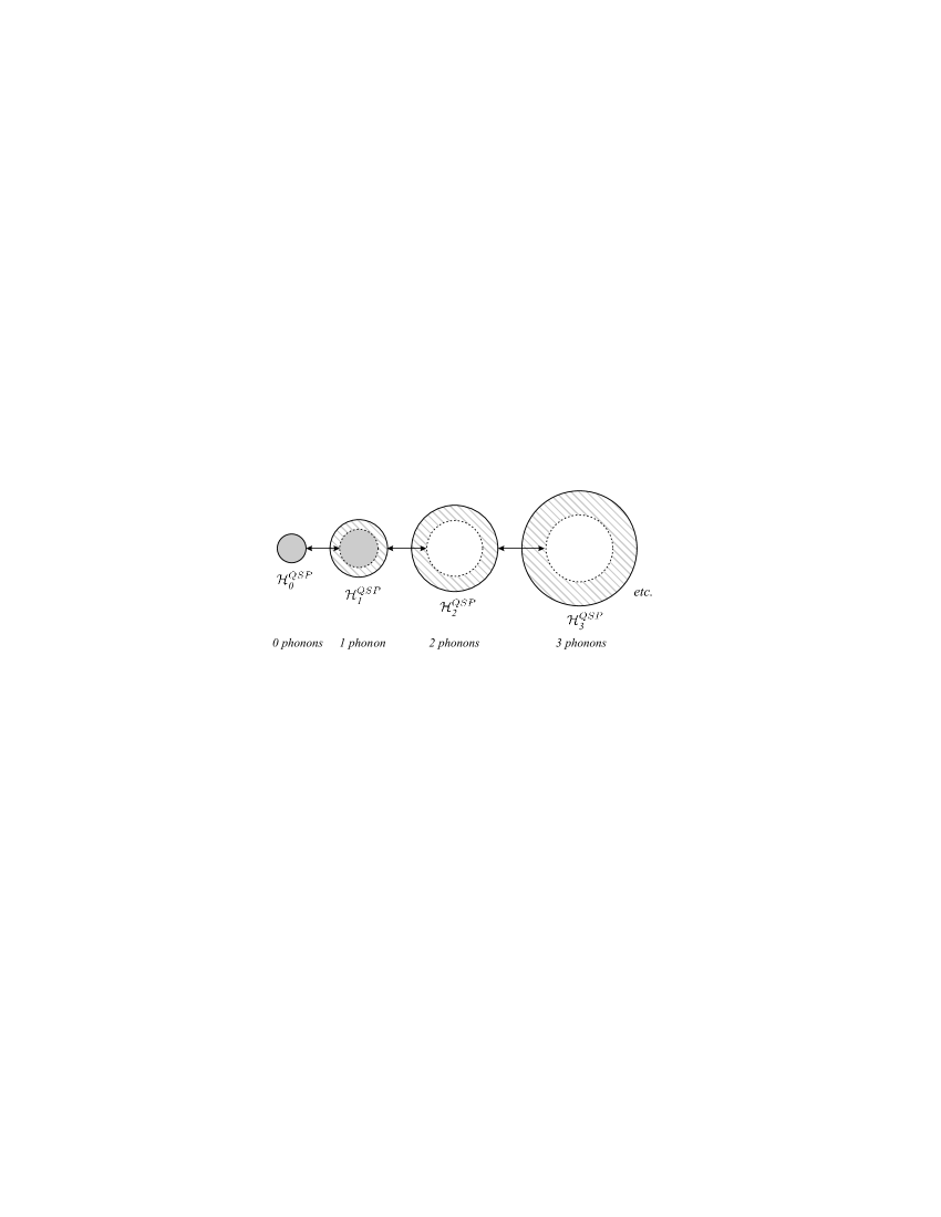
Figure 1: Nested coupling structure exhibited by the Fröhlich interaction. Arrows represent couplings that do not involve intermediate states with a higher number of phonons (see text). Solid circles contain the subspaces $\mathcal{H}^{QSP}_{k}$ for different $k$’s. Dashed circles enclose the subspaces $\tilde{\mathcal{H}}^{QSP}_{k}$, whereas hatched zones show their orthogonal complements $\tilde{\mathcal{H}}^{QSP\,\perp}_{k}$ within $\mathcal{H}^{QSP}_{k}$. The solid gray filling indicates the subspace $\mathcal{H}^{\ast}$ spanned by the natural basis (28).

III One-electron/One-phonon Model of QDPs

In the framework of the general non-orthogonal theory developed above, we shall now propose a minimal non-perturbative model for polaron states in quantum dots (QDs). The general quantum structure considered so far, is now specified as a quantum dot: QS$\rightarrow$QD and QSP$\rightarrow$QDP. In such zero-dimensional systems, the monochromaticity assumption, crucial for the present theory, is fairly precise for the relevant modes (i.e. wavelengths comparable to the dot size and thus long compared to the atomic spacing). The model assumes a single electron ($m=1$) populating different levels while coupling to at most one phonon ($p=1$). It allows to approximate the shifts of the first polaron levels, which are typically populated at low temperatures, although there may be additional effects arising from acoustic phonons like dephasing effects.

In the next three subsections, we subsequently investigate QDs with non-degenerate electron levels (III.1), with accidental degeneracies (III.2), and with symmetry-related degeneracies (III.3). For each case, we develop a simple non-orthogonal polaron-basis $\mathcal{B}^{\ast}$, baptized the “natural basis”, which spans the relevant Hilbert space $\mathcal{H}^{\ast}$. A similar formalism could be developed for holes (although acoustic phonons may have to be taken into account there), or for any many-particle complex such as an exciton-, a trion- or a biexciton-based quantum dot polaron. Stauber and Zimmermann Stauber 06 showed that a correction term must be introduced in the case of non-neutral complexes.

III.1 Natural Basis

We first consider a non-symmetric QD with $N$ non-degenerate electron levels $\mu$. Accordingly there are $N(N+1)/2$ linearly independent coupled modes, spanned by the operators $B^{{\dagger}}_{\mu\mu^{\prime}}$. By virtue of the coupling structure developed in section II.3, the coupled regime of the one-phonon model is properly represented by the subspace $\mathcal{H}^{\ast}$ corresponding to gray filling in Fig. 1. It writes

$$\mathcal{H}^{\ast}\equiv\mathcal{H}^{QDP}_{0}\oplus\tilde{\mathcal{H}}^{QDP}_{1}$$ (27)

A vector set $\mathcal{B}^{\ast}$, such that $\mathcal{H}^{\ast}=vect\,\mathcal{B}^{\ast}$ is directly obtained from (26),

$$\small\mathcal{B}^{\ast}=\Big{\{}\big{|}\mu;0\big{>},B^{\dagger}_{\mu\mu^{\prime}}\big{|}\mu;0\big{>}\equiv\sum_{q}M^{\ast}_{\mu\mu^{\prime}\mathbf{q}}\big{|}\mu;\mathbf{q}\big{>}\ \forall\,\mu,\mu^{\prime}\Big{\}}$$ (28)

where we used the short hands $\big{|}\mu;0\big{>}\equiv a^{\dagger}_{\mu}\big{|}0\big{>}$ and $\big{|}\mu;\mathbf{q}\big{>}\equiv a^{\dagger}_{\mu}b^{\dagger}_{\mathbf{q}}\big{|}0\big{>}$, with $\big{|}0\big{>}=\big{|}0_{electrons}\big{>}\otimes\big{|}0_{phonons}\big{>}$ being the polaron vacuum. The vectors in (28) are generally non-orthogonal but linearly independent and $\mathcal{B}^{\ast}$ will be called the “natural basis”. All natural basis states are eigenstates of $H^{0}$. For each electronic level $\mu$ there is one natural basis state with zero phonons (free energy $\epsilon_{\mu}$) and there are $N$ natural basis states with one phonon (free energy $\epsilon_{\mu}+\epsilon_{LO}$). Since there are $N$ electronic levels $\mu$, the dimension of the relevant subspace $\mathcal{H}^{\ast}$ writes

$$dim(\mathcal{H}^{\ast})=card(\mathcal{B}^{\ast})=N(N+1)$$ (29)

The requirement to reduce the one-phonon subspace $\mathcal{H}^{QDP}_{1}$ to $\tilde{\mathcal{H}}^{QDP}_{1}$ (section II.3) reveals the simplifying feature that many product states of electron states and coupled phonons are irrelevant for the polaron structure (e.g. $B^{\dagger}_{\mu_{2}\mu_{3}}\big{|}\mu_{1};0\big{>}\notin\mathcal{B}^{\ast}$). Therefore, the number of QDPs only scales as $N^{2}$ and not as $N^{3}$ (!), which one might expect from the number $N$ of dot electron states and the number $\varpropto N^{2}$ of coupled modes.

Fig. 2 shows the qualitative QDP spectrum in the case of a QD with only three non-degenerate electronic states. Gray bars denote additional QDPs that would appear in an extended model including the interaction with two-phonon states. Those are associated with free states in $\tilde{\mathcal{H}}^{QDP\,\perp}_{1}$ (i.e. the orthogonal complement of $\tilde{\mathcal{H}}^{QDP}_{1}$ inside $\mathcal{H}^{QDP}_{1}$). The connections between free levels and QDP levels (Fig. 2) are an important outcome of the natural basis. They indicate the free levels from which specific QDPs arise, if one could gradually introduce the Fröhlich interaction. This picture allows a prediction of spectral changes under dot size variation, since one can generally assume that shifts increase when approaching a resonance of the Fröhlich interaction (i.e. $\Delta\epsilon=\epsilon_{LO}$).

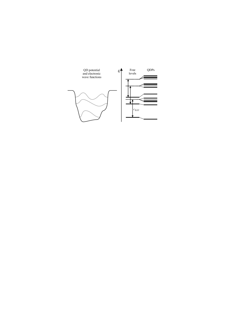
Figure 2: Qualitative structure of the polaron spectrum in the case of three bound, non-degenerate electronic levels. Each gray bar indicates 3 additional polaron levels that would result from interactions with two-phonon states.

In conclusion, a complete non-orthogonal polaron basis called the “natural basis” (28) has been introduced. It provides a mean for physical understanding of polaron spectra involving low phonon numbers, and constitutes a simplifying and powerful computational basis (see III.4, IV).

III.2 Accidental Electronic Degeneracies

This section and the next one point out additional simplifications in the case of electronic degeneracies. In particular, if a non-degenerate electronic spectrum (e.g. Fig. 2) becomes partially degenerate, for example by specific dot size adjustment, not only certain QDPs may become degenerate, but some of them will analytically align with free levels. We shall call such states “zero-shift polarons” and show that they are nothing but uncoupled states, susceptible to become QDPs as soon as the degeneracies are lifted. Thus the relevant Hilbert space $\mathcal{H}^{\ast}$ can be further reduced, such that spurious zero-shift polarons are automatically eliminated.

In order to label accidental degeneracies, the electron index is now expressed as $\mu\equiv(\tau,i)$, where $\tau=1\ldots n<N$ is an energy index and $i=1,\ldots,g_{\tau}$ a degeneracy index. The eigenspaces of $H^{0}$ inside the one-phonon subspace $\mathcal{H}^{QDP}_{1}$ are indexed by $\gamma=\tau$, and the orthogonal projectors $\mathcal{P}_{\gamma}\equiv\mathcal{P}_{\tau}$ on these eigenspaces write $\mathcal{P}_{\tau}=\sum_{i}^{g_{\tau}}\sum_{\mathbf{q}}\big{|}\tau,i;q\big{>}\big{<}\tau,i;q\big{|}$. Substituting these projectors in (24) allows to write the relevant subspace $\mathcal{H}^{\ast}$ as

$$\begin{split}&\mathcal{H}^{\ast}\equiv\mathcal{H}^{QDP}_{0}\oplus\tilde{\mathcal{H}}^{QDP}_{1}\\ &\text{with}\quad\tilde{\mathcal{H}}^{QDP}_{1}=vect\left\{\mathcal{P}_{\tau}H^{int}\big{|}\mu;0\big{>}\ \forall\,\tau,\mu\right\}\\ \end{split}$$ (30)

Expressing $\mathcal{H}^{QDP}_{0}$, $\mathcal{P}_{\tau}$, and $H^{int}$ in basis vectors $\big{|}\mu;0\big{>}$ and $\big{|}\mu;\mathbf{q}\big{>}$, naturally provides a basis of $\mathcal{H}^{\ast}$,

$$\small\mathcal{B}^{\ast}=\Big{\{}\big{|}\tau,i;0\big{>},\sum_{i^{\prime}=1}^{g_{\tau^{\prime}}}\sum_{\mathbf{q}}M^{\ast}_{\tau\,i,\tau^{\prime}\,i^{\prime};\mathbf{q}}\big{|}\tau^{\prime},i^{\prime};\mathbf{q}\big{>}\ \forall\,\tau,\tau^{\prime},i\Big{\}}$$ (31)

Its dimension is

$$dim(\mathcal{H}^{\ast})=card(\mathcal{B}^{\ast})=N(n+1)$$ (32)

where $N$ is the total number of orthogonal electronic states in the dot and $n<N$ is the number of distinct electronic energies (n=N would be the non-degenerate case.) We note, that even though the number of polarons is smaller in the degenerate case, the number of modes involved remains the same. Only the number of accessible product states $\big{|}\text{electron}\big{>}\otimes\big{|}\text{phonon}\big{>}$ is reduced. This can be seen from (31), which, for a degenerate level $\tau$, yields entangled states similar to $\sum_{i^{\prime}}^{g_{\tau^{\prime}}}B_{(\tau,i)(\tau^{\prime},i^{\prime})}^{\dagger}\big{|}\tau^{\prime},i^{\prime};0\big{>}\ \forall\,\tau,i$.

As in the previous section, the natural basis (31) provides a qualitative prediction of the polaronic spectrum and associates each polaron level with a free level (see example Fig. 3). In particular, we emphasize that the highest free level in the figure only yields 3 orthogonal polaron states and not 6 as one might expect from pulling together the two uppermost free levels in Fig. 2. The particular case of symmetry related degeneracies is now addressed in the next subsection.

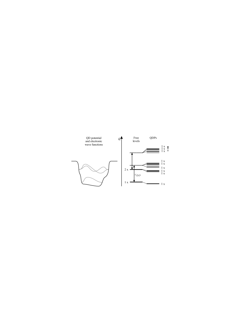
Figure 3: Qualitative structure of the polaron spectrum in the case of two electronic levels, one of which is twice degenerate. Each gray bar indicates 3 more polarons that would result from interactions with two-phonon states.

III.3 Symmetrical Quantum Dots

Additional degeneracies and simplifications may be obtained in the case of QDs invariant under a set of symmetry operations, generally described by the group of such operations $\mathcal{G}$, i. e. $[H,g]=0\ \forall g\in\mathcal{G}$. In such a situation all stationary states satisfy well defined transformation laws, associated with an irreducible representation (irrep) $\Gamma$ of dimension $d_{\Gamma}$, which also specifies the respective level degeneracy. For $d_{\Gamma}>1$, a degeneracy index $j=1,\ldots,d_{\Gamma}$, the so-called “partner function”, labels a choice of orthogonal states within the same eigenspace. Expressed for passive transformations, the laws read

$$\theta(g)^{-1}\psi_{\Gamma,j}=\sum_{i=1}^{d_{\Gamma}}\left(D^{\Gamma}(g)\right)^{-1}_{ij}\psi_{\Gamma,i}\qquad\forall g\in\mathcal{G}\quad$$ (33)

where $D^{\Gamma}(g)$ is a set of representation matrices that characterize the transformation laws of the partner function basis, and can be chosen in a suitable way.

Since all stationary states can be associated with a well defined symmetry $(\Gamma,j)$, the Hamiltonian can be pre-diagonalized by finding an orthogonal decomposition of the Hilbert space in subspaces gathering only states with symmetry $(\Gamma,j)$. As for the one-phonon/one-electron QD model, this symmetry decomposition writes

$$\mathcal{H}^{\ast}=\bigoplus_{\Gamma,j}\mathcal{H}^{\ast}_{\Gamma,j}\ ,\ \ \ \mathcal{H}^{\ast}_{\Gamma,j}\equiv\mathcal{P}_{\Gamma,j}\mathcal{H}^{\ast}$$ (34)

where the orthogonal projectors $\mathcal{P}_{\Gamma,j}$ on the subspaces spanned by all the states that satisfy the transformation laws (33) for a given symmetry $(\Gamma,j)$ can be written as

$$\mathcal{P}_{\Gamma,j}=\frac{d_{\Gamma}}{\left|G\right|}\sum_{g}\Big{(}D^{\Gamma}(g)^{-1}\Big{)}^{\ast}_{jj}\,\,\theta^{-1}(g)$$ (35)

The problem of finding the QDPs reduces to solving $H^{QDP}$ inside each relevant subspace $\mathcal{H}^{\ast}_{\Gamma,j}$ individually. To provide these subspaces with suitable bases, we require a symmetrized eigenstate basis relative to $H^{0}$, i.e. each basis state satisfies the transformation (33) for its particular symmetry $(\Gamma,j)$. Such bases necessarily exist, since $H^{0}$ obeys the same symmetry as $H$. To start with we symmetrize the electron subsystem and the phonon subsystem separately, i.e.

$$\begin{split}electron:\ \ \left\{\big{|}\tau,i\big{>}\right\}\ &\longleftrightarrow\left\{\big{|}\Gamma_{e},j_{e},\alpha_{e}\big{>}\right\}\\ phonon:\ \left\{\big{|}0\big{>},\big{|}\mathbf{q}\big{>}\right\}&\longleftrightarrow\left\{\big{|}0\big{>},\big{|}\Gamma_{ph},j_{ph},\alpha_{ph}\big{>}\right\}\quad\\ \end{split}$$ (36)

$\alpha_{e}$ is usually a sequential index with energy, whereas $\alpha_{ph}$ represents a continuous degeneracy index because of the assumption of LO-phonon monochromaticity. The explicit transformations (36) can be more subtle than anticipated. An example will be developed in detail for the $C_{3v}$ symmetry group in section IV.1. These symmetrized bases allow the construction of a symmetrized basis of the tensorial products using generalized Clebsch-Gordan coefficients $C^{\Gamma,\Gamma_{e},\Gamma_{ph}}_{j,j_{e},j_{ph}}$ (in the sense of point groups),

$$(a) \big{|}\Gamma,j;\Gamma_{e},\alpha_{e};0\big{>}=\big{|}\Gamma_{e}=\Gamma,j_{e}=j,\alpha_{e}\big{>}\otimes\big{|}0\big{>}\qquad$$

$$(b) \big{|}\Gamma,j;\Gamma_{e},\alpha_{e};\Gamma_{ph},\alpha_{ph}\big{>}$$

$$=\sum_{j_{e},j_{ph}}C^{\Gamma,\Gamma_{e},\Gamma_{ph}}_{j,j_{e},j_{ph}}\big{|}\Gamma_{e},j_{e},\alpha_{e}\big{>}\otimes\big{|}\Gamma_{ph},j_{ph},\alpha_{ph}\big{>}$$

Here $\Gamma$ and $j$ refer to the overall symmetry and $\Gamma_{e}$ and $\Gamma_{ph}$ satisfy $\Gamma\subseteq\Gamma_{e}\otimes\Gamma_{ph}$. The phonon vacuum is always symmetrical, $\Gamma_{ph}=A_{1}$, and hence the overall representation of a state with zero phonons will always be identified with the electron representation, $\Gamma=\Gamma_{e}$ (eq. III.3).

A symmetrized expression of the relevant subspace $\mathcal{H}^{\ast}$ immediately results from equation (30) by replacing the electronic energy index $\tau$ with the pair index $(\Gamma_{e},\alpha_{e})$. Expressing $\mathcal{H}^{QDP}_{0}$ and $\mathcal{P}_{\Gamma_{e},\alpha_{e},1\,ph}$ in terms of the symmetrized product basis (III.3) directly leads us to a set of non-orthogonal basis vectors, each of which transforms according to (33) for a particular symmetry $(\Gamma,j)$. Those vectors can be regrouped in different “natural bases” $\mathcal{B}^{\ast}_{\Gamma,j}$ associated with the different subspaces $\mathcal{H}^{\ast}_{\Gamma,j}$ defined in (34). The expression of those vectors can be further simplified using the selection rule for the Fröhlich matrix elements, which results directly from the transformation laws and the invariance of the Hamiltonian,

$$\begin{array}[]{l}\big{<}\Gamma,j;\Gamma_{e},\alpha_{e};\Gamma_{ph},\alpha_{ph}\big{|}H^{int}\big{|}\Gamma^{\prime},j^{\prime};\Gamma_{e}^{\prime}=\Gamma,\alpha_{e};0\big{>}=0\\ \text{unless}\quad(\Gamma,j)=(\Gamma^{\prime},j^{\prime})\end{array}$$

For the remaining non-vanishing matrix elements, we shall use the notation

$$M^{\Gamma,j}_{(\Gamma_{e},\alpha_{e},\Gamma_{ph},\alpha_{ph});\alpha_{e}^{\prime}}\equiv$$ (38)

$$\big{<}\Gamma,j;\Gamma_{e},\alpha_{e};\Gamma_{ph},\alpha_{ph}\big{|}H^{int}\big{|}\Gamma,j;\Gamma,\alpha_{e}^{\prime};0\big{>}$$

Finally, the natural bases $\mathcal{B}^{\ast}_{\Gamma,j}$ write

$$\mathcal{B}^{\ast}_{\Gamma,j}=\left\{\begin{array}[]{l}\big{|}\Gamma,j;\Gamma,\alpha_{e};0\big{>},\\ \sum_{\Gamma_{ph},\alpha_{ph}}M^{\Gamma,j}_{(\Gamma_{e}^{\prime},\alpha_{e}^{\prime},\Gamma_{ph},\alpha_{ph});\alpha_{e}}\\ \times\ \big{|}\Gamma,j;\Gamma_{e}^{\prime},\alpha_{e}^{\prime};\Gamma_{ph},\alpha_{ph}\big{>}\\ \forall\ \alpha_{e},\Gamma_{e}^{\prime},\alpha_{e}^{\prime}\end{array}\right\}$$ (39)

The sum goes over all indices, but one assumes that the Clebsch-Gordan coefficients $C$ vanish, when $\Gamma_{ph}$ does not satisfy a selection rule $\Gamma\subseteq\Gamma_{e}\otimes\Gamma_{ph}$. These bases are mutually orthogonal, but the vectors in each individual basis remain non-orthogonal.

The overall symmetry index of an arbitrary natural basis state is always equal to the symmetry index of the involved pure electron state (zero-phonon state), see equations (38,39). Hence, if an existing representation $\Gamma$ is absent in the considered set of bound electrons, there are no $\Gamma$-like polaron states, even though we necessarily have $\Gamma$-like phonon states!

Like in the previous two sections the natural bases (39) provide a prediction of the polaronic spectrum. Fig. 4 shows the particular case of two bound electronic levels, where the second level is twice degenerate by virtue of the underlying dot symmetry. In particular, we emphasize the appearance of degenerate polaron levels, which can be associated with both, a degenerate or non-degenerate electron level.

The dimensionality of the different subspaces $\mathcal{H}^{\ast}_{\Gamma,j}$ can be derived from the number of natural basis states for a given symmetry $(\Gamma,j)$,

$$dim(\mathcal{H}^{\ast}_{\Gamma,j})=card(\mathcal{B}^{\ast}_{\Gamma,j})=n^{\Gamma}(1+n)$$ (40)

$n^{\Gamma}$ is the number of distinct electronic energies with a given symmetry $\Gamma$ ($\alpha_{e}=1,\dots,n^{\Gamma}$), and $n$ denotes the total number of distinct electronic energies ($n=\sum_{\Gamma}n^{\Gamma}$). The dimension (40) is independent of the partner function $j$ in agreement with the feature that those functions can be defined arbitrarily inside a given representation $\Gamma$. Since $\sum_{(\Gamma,j)}dim(\mathcal{H}^{\ast}_{\Gamma,j})$ equals $dim(\mathcal{H}^{\ast})$, given in (32), expression (40) is a consistent refinement of the full dimension.

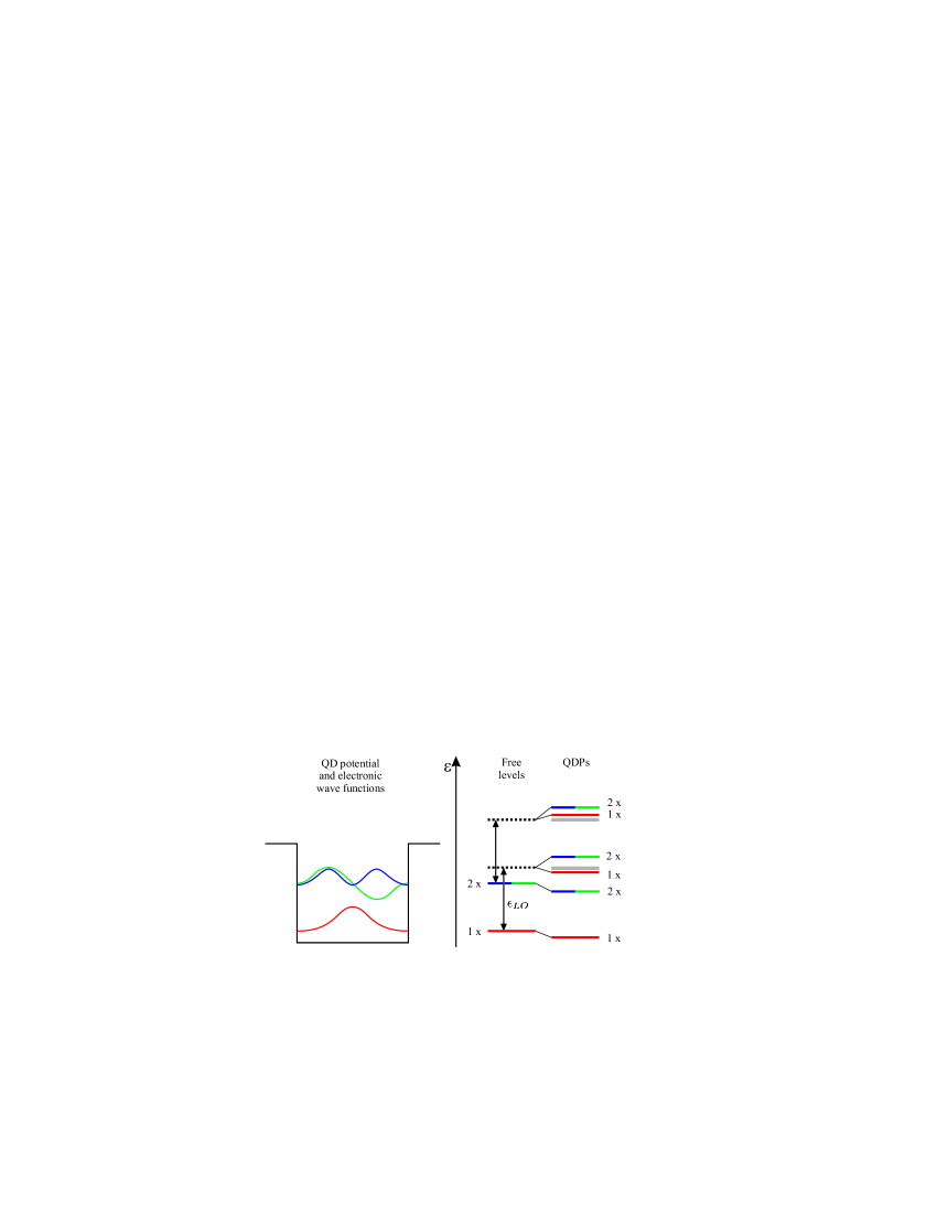
Figure 4: (Color online) Qualitative structure of the polaron spectrum in the case of two electronic levels, one of which is twice degenerate due to the dot symmetry. The levels correspond to two different representations $\Gamma$ marked in red and blue/green. The latter has two dimensions, characterized by the function $j$. Each gray bar indicates 3 more polarons that would result from interactions with two-phonon states.

III.4 Computational Aspects

Finding the polaron spectrum of the one-electron/one-phonon model reduces to diagonalizing the Hamiltonian $H^{QDP}$ inside the low dimensional subspace spanned by the natural basis $\mathcal{B}^{\ast}$ given in (28), (31) or (39), depending on the physical situation. Although the number of Fröhlich matrix elements for the interaction with LO-phonons has been minimized by the subspace reduction, their prerequisite computation can be numerically intensive for the arbitrary 3D wavefunctions that one should consider in a general case (see section IV where a single wavefunction is typically sampled on $10^{6}$ points). To alleviate this issue we have developed an original adaptive, irregular discretization of the reciprocal space for lattice modes, and shown that it was an efficient method, also applicable when working directly with a non-orthogonal basis.

The numerical benefit of an irregular reciprocal space discretization relies on the fast variation of the Fröhlich matrix elements in function of the normal mode wave vector $\mathbf{q}$ in certain well localized domains. Increasing the local point density only in those domains remarkably improves the numerical precision with a minor increase of the required computational resources. To generate a well adapted irregular $\mathbf{q}$-space discretization, we start with a regular coarse mesh covering the first Brillouin zone of the underlying lattice. Then the various Fröhlich matrix elements are evaluated for all wave vectors $\mathbf{q}$ of the given mesh. This requires a preliminary computation of the volumes associated with each mesh node, taken as the volume of the respective Wigner-Seitz cells (Appendix VII.3). The nearest neighbors with the highest difference between their Fröhlich elements are added a new node in between, which provides the initial mesh for the next iteration. This algorithm is repeated until the maximal difference between neighboring Fröhlich matrix elements falls below a preset threshold. Fig. 5 shows the Wigner-Seitz cells generated with this technique in the case of the first Brillouin zone of a body-centered cubic lattice.

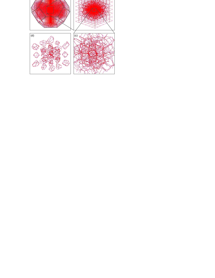
Figure 5: (Color online) Polygonal Wigner-Seitz cells of the irregular $\mathbf{q}$-space discretization. (a)-(c) zoom into first Brillouin zone of a BCC lattice. (d) A few selected Wigner-Seitz cells from a region similar to (c).

After the generation of the irregular $\mathbf{q}$-space discretization and the computation of the respective Fröhlich matrix elements, the set of natural basis vectors is evaluated, allowing to diagonalize the relevant Hamiltonian $H^{QDP}$.

Let us finally evaluate the numerical value of working with a non-orthogonal basis. The sole consequence is that the standard eigenvalue problem becomes a generalized eigenvalue problem, that is an equation of the type

$$\bar{\bar{H}}^{QDP}\big{|}\psi\big{>}=\epsilon\bar{\bar{S}}\big{|}\psi\big{>},$$ (41)

$$\bar{\bar{H}}^{QDP}_{\alpha\alpha^{\prime}}\equiv\big{<}\alpha\big{|}H^{QDP}\big{|}\alpha^{\prime}\big{>},\quad\bar{\bar{S}}_{\alpha\alpha^{\prime}}\equiv\big{<}\alpha|\alpha^{\prime}\big{>}\neq\delta_{\alpha,\alpha^{\prime}}\qquad$$

where $\big{|}\alpha\big{>}$ are the natural basis states, and $\bar{\bar{S}}_{\alpha\alpha^{\prime}}$ is the so-called ”mass matrix”. This trade-off is advantageous, since optimized packages for the generalized eigenvalue problem are widely available, and one gets rid of an additional basis change involving a Gram-Schmidt decomposition (often requiring enhanced precision for small scalar products). This is a positive numerical byproduct of the non-orthogonal theory.

With the set of tools presented above, a spectral precision down to 0.01meV for typical QDPs can be reached in characteristic computation times of a few minutes using a present-day standard processor (3 GHz, 32 bit). The most computer intensive part is the preliminary evaluation of the Fröhlich matrix elements.

IV Application to Pyramidal QDs

IV.1 Symmetrical Model and Non-Orthogonal Basis

In this section, we apply the minimal model for the non-orthogonal theory (section III) to a realistic pyramidal GaAs/AlGaAs QD.Kapon 04 This dot is part of a complex heterostructure represented by the geometrical model shown in Fig. 6a.Michelini 05 We will take full advantage of the underlying $C_{3v}$-symmetry group, which exhibits only three irreps $A_{1}$, $A_{2}$ and $E$. The latter is two-dimensional and a possible basis results from symmetrizing $E$-states with respect to the symmetry plane $\sigma_{1}$ (spanned by the [111] and [112] crystalline directions in GaAs/AlGaAs). Thereby the partner function $j=\pm$ is identified with the parity index relative to $\sigma_{1}$. In graphical representations we shall consistently apply the color scheme: $A_{1}$ (red), $A_{2}$ (yellow), $E+$ (blue), $E-$ (green). QDPs will be computed using the symmetrized natural basis introduced in section III.3. This basis will be derived analytically in three stages: (1) individual symmetrization of electronic and phononic eigenstates of $H^{0}$, (2) construction of a symmetrized product basis using Clebsch-Gordan coefficients, and (3) derivation of the symmetrized natural bases for the relevant subspaces $\mathcal{H}^{\ast}_{\Gamma,j}$.

First, we shall find symmetrized electron and phonon bases. As for the bound electron, all eigenstates of $H^{0}$ are automatically symmetrized and hence the task reduces to finding these eigenstates. This was recently achieved by Michelini et al..Michelini 05 using an effective mass model. For a dot height $h=10nm$, there are two $A_{1}$-like levels (non-degenerate) and one $E$-like level (twice degenerate) as shown in Fig. 6b. In the standard notation of section III.3, i. e. $\big{|}\Gamma_{e}\ j_{e},\alpha_{e}\big{>}$, those states write

$$\Big{\{}\big{|}A_{1},1\big{>},\big{|}E\pm\big{>},\big{|}A_{1},2\big{>}\Big{\}}\ \ electron\ basis$$ (42)

where the index $j_{e}$ has been omitted in the case of the one-dimensional $A_{1}$-representations and the index $\alpha_{e}$ has been omitted for the unique $E$-level. We note that there are no $A_{2}$-like electron states at low energy, which immediately predicts that there will be no $A_{2}$-like QDPs (section III.3). For the phonons (taken as bulk phonons) the symmetrization is inasmuch different as the eigenstates of $H^{0}$, such as plane waves $\xi_{\mathbf{q}}(\mathbf{x})$, are not automatically symmetrized. This feature relies on the monochromaticity assumption rendering all normal modes degenerate. A symmetrized eigenstate basis is properly derived in Appendix VII.4. The resulting basis states superpose six (or four) plane waves, such that the directions of the different wave vectors are mutually related by symmetry operations (see Fig. 6c). We shall label such states with the respective vector $\tilde{\mathbf{q}}$ belonging to the subset $\mathcal{A}$, which constitutes a sixth of the reciprocal space. In the case of $E$-like superpositions there are two orthogonal states associated with the same vector $\tilde{\mathbf{q}}$. They will be distinguished through the additional index $\chi=1,2$ (discussion in Appendix VII.4). Finally the phonon basis writes

$$\left\{\begin{array}[]{l}\big{|}0\big{>},\big{|}A_{1},\tilde{\mathbf{q}}\big{>},\big{|}A_{2},\tilde{\mathbf{q}}\big{>},\\ \big{|}E\pm,\tilde{\mathbf{q}},\chi\big{>}\end{array}\right\}\ \ phonon\ basis$$ (43)

where $\big{|}0\big{>}$ is the phonon vacuum state (0meV), whilst all other states are one-phonon states (35.9meV).

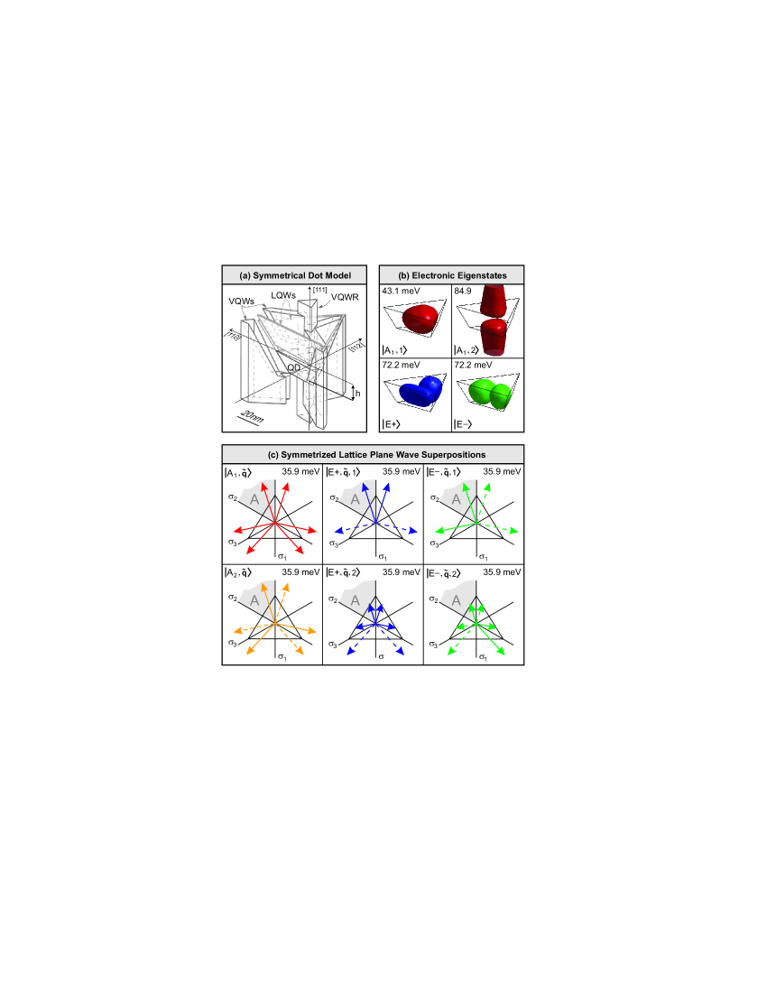
Figure 6: (Color) (a) Numerical model Michelini 05 of realistic heterostructure with pyramidal QD, vertical quantum wire (VQWR), vertical quantum wells (VQWs) and lateral quantum wells (LQWs). (b) Isosurfaces of envelope functions of the stationary single electron states. (c) Particular plane wave superpositions of symmetrized one-phonon basis. The length of the arrows represents the relative amplitude and dashed arrows have opposite phase.

Second, we construct a symmetrized product basis from (42) and (43) according to Eq.(III.3). The explicit derivations given in Appendix VII.5 yield states of the form

$$\left\{\begin{array}[]{l}\big{|}\Gamma\ j;\Gamma_{e},\alpha_{e};0\big{>},\\ \big{|}\Gamma\ j;\Gamma_{e},\alpha_{e};\Gamma_{ph},\tilde{\mathbf{q}},\chi\big{>}\end{array}\right\}\ \ product\ basis$$ (44)

where the first ket represents states with zero phonons and the latter states with one phonon.

Third, we write the natural basis of the relevant Hilbert subspace of $\mathcal{H}^{\ast}$ according to the general theory (section III.3). This basis decomposes in symmetry-subspaces $\mathcal{H}^{\ast}_{A_{1}}$ (8 dimensions), $\mathcal{H}^{\ast}_{E+}$ (4 dimensions), $\mathcal{H}^{\ast}_{E-}$ (4 dimensions). Yet, in our particular case the most energetic natural basis states yield energies above the first two-phonon state. To remain consistent with the one-phonon assumption, we shall neglect those states. Thereby the dimensions reduce to 6 ($\mathcal{H}^{\ast}_{A_{1}}$), 3 ($\mathcal{H}^{\ast}_{E+}$) and 3 ($\mathcal{H}^{\ast}_{E-}$). The respective natural bases result from the general expressions (39) and are given in Tab. 1 and Tab. 2.

meV	expressed as symmetrized product states	subspace
43.1	$\big{|}A_{1};A_{1},1;0\big{>}$	$\mathcal{H}^{\ast}_{A_{1},1}$
79.0	$\sum_{\tilde{\mathbf{q}}}\big{|}A_{1};A_{1},1;A_{1},\tilde{\mathbf{q}}\big{>}\big{<}...\big{|}H^{int}\big{|}A_{1};A_{1},1;0\big{>}$
108.1	$\sum_{\tilde{\mathbf{q}},\chi}\big{|}A_{1};E;E,\tilde{\mathbf{q}},\chi\big{>}\big{<}...\big{|}H^{int}\big{|}A_{1};A_{1},1;0\big{>}$
84.9	$\big{|}A_{1};A_{1},2;0\big{>}$	$\mathcal{H}^{\ast}_{A_{1},2}$
79.0	$\sum_{\tilde{\mathbf{q}}}\big{|}A_{1};A_{1},1;A_{1},\tilde{\mathbf{q}}\big{>}\big{<}...\big{|}H^{int}\big{|}A_{1};A_{1},2;0\big{>}$
108.1	$\sum_{\tilde{\mathbf{q}},\chi}\big{|}A_{1};E;E,\tilde{\mathbf{q}},\chi\big{>}\big{<}...\big{|}H^{int}\big{|}A_{1};A_{1},2;0\big{>}$

Table 1: Natural basis states of the subspace $\mathcal{H}^{\ast}_{A_{1}}$. The bra $\big{<}...\big{|}$ is the adjoint of the preceding ket. The two subspaces $\mathcal{H}^{\ast}_{A_{1},1}$ and $\mathcal{H}^{\ast}_{A_{1},2}$ are defined by the three basis vectors on their left. They constitute so-called “weakly coupled strong coupling regimes”, discussed in section IV.3.

meV	expressed as symmetrized product states
72.2	$\big{|}E\pm;E;0\big{>}$
79.0	$\sum_{\tilde{\mathbf{q}},\lambda}\big{|}E\pm;A_{1},1;E,\tilde{\mathbf{q}},\lambda\big{>}\big{<}...\big{|}H^{int}\big{|}E\pm;E;0\big{>}$
108.1	$\sum_{\Gamma_{ph},\tilde{\mathbf{q}},\chi}\big{|}E\pm;E;\Gamma_{ph},\tilde{\mathbf{q}},\chi\big{>}\big{<}...\big{|}H^{int}\big{|}E\pm;E;0\big{>}$

Table 2: Natural basis states of subspaces $\mathcal{H}^{\ast}_{E+}$ and $\mathcal{H}^{\ast}_{E-}$. The bra $\big{<}...\big{|}$ is the adjoint of the preceding ket.

IV.2 Stationary States and Strong Coupling

The problem of finding the stationary dot states, i.e. QDPs, consists in the eigenvalue problem

$$H^{QDP}\big{|}\Gamma\,j,m\big{>}=\epsilon_{\Gamma,m}\big{|}\Gamma\,j,m\big{>}$$ (45)

where $m$ is a sequential energy index inside a particular symmetry $(\Gamma,j)$. This eigenvalue equation was solved individually inside each of the three decoupled subspaces $\mathcal{H}^{\ast}_{A_{1}}$, $\mathcal{H}^{\ast}_{E+}$ and $\mathcal{H}^{\ast}_{E-}$ using the enhanced matrix diagonalization method outlined in section III.4. The three resulting spectra are given in Fig. 7 (red, green, blue). A geometrical representation of the corresponding polaron states is shown in Fig. 8, where the closed surfaces are isosurfaces of the electronic and vibrational probability density functions. Those functions were obtained by computing the respective partial traces,

$$\rho_{lattice}(\mathbf{x}) = \big{<}\mathbf{x}\big{|}Tr_{electron}\Big{(}\big{|}\Gamma\,j,m\big{>}\big{<}\Gamma\,j,m\big{|}\Big{)}\big{|}\mathbf{x}\big{>}\qquad$$ (46)

$$\rho_{electron}(\mathbf{x}) = \big{<}\mathbf{x}\big{|}Tr_{lattice}\Big{(}\big{|}\Gamma\,j,m\big{>}\big{<}\Gamma\,j,m\big{|}\Big{)}\big{|}\mathbf{x}\big{>}$$ (47)

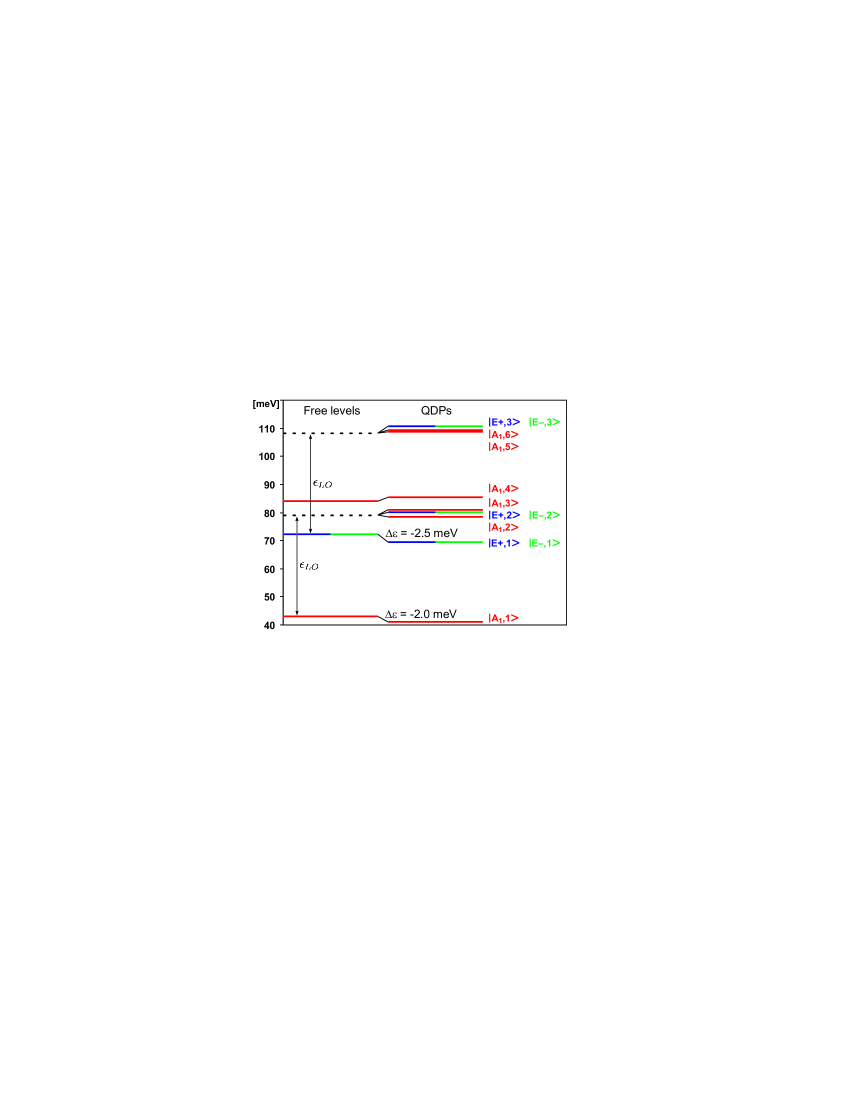
Figure 7: (Color) Spectrum of low energy quantum dot polarons (QDPs). Inside each symmetry subspace the states have been labeled with an energy index $m$, such that $m=1$ corresponds to lowest energy state of a given symmetry.

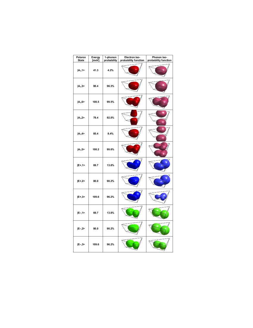
Figure 8: (Color) Geometrical representation of QDPs. The two right columns show isosurfaces of the electronic and vibrational probability density functions in direct space.

The two-dimensional representation $E$ necessarily exhibits a spectrum consisting of twice degenerate levels, each of which is associated with one state in $\mathcal{H}^{\ast}_{E+}$ and one state in $\mathcal{H}^{\ast}_{E-}$. Each superposition $c_{+}\big{|}E+,m\big{>}+c_{-}\big{|}E-,m\big{>}$ is again a stationary state.

Both the ground level and the first excited level yield negative energy shifts. This is consistent with the general feature that the ground level of each representation is necessarily lowered with respect to corresponding free level. The numerical values of these shifts are $\Delta\varepsilon=-2.0\ meV$ and $\Delta\varepsilon=-2.5\ meV$. The same shifts computed with 2nd order perturbation theory are $\Delta\varepsilon=-7.0\ meV$ and $\Delta\varepsilon=-17.4\ meV$, respectively. This manifest large failure of a perturbative approach clearly confirms the existence of a strong coupling inside both irreps ($A_{1}$, $E$).

IV.3 Coupling Substructure

For further characterization of the coupling regime it is interesting to consider the two state sets $\mathcal{S}_{1}$ and $\mathcal{S}_{2}$, defined as

$$\begin{split}\mathcal{S}_{1}&\equiv\left\{\big{|}A_{1},1\big{>},\big{|}A_{1},3\big{>},\big{|}A_{1},6\big{>}\right\}\\ \mathcal{S}_{2}&\equiv\left\{\big{|}A_{1},2\big{>},\big{|}A_{1},4\big{>},\big{|}A_{1},5\big{>}\right\}\\ \end{split}$$ (48)

The $A_{1}$-states of Fig. 8 have been ordered according to these sets. We demonstrated numerically that states in $\mathcal{S}_{1}$ are to a good approximation contained in the subspace $\mathcal{H}^{\ast}_{A_{1},1}\subset\mathcal{H}^{\ast}_{A_{1}}$ defined in Tab. 1. Indeed, the norms of their projections on $\mathcal{H}^{\ast}_{A_{1},1}$ exceed 95% of the full norms. With the same accuracy the states in $\mathcal{S}_{2}$ are contained in $\mathcal{H}^{\ast}_{A_{1},2}\subset\mathcal{H}^{\ast}_{A_{1}}$. In other words, the two subspaces $\mathcal{H}^{\ast}_{A_{1},1}$ and $\mathcal{H}^{\ast}_{A_{1},2}$ appear reasonably decoupled, although the whole subspace $\mathcal{H}^{\ast}_{A_{1}}\equiv\mathcal{H}^{\ast}_{A_{1},1}\oplus\mathcal{H}^{\ast}_{A_{1},2}$ constitutes a strong coupling regime. Therefore the strong coupling regime must reside inside the two subspaces $\mathcal{H}^{\ast}_{A_{1},1}$ and $\mathcal{H}^{\ast}_{A_{1},2}$ individually, and they may be referred to as “weakly coupled strong coupling regimes”. The physical reason for this particular structure relies in the geometry of the vibrational density function $\rho_{lattice}(\mathbf{x})$. Fig. 8 shows that states in $\mathcal{S}_{1}$ have a vibrational component, which is vertically centered in the dot, whereas the states in $\mathcal{S}_{2}$ have two centers of vibration splitting the isosurface in two parts. Indeed the subspace $\mathcal{H}^{\ast}_{A_{1},1}$ is spanned by two one-phonon states with vertically centered vibrational density and one zero-phonon state with centered electronic density. The resulting overlap leads to a strong interaction between electrons and phonons. The same conclusion applies to the subspace $\mathcal{H}^{\ast}_{A_{1},2}$, where the density functions are vertically split in two parts. One the other hand, this picture reveals that the mutual overlap between $\mathcal{H}^{\ast}_{A_{1},1}$ and $\mathcal{H}^{\ast}_{A_{1},2}$ is considerably smaller.

The concept of weakly coupled subspaces $\mathcal{H}^{\ast}_{A_{1},1}$ and $\mathcal{H}^{\ast}_{A_{1},2}$ provides a direct tool for interpretation of the spectrum in Fig. 7. In particular, the ground levels of each subspace, i.e. $\big{|}A_{1},1\big{>}$ and $\big{|}A_{1},2\big{>}$, are necessarily lowered relative to the corresponding free levels. Analogically, the most excited levels of each subspaces, i.e. $\big{|}A_{1},5\big{>}$ and $\big{|}A_{1},6\big{>}$, are both raised. Their mutual splitting remains very small as they are to a good approximation uncoupled.

Finally, we emphasize that the novel concept of “weakly coupled strong coupling regimes”, represented by the subspaces $\mathcal{H}^{\ast}_{\Gamma\,j,1}$ and $\mathcal{H}^{\ast}_{\Gamma\,j,2}$,$\ldots$, is very general and potentially applicable to all QDs. If the matrix element integral is close to zero due to the mutual orthogonality of the electronic wave functions, these subspaces can be treated as decoupled in a good approximation. This idea is straightforward when working with the natural basis, and thus represents a further advantage of using non-orthogonal basis states.

IV.4 Entanglement measure and strong coupling, decoherence and relaxation

An alternative characterization of the strong coupling is reflected in the entanglement of stationary dot states, i.e. QDPs. We have computed the entanglement between electronic and and phononic coordinates using the standard measure introduced by Bennett et al..Bennett 96 For pure states,

$$Ent\big{(}\big{|}\Gamma\,j,m\big{>}\big{)}\equiv-\sum_{i=1}^{N}{\left|c_{i}\right|^{2}log_{N}\left|c_{i}\right|^{2}}$$ (49)

where the coefficients $c_{i}$ are given by the diagonal Schmidt decomposition

$$\big{|}\Gamma\,j,m\big{>}=\sum_{i=1}^{N}c_{i}\big{|}e_{i}\big{>}\otimes\big{|}ph_{i}\big{>}$$ (50)

It is known that this form always exists for every particular ket $\big{|}\Gamma\,j,m\big{>}$, but the computation of the $\big{|}\Gamma\,j,m\big{>}$-dependent orthogonal vectors $\left\{\big{|}e_{i}\big{>}\right\}$ and $\left\{\big{|}ph_{i}\big{>}\right\}$, in the electronic and phononic Hilbert spaces respectively, now requires a preliminary orthogonalization of the quantum dot phonon basis $B^{\dagger}_{\mu\mu^{\prime}}\big{|}0\big{>}$ which can be elegantly performed via a Choleski decomposition of the $\Lambda$ matrix. A subsequent singular value decomposition (SVD) of the coefficient matrix in the tensorial product basis will deliver $c_{i}$. It is remarkable that the sum over $i$ in (50) can be limited to the number of electron states $N$ because of the properties of the SVD. The entanglement measure (49) can vary between 0 (non-entangled) and 1 (fully entangled), and is also often equivalently called the ”entropy of mixing” of the two subsystems in state $\big{|}\Gamma\,j,m\big{>}$.

Tab. 3 shows the entanglement of the QDPs presented in Fig. 8. Weakly entangled states ($Ent\lesssim 0.1$) are nearly simple product states of electrons and phonons. In the present case, such a picture applies to the two QDPs $\big{|}A_{1},1\big{>}$ and $\big{|}A_{1},3\big{>}$. Numerically, they consist to 99.5% of two natural basis states, which both involve the same electronic state $\big{|}A_{1},1\big{>}$ (first two basis states in Tab. 1). All other QDPs are strongly entangled ($Ent\gtrsim 0.1$) with no adequate perturbative picture. Particularly strong entanglement is found in the states $\big{|}A_{1},5\big{>}$ and $\big{|}A_{1},6\big{>}$, which involve peculiar Bell-state superpositions inside the $E$-representation of the form $\big{|}E+\big{>}\otimes\big{|}E+\big{>}+\big{|}E-\big{>}\otimes\big{|}E-\big{>}$. This of course suggests a general tendency to find particularly strongly entangled polarons in dots with symmetry related degeneracies.

State	Entanglement	Phonon Number	Relax. Factor
$\big{|}A_{1},1\big{>}$	0.023	0.042	0.001
$\big{|}A_{1},3\big{>}$	0.007	0.963	0.007
$\big{|}A_{1},6\big{>}$	0.523	0.995	0.520
$\big{|}A_{1},2\big{>}$	0.203	0.920	0.186
$\big{|}A_{1},4\big{>}$	0.222	0.084	0.019
$\big{|}A_{1},5\big{>}$	0.517	0.996	0.515
$\big{|}E\pm,1\big{>}$	0.256	0.136	0.035
$\big{|}E\pm,2\big{>}$	0.245	0.902	0.221
$\big{|}E\pm,3\big{>}$	0.229	0.962	0.220

Table 3: Entanglement, 1-phonon probability and heuristic “relaxativity measure” of the Quantum Dot Polarons (QDPs) in the pyramidal dot with $h=10mn$.

Finally, we address a possible connection between entanglement and phonon-mediated decoherence and relaxation. A simple model of such decoherence and relaxation would account for a weak bulk interaction between coupled LO-phonons and uncoupled LO-phonons or between coupled LO-phonons and LA-phonons. Such weak interactions maybe treated perturbatively and typically result in a finite lifetime for QDPs, which would otherwise be everlasting. One may expect that the lifetime depends on the entanglement between electronic and phononic coordinates, since entanglement indicates strong quantum correlations that could effectively translate phonon-phonon interactions to electron state hoppings. From this picture, we expect that the lifetime also scales with the weight of the phonon component. Hence, we heuristically propose a “relaxativity measure” for QDPs, defined as the product of the entanglement and the average phonon number

$$Rel\big{(}\big{|}\Gamma\,j,m\big{>}\big{)} \equiv \big{<}\Gamma\,j,m\big{|}\sum_{\lambda\lambda^{\prime}}(\Lambda^{-1})_{\lambda^{\prime}\lambda}B_{\lambda}^{\dagger}B_{\lambda^{\prime}}\big{|}\Gamma\,j,m\big{>}$$ (51)

$$\;\times Ent\big{(}\big{|}\Gamma\,j,m\big{>}\big{)}$$

In the present one-phonon model this measure varies between 0 (everlasting) and 1 (short coherence time, say $\sim 1ps$). At thermal equilibrium, the dot state is represented by a density matrix exhibiting a high probability of states with a low relaxativity measure and vise versa. This measure does not really measure the relaxation since relaxation also implies other factors like resonances and population of final states, this is why we speak of ”relaxativity”. It has the status of a rough heuristic guess, since it is not the result of a proper relaxation model describing realistically phonon-phonon interactions and in particular neglects any dependence on the particular geometry.

IV.5 Dot size variation

We shall now discuss the variation of the polaron spectrum as a function of a varying dot height $h$. Figure 9 shows the varying spectrum of $H^{0}$ (free levels) and the spectrum of $H^{QDP}$ (quantum dot polarons) in the restricted energy band $[40\ meV,\ 120\ meV]$ (quadratically extrapolated from explicit computations of the dot heights 10 nm, 7.5 nm and 5 nm). To gain clarity and to remain consistent with the disappearance of certain free levels for smaller dots, we have restricted the graph to the two lowest levels of the two subspaces $\mathcal{H}^{\ast}_{A_{1},1}$ and $\mathcal{H}^{\ast}_{E+}$. The latter is of course degenerate with $\mathcal{H}^{\ast}_{E-}$ and the respective levels are twice degenerate.

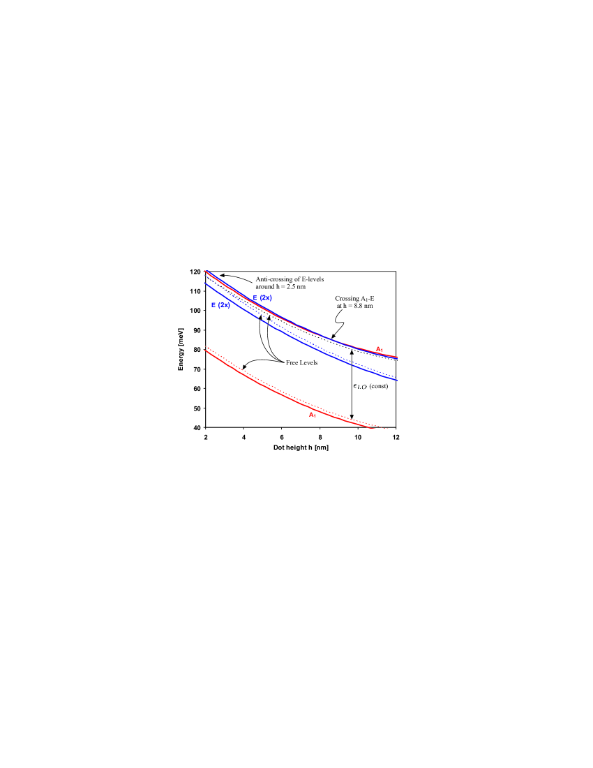
Figure 9: (Color online) Spectrum in function of the dot height $h$. (dashed lines) free electronic energies obtained by diagonalizing $H^{0}$, (solid lines) polaron energies obtained by diagonalizing $H^{QDP}$.

There are three relevant free energies, the electronic ground level with symmetry $A_{1}$ (red dashed line), the first excited level with symmetry $E$ (blue dashed line), and the electronic ground level combined with one phonon (black dashed line). The latter two undergo a crossing in the vicinity of the dot height $h=2.5nm$. By virtue of the resulting resonance, the two $E$-like polaron levels (blue solid lines) exhibit maximal energy shifts around $h=2.5nm$ ($\Delta\epsilon\approx 5\ meV$) giving rise to a level anti-crossing. On the other hand, the decreasing resonance for increasing dot height, leads to a true crossing between the first excited $E$-like polaron level (upper blue solid line) and the first excited $A_{1}$-like polaron level (upper red solid line). Such a true crossing is consistent with the strict analytical decoupling stemming from group theoretical arguments (i.e. different irreps).

V Insights on the low energy scheme in QDs

We shall now expand the results to a very general class of QDs, including pyramidal, spherical, cubic or even cylindrical ones. For all these systems we uncover an analogous low energy spectrum, clear connections between polarons and free levels, symmetry properties and qualitative dot size dependencies.

Explicitly, we consider all dots with a non-degenerate electronic ground level and a twice degenerate first electronic excitation. These dots include the special but predominant class of dots with $C_{nv}$ symmetry with $n\geq 3$. Qualitatively, they yield a low-energy polaron spectrum consisting of two shifted electron levels and a splitted electron+phonon level, see Fig. 10. Group theory reveals three independent substructures (red, green, blue), where two are mutually degenerate (green/blue). This structure can be derived from the natural basis (39), or may be obtained from the spectrum studied above (Fig. 7) by suppressing all QDPs with higher energies or associated with the third electron level.

The fine dashed lines in Fig. 10 link each QDP level with the free level, from which it would arise, if one could continuously turn on the Fröhlich interaction. These connections are important for understanding the QDP spectrum, as levels within the same representation (here the levels with the same color) generally repel each other under the interaction. The relative position of the first excited polaron in the invariant representation (here $\big{|}A_{1},3\big{>}$) depends on whether the free electronic energy spacing is larger or smaller than the constant phonon energy $\epsilon_{LO}$, see Fig. 10a and Fig. 10b. In case (a), the state $\big{|}A_{1},3\big{>}$ can fall between the second electron level (green/blue) and the electron+phonon level (dashed level). In (b), the same state lies always above the free electron+phonon level. One can generally pass from situation (a) to (b) by a dot size increase rendering the electronic energy spacing smaller than $\epsilon_{LO}$.

Further, the links between free levels and QDP levels allow to predict the variation of QDP levels with varying dot size. In general, the shifts become larger as one approaches the resonance, which is the transition between case (a) and (b). The varying spacing between the upper two free levels leads to a changing shift of the two degenerate QDP levels (green/blue). These changes are represented by the vertical arrows for increasing dot size. The dependance gets reversed when passing from case (a) to (b), due to the anti-crossing at the resonance. The shift of the two symmetrical polaron levels (red) is dot size independent, because of their symmetry-decoupling from the moving free level (green/blue) and the constant phonon energy $\epsilon_{LO}$.

These findings are very generic. For example they agree with the results of Verzelen et al. Verzelen 00 for the case of cylindrical dots (height/radius=12/18). Case (a) is obtained for radii $<13$ nm, whilst case (b) correspond to radii $>13$ nm. Following our discussion, it is straightforward to understand that in their case $\big{|}1\pm\big{>}$ lies below $\big{|}S1\big{>}$, that $\big{|}2\pm\big{>}$ lies above $\big{|}P\pm 0\big{>}$ and that $\big{|}\tilde{S}1\big{>}$ can only lie below $\big{|}P\pm 0\big{>}$ for radius $<13$ nm. We also see that the shifts of $\big{|}\tilde{S}0\big{>}$ and $\big{|}\tilde{S}1\big{>}$ do not depend on the dot size due to symmetry decoupling and the constant spacing between $\big{|}S0\big{>}$ and $\big{|}S1\big{>}$.

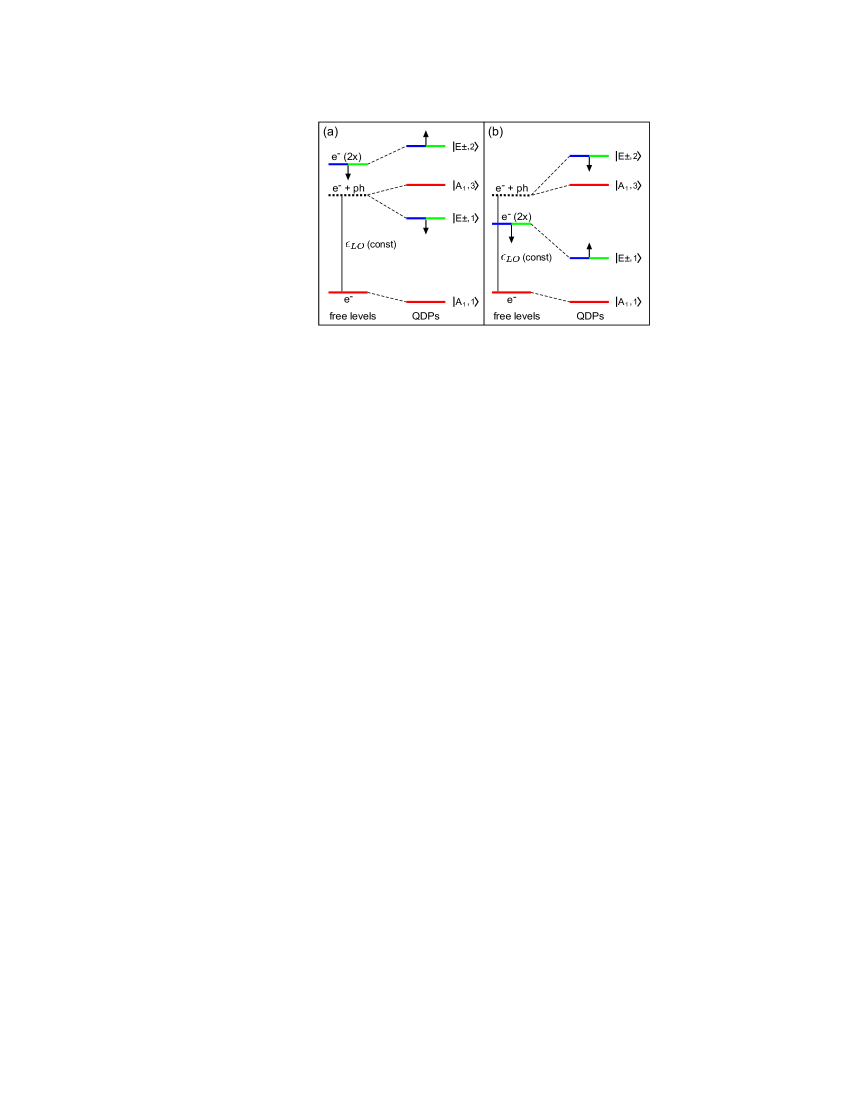
Figure 10: (Color online) Fundamental level structure for QDs with $C_{nv}$-like symmetry with $n\geq 3$. (a) electronic energy spacing exceeds phonon energy $\epsilon_{LO}$, typically smaller dots. (b) electronic energy spacing smaller than $\epsilon_{LO}$, typically larger dots. The arrows show the level changes with increasing dot size.

VI Summary

In this work we uncovered the substantial advantage of the direct use of non-orthogonal creation and annihilation operators to treat polarons in quantum structures. Starting from a general viewpoint, we fully reformulated the polaron problem in terms of those operators that naturally appear in the interaction Hamiltonian and generate the phonons relevant for individual transitions between electronic eigenstates. We also provided a complementary basis for all non-coupling phonons, which play a sensitive role in relaxation processes mediated by phonon-phonon interactions. Even though one might a priori be skeptic with the use of non-orthogonal objects, this approach proved mathematically elegant and fruitful for physical insights. In particular, we found a nested structure in the electron-phonon coupling, which allowed us to identify a non-trivial rule to truncate the Hilbert space in the case of a finite number of phonons. This feature was consistently applied to a general QD structure in a one-electron/one-phonon model, and lead to a novel polaron basis, baptized the “natural basis”. The latter constitutes an efficient tool for computation and detailed classification of quantum dot polarons (QDPs). Beyond the case of general quantum dots, we also investigated degenerate and symmetrical quantum dots using the appropriate mathematical instruments, namely group theory. This revealed additional simplifications, degeneracies and subclasses of QDPs.

As a realistic application we computed the low-energy QDPs of recently manufactured pyramidal QDs with $C_{3v}$-symmetry. To this end an adaptive irregular discretization of the lattice mode space was developed, which we used to compute the Fröhlich matrix elements. The generalized eigenvalue problem stemming from the direct use of non-orthogonal basis vectors was directly fed into efficient matrix diagonalization software. In this way, the requirement for computational resources was remarkably decreased. The numerical results explicitly revealed the spectral structure predicted from the natural basis. 3D-visualizations of the stationary polaronic dot states gave insight in the localization of both electronic and phononic components and showed the different symmetry properties. Dot size dependent spectral investigations uncovered level crossings and anti-crossings, which were consistent with the corresponding symmetry properties. Further, we could prove the existence of strong coupling regimes for each symmetry representation through explicit comparison with second order perturbation theory. Yet, there was undoubtable numerical evidence for the presence of very weakly coupled subspaces within the strong coupling regimes. This led us to the concept of “weakly coupled strong coupling regimes”. Using the natural basis such subspaces could be understood in terms of specifically different overlaps between electronic wave functions and non-orthogonal vibrational modes. We used Bennett’s entanglement measure to quantify the coupling between electronic and phononic coordinates $-$ an idea that finally lead us to a heuristic “relaxativity measure”. In the end, we discussed the low-energy spectrum of an important class of symmetric QDs (including spherical, cubic and cylindrical dots), and showed qualitative predictions of the level structure and dot size dependance, valid as much for the general case as for our specific $C_{3v}$ pyramidal QD.

We thank Paweł Machnikowski and our referees for their thorough and inspiring suggestions. Further, we acknowledge partial financial support from the Swiss NF project No. 200020-109523.

VII Appendix

VII.1 Derivation of the coefficients $c_{\mathbf{q}\mathbf{q}^{\prime}}$

In section II.2, the coefficients $c_{\mathbf{q}\mathbf{q}^{\prime}}$ were defined as

$$B_{\mathbf{q}}^{\dagger}\equiv\sum_{\mathbf{q}^{\prime}}{c_{\mathbf{q}\mathbf{q}^{\prime}}{b_{\mathbf{q}^{\prime}}}^{\dagger}}$$ (52)

such that $B_{\mathbf{q}}^{\dagger}\big{|}0\big{>}=(\openone-\mathcal{P})\,b_{\mathbf{q}}^{\dagger}\big{|}0\big{>}$ with $\mathcal{P}$ being the orthogonal projector onto $vect\{B_{\lambda}^{\dagger}\big{|}0\big{>}\}$. By substitution we find

$$\sum_{\mathbf{q}^{\prime}}{c_{\mathbf{q}\mathbf{q}^{\prime}}{b_{\mathbf{q}^{\prime}}}^{\dagger}}\big{|}0\big{>}=(\openone-\mathcal{P})\,b_{\mathbf{q}}^{\dagger}\big{|}0\big{>}$$ (53)

The projector $\mathcal{P}$ satisfies

$$\mathcal{P}B^{\dagger}_{\lambda}\big{|}0\big{>}=B^{\dagger}_{\lambda}\big{|}0\big{>}$$ (54)

and can be decomposed as

$$\mathcal{P}=\sum_{\lambda\lambda^{\prime}}p_{\lambda\lambda^{\prime}}B^{\dagger}_{\lambda}\big{|}0\big{>}\big{<}0\big{|}B_{\lambda^{\prime}}$$ (55)

with complex coefficients $p_{\lambda\lambda^{\prime}}$. Substituting (55) in (54) and using the commutation relations (6) yields the unique solution $p_{\lambda\lambda^{\prime}}=(\Lambda^{-1})_{\lambda\lambda^{\prime}}$. Hence,

$$\begin{split}\mathcal{P}&=\sum_{\lambda\lambda^{\prime}}(\Lambda^{-1})_{\lambda\lambda^{\prime}}B^{\dagger}_{\lambda}\big{|}0\big{>}\big{<}0\big{|}B_{\lambda^{\prime}}\\ &=\sum_{\mathbf{q}\mathbf{q}^{\prime}}\sum_{\lambda\lambda^{\prime}}(\Lambda^{-1})_{\lambda\lambda^{\prime}}L^{\ast}_{\lambda\mathbf{q}}L_{\lambda^{\prime}\mathbf{q}^{\prime}}b^{\dagger}_{\mathbf{q}}\big{|}0\big{>}\big{<}0\big{|}b_{\mathbf{q}^{\prime}}\\ \end{split}$$ (56)

Substituting (56) into (53) finally exhibits the unique solution

$$c_{\mathbf{q}\mathbf{q}^{\prime}}=\delta_{\mathbf{q}\mathbf{q}^{\prime}}-\sum_{\lambda\lambda^{\prime}}(\Lambda^{-1})_{\lambda\lambda^{\prime}}L^{\ast}_{\lambda\mathbf{q}^{\prime}}L_{\lambda^{\prime}\mathbf{q}}$$ (57)

VII.2 Demonstration of equation (22)

We want to find the $p$-phonon part $\tilde{\mathcal{H}}^{QSP}_{p}$ of a subspace $\mathcal{S}$, defined as

$$\mathcal{S}\equiv vect\Big{\{}e^{-iH^{QSP}t}\big{|}\varphi\big{>}:\forall\,t,\ \forall\,\big{|}\varphi\big{>}\in\mathcal{H}^{QSP}_{p-1}\Big{\}}$$ (58)

In the following, we implicitly assume that $\big{|}\varphi\big{>}$ goes over all states of $\mathcal{H}^{QSP}_{p-1}$ (or, equivalently, over a basis of $\mathcal{H}^{QSP}_{p-1}$). In the expansion of the exponential, the functions $1,t,t^{2},t^{3},\ldots$ are linearly independent. Thus,

$$\mathcal{S}=vect\Big{\{}(H^{QSP})^{k}\big{|}\varphi\big{>}\,\ \forall\ k=0,1,\ldots\Big{\}}$$ (59)

We then replace $H^{QSP}$ by $H^{0}+H^{int}_{+}+H^{int}_{-}$, where $H^{int}_{+}$ is the phonon creating term of $H^{int}$ and $H^{int}_{-}$ is the phonon annihilating term ($H^{int}=H^{int}_{+}+H^{int}_{-}$),

$$\mathcal{S}=vect\Big{\{}(H^{0}+H^{int}_{+}+H^{int}_{-})^{k}\big{|}\varphi\big{>}\,\forall\,k=0,\ldots\Big{\}}\$$ (60)

As we are interested in the $p$-phonon subspace of $S$, the terms $(H^{0}+H^{int}_{+}+H^{int}_{-})^{k}$ can be significantly simplified by retaining only the operator products increasing the phonon number by one unit. These are the products, which contain exactly one more $H^{int}_{+}$ than $H^{int}_{-}$. Further, we want to respect the assumed truncation of the phonon Fock space to at most $p$ phonons, that is imposing $B^{\dagger}_{\lambda}\big{|}\varphi\big{>}=0\ \forall\ \big{|}\varphi\big{>}\in\mathcal{H}^{QSP}_{p}$ (see section II.3). Explicitly, we need to remove all products involving intermediate $(p+1)$-phonon states (e.g. $H^{int}_{-}{H^{int}_{+}}^{2}\big{|}\varphi\big{>}$, which involves the state ${H^{int}_{+}}^{2}\big{|}\varphi\big{>}$). Applying these rules, the terms $(H^{0}+H^{int}_{+}+H^{int}_{-})^{k}\big{|}\varphi\big{>}$ reduce to

$$k=1 : H^{int}_{+}\big{|}\varphi\big{>}$$

$$k=2 : (H^{0}H^{int}_{+}+H^{int}_{+}H^{0})\big{|}\varphi\big{>}$$

$$k=3 : ({H^{0}}^{2}H^{int}_{+}+H^{0}H^{int}_{+}H^{0}+H^{int}_{+}{H^{0}}^{2}$$

$$+{H^{int}_{+}}^{2}H^{int}_{-}+H^{int}_{+}H^{int}_{-}H^{int}_{+})\big{|}\varphi\big{>}$$

$$etc.$$

Since these vectors are used to span a collective subset, we can merely clean the list by creating new superpositions. Explicitly, we walk down the list from $k=1,2,\ldots$ and subtract all the parts that are manifestly covered by smaller $k$ already. For $k=2$, for example, we can subtract $H^{int}_{+}H^{0}\big{|}\varphi\big{>}$ from $(H^{0}H^{int}_{+}+H^{int}_{+}H^{0})\big{|}\varphi\big{>}$, since $H^{int}_{+}H^{0}\big{|}\varphi\big{>}=H^{int}_{+}\big{|}\varphi^{\prime}\big{>}$ with $\big{|}\varphi^{\prime}\big{>}\in\mathcal{H}^{QSP}_{p-1}$ is already spanned by the vectors associated with $k=1$. Hence the additional vectors from $k=2$ can be reduced to $H^{0}H^{int}_{+}\big{|}\varphi\big{>}$. ($vect\{H^{int}_{+}\big{|}\varphi\big{>}\}$ and $vect\{H^{0}H^{int}_{+}\big{|}\varphi\big{>}\}$ are not necessarily linearly independent, but together they certainly span the same subspace as all the vectors in the list associated with $k=1$ and $k=2$.) We can then apply the same procedure to $k=3$ and find that all terms but ${H^{0}}^{2}H^{int}_{+}\big{|}\varphi\big{>}$ are manifestly spanned by the vectors of $k=1$ and $k=2$. One quickly realizes that proceeding in the same way, subsequently produces all the terms ${H^{0}}^{3}H^{int}_{+}\big{|}\varphi\big{>}$, ${H^{0}}^{4}H^{int}_{+}\big{|}\varphi\big{>}$, etc. Hence,

$$\tilde{\mathcal{H}}^{QDP}_{p}=vect\Big{\{}(H^{0})^{k}H^{int}_{+}\big{|}\varphi\big{>}\ \forall\ k=0,1,\ldots\Big{\}}$$ (61)

Using again the property that $1,t,t^{2},t^{3},\ldots$ are linearly independent functions of $t$, we finally find

$$\tilde{\mathcal{H}}^{QDP}_{p}=vect\Big{\{}e^{-iH^{0}t}H^{int}_{+}\big{|}\varphi\big{>}\ \forall\ t\Big{\}}$$ (62)

which concludes the demonstration.

VII.3 Expression of $H^{int}$ for an irregular q-space discretization

In the Fröhlich matrix elements (2), the quantization volume $V$ (direct space) dictates the underlying $\mathbf{q}$-space discretization, such that each $\mathbf{q}$ occupies a volume of $\Omega=(2\pi)^{3}/V$. This can be seen by taking $V$ as a cubic volume with periodic boundary conditions, for which the Fröhlich interactions was originally derived. If we use an irregular space discretization with varying cell sizes $\Omega(\mathbf{q})$, the constant quantization volume $V$ must consequently be replace by a function,

$$V\rightarrow V(\mathbf{q})=\frac{8\pi^{3}}{\Omega(\mathbf{q})}$$ (63)

In the present case, $\Omega(\mathbf{q})$ was taken as the Wigner-Seitz volume around the point $\mathbf{q}$ in a given irregular reciprocal space discretization.

VII.4 $C_{3v}$-Symmetrized Phonon Basis

We consider the symmetry group $C_{3v}$ with its six group elements $g=I$ (identity), $g=C^{+}_{3},C^{-}_{3}$ (positive and negative $2\pi/3$-rotation), $g=\sigma_{1},\sigma_{2},\sigma_{3}$ (plane symmetries). If $\big{|}\mathbf{q}\big{>}$ denotes the one-phonon state associated with the plane wave mode $\xi_{\mathbf{q}}(\mathbf{x})$, symmetrized one-phonon states $\big{|}\Gamma,j,\mathbf{q}\big{>}$ can be obtained by

$$\big{|}\Gamma,j,\mathbf{q}\big{>}\equiv\alpha\mathcal{P}_{\Gamma,j}\big{|}\mathbf{q}\big{>}=\sum_{g\in C_{3v}}c_{\,\Gamma j}(g)\big{|}\mathcal{R}(g)\mathbf{q}\big{>}$$ (64)

where $\mathcal{R}(g)$ is the symmetry operation associated with the group element $g$. $\mathcal{P}_{\Gamma,j}$ is the projector on the subspace associated with the irrep $\Gamma$ and the partner function j. $\alpha$ is a normalization factor defined up to a phase factor by the normalization relations

$$\big{<}\Gamma,j,\mathbf{q}|\Gamma,j,\mathbf{q}\big{>}=1\quad\forall\ \Gamma,j,\mathbf{q}\$$ (65)

By projecting the $n_{modes}$ basis states $\big{|}\mathbf{q}\big{>}$ on the four subspaces associated with $A_{1}$, $A_{2}$, $E+$ and $E-$, one obtains an overcomplete set of $4n_{modes}$ states, which necessarily obeys $3n_{modes}$ relations of linear dependence. Those relations can be identified with the symmetry transformation relations,

$$A_{1}:\big{|}A_{1},\mathcal{R}(g)\mathbf{q}\big{>}=\big{|}A_{1},\mathbf{q}\big{>}\quad\forall g\in C_{3v}$$ (66)

$$A_{2}:\big{|}A_{2},\mathcal{R}(g)\mathbf{q}\big{>}=\left\{\begin{array}[]{l}+\big{|}A_{2},\mathbf{q}\big{>}\quad g=I,C^{+}_{3},C^{-}_{3}\\ -\big{|}A_{2},\mathbf{q}\big{>}\quad g=\sigma_{1},\sigma_{2},\sigma_{3}\end{array}\right.$$ (67)

$$E:\begin{array}[]{l}\big{|}E\pm,\mathcal{R}(\sigma_{1})\mathbf{q}\big{>}=\pm\big{|}E\pm,\mathbf{q}\big{>}\\ \big{|}E\pm,\mathbf{q}\big{>}+\big{|}E\pm,\mathcal{R}(C^{+}_{3})\mathbf{q}\big{>}+\big{|}E\pm,\mathcal{R}(C^{-}_{3})\mathbf{q}\big{>}=0\end{array}$$ (68)

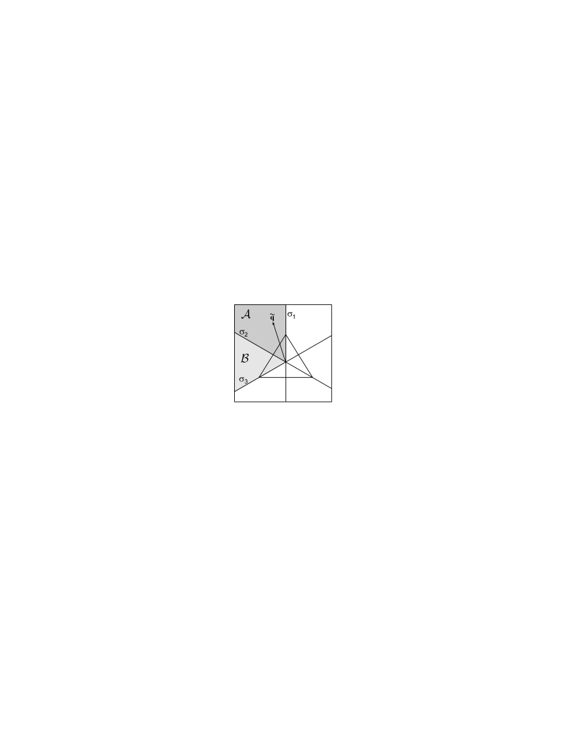
Figure 11: Partition of the set of available wave vectors $\mathbf{q}$. The whole set can be obtained by applying symmetry operations of the $C_{3v}$ group on the subset $\mathcal{A}$.

For the irrep $A_{1}$ the five non-trivial relations of (66) for a given $\mathbf{q}$ allow to restrict the plane wave set $\{\mathbf{q}\}$ to the sixth marked $\mathcal{A}$ in Fig. 11. The set $\{\big{|}A_{1},\tilde{\mathbf{q}}\big{>},\tilde{\mathbf{q}}\in\mathcal{A}\}$ is orthonormal. An analog reasoning applies to the irrep $A_{2}$ based on the five non-trivial relations of (67). For the irrep $E$, (68) yields two non-trivial relations for a given vector $\mathbf{q}$ and a given partner function $j=\pm$. Hence the set $\{\mathbf{q}\}$ may be restricted to a third of its elements, represented by $\mathcal{A}\cup\mathcal{B}$ in Fig. 11. Any two states $\big{|}E,j,\tilde{\mathbf{q}}\big{>}$ and $\big{|}E,j,\mathcal{R}(\sigma_{2})\tilde{\mathbf{q}}\big{>}$ with $\tilde{\mathbf{q}}\in\mathcal{A}$ (and hence $\mathcal{R}(\sigma_{2})\tilde{\mathbf{q}}\in\mathcal{B}$) are non-orthogonal. In order to achieve orthogonality and to use one fixed vector set for all irreps, we introduce the states

$$\begin{split}\big{|}E\pm,\tilde{\mathbf{q}},\chi=1\big{>}&\equiv\big{|}E\pm,\tilde{\mathbf{q}}\big{>}\mp\big{|}E\pm,\sigma_{2}\tilde{\mathbf{q}}\big{>}\\ \big{|}E\pm,\tilde{\mathbf{q}},\chi=2\big{>}&\equiv\big{|}E\pm,\tilde{\mathbf{q}}\big{>}\pm\big{|}E\pm,\sigma_{2}\tilde{\mathbf{q}}\big{>}\\ \end{split}$$ (69)

where $\tilde{\mathbf{q}}\in\mathcal{A}$ and hence $\mathcal{R}(\sigma_{2})\tilde{\mathbf{q}}\in\mathcal{B}$. This definition completes the construction of the one phonon part of the phonon basis (43). The new index $\chi=1,2$ permits the restriction of plane wave vectors to the sixth $\mathcal{A}$ and has the following physical interpretation: All $E$-states with $\chi=1$ involve one plane wave amplitude, whereas the $E$-states with $\chi=2$ mix two different amplitudes (see Fig. 6c).

The canonical transformation relating the symmetrized one-phonon basis to the plane wave basis $\{\big{|}\tilde{\mathbf{q}}\big{>}\}$ results from the definitions (64) and (69) and the normalization relation (65). We find,

$$\left(\begin{array}[]{l}\big{|}A_{1},\tilde{\mathbf{q}}\big{>}\\ \big{|}A_{2},\tilde{\mathbf{q}}\big{>}\\ \big{|}E,+,\tilde{\mathbf{q}},1\big{>}\\ \big{|}E,+,\tilde{\mathbf{q}},2\big{>}\\ \big{|}E,-,\tilde{\mathbf{q}},1\big{>}\\ \big{|}E,-,\tilde{\mathbf{q}},2\big{>}\\ \end{array}\right)=U\left(\begin{array}[]{l}\big{|}\tilde{\mathbf{q}}\big{>}\\ \big{|}\mathcal{R}(\sigma_{2})\tilde{\mathbf{q}}\big{>}\\ \big{|}\mathcal{R}(C^{+}_{3})\tilde{\mathbf{q}}\big{>}\\ \big{|}\mathcal{R}(\sigma_{3})\tilde{\mathbf{q}}\big{>}\\ \big{|}\mathcal{R}(C^{-}_{3})\tilde{\mathbf{q}}\big{>}\\ \big{|}\mathcal{R}(\sigma_{1})\tilde{\mathbf{q}}\big{>}\\ \end{array}\right)\quad\forall\ \tilde{\mathbf{q}}\in\mathcal{A}$$ (70)

with the unitary transformation matrix

$$U=\left(\begin{array}[]{cccccc}\frac{1}{\sqrt{6}}&\frac{1}{\sqrt{6}}&\frac{1}{\sqrt{6}}&\frac{1}{\sqrt{6}}&\frac{1}{\sqrt{6}}&\frac{1}{\sqrt{6}}\\ \frac{1}{\sqrt{6}}&-\frac{1}{\sqrt{6}}&\frac{1}{\sqrt{6}}&-\frac{1}{\sqrt{6}}&\frac{1}{\sqrt{6}}&-\frac{1}{\sqrt{6}}\\ \frac{1}{2}&-\frac{1}{2}&0&0&-\frac{1}{2}&\frac{1}{2}\\ \frac{1}{\sqrt{12}}&\frac{1}{\sqrt{12}}&-\frac{1}{\sqrt{3}}&-\frac{1}{\sqrt{3}}&\frac{1}{\sqrt{12}}&\frac{1}{\sqrt{12}}\\ \frac{1}{2}&\frac{1}{2}&0&0&-\frac{1}{2}&-\frac{1}{2}\\ \frac{1}{\sqrt{12}}&-\frac{1}{\sqrt{12}}&-\frac{1}{\sqrt{3}}&\frac{1}{\sqrt{3}}&\frac{1}{\sqrt{12}}&-\frac{1}{\sqrt{12}}\\ \end{array}\right)$$ (71)

VII.5 $C_{3v}$-Symmetrized Tensor Product Basis

Based on the symmetrized electron basis (42) and the symmetrized phonon basis (43), we shall construct symmetrized product states. The zero-phonon state $\big{|}0\big{>}$ belonging to the irrep $A_{1}$, the symmetrized product states involving zero phonons readily write,

$$\begin{split}\big{|}A_{1};A_{1},\alpha_{e};0\big{>}&\equiv\big{|}A_{1},\alpha_{e}\big{>}\otimes\big{|}0\big{>}\\ \big{|}E\pm;E;0\big{>}&\equiv\big{|}E\pm\big{>}\otimes\big{|}0\big{>}\\ \end{split}$$ (72)

where $n=1,2$ is the electronic energy index inside $A_{1}$. Semicolons separate intrinsic polaron, electron and phonon indices. As for the symmetrized product states involving one phonon, one uses Clebsch-Gordan coefficients,

$$\begin{array}[]{lll}\big{|}A_{1};A_{1},\alpha_{e};A_{1},\tilde{\mathbf{q}}\big{>}&\equiv&\big{|}A_{1},\alpha_{e}\big{>}\otimes\big{|}A_{1},\tilde{\mathbf{q}}\big{>}\\ \big{|}A_{1};E;E,\tilde{\mathbf{q}},\chi\big{>}&\equiv&\frac{1}{\sqrt{2}}\Big{(}\big{|}E+\big{>}\otimes\big{|}E+,\tilde{\mathbf{q}},\chi\big{>}\\ &&+\big{|}E-\big{>}\otimes\big{|}E-,\tilde{\mathbf{q}},\chi\big{>}\Big{)}\\ \big{|}A_{2};A_{1},\alpha_{e};A_{2},\tilde{\mathbf{q}}\big{>}&\equiv&\big{|}A_{1},\alpha_{e}\big{>}\otimes\big{|}A_{2},\tilde{\mathbf{q}}\big{>}\\ \big{|}A_{2};E;E,\tilde{\mathbf{q}},\chi\big{>}&\equiv&\frac{1}{\sqrt{2}}\Big{(}\big{|}E+\big{>}\otimes\big{|}E-,\tilde{\mathbf{q}},\chi\big{>}\\ &&-\big{|}E-\big{>}\otimes\big{|}E+,\tilde{\mathbf{q}},\chi\big{>}\Big{)}\\ \big{|}E\pm;A_{1},\alpha_{e};E,\tilde{\mathbf{q}},\chi\big{>}&\equiv&\big{|}A_{1},\alpha_{e}\big{>}\otimes\big{|}E\pm,\tilde{\mathbf{q}},\chi\big{>}\\ \big{|}E\pm;E;A_{1},\tilde{\mathbf{q}}\big{>}&\equiv&\big{|}E\pm\big{>}\otimes\big{|}A_{1},\tilde{\mathbf{q}}\big{>}\\ \big{|}E\pm;E;A_{2},\tilde{\mathbf{q}}\big{>}&\equiv&\big{|}E\mp\big{>}\otimes\big{|}A_{2},\tilde{\mathbf{q}}\big{>}\\ \big{|}E\pm;E;E,\tilde{\mathbf{q}},\chi\big{>}&\equiv&\frac{1}{\sqrt{2}}\Big{(}\big{|}E+\big{>}\otimes\big{|}E\pm,\tilde{\mathbf{q}},\chi\big{>}\\ &&\mp\big{|}E-\big{>}\otimes\big{|}E\mp,\tilde{\mathbf{q}},\chi\big{>}\Big{)}\end{array}$$

where $\chi=1,2$ is the additional phonon index used for $E$-like one-phonon states.

References

- (1) D. L. Huffaker, G. Park, Z. Zou, O. B. Shchekin, and D. G. Deppe, Appl. Phys. Lett. 73, 2564 (1998).
- (2) S.-W. Lee, K. Hirakawa, and Y. Shimada, Appl. Phys. Lett. 75, 1428 (1999).
- (3) Ch. Santori, M. Pelton, G. Solomon, Y. Dale, and Y. Yamamoto, Phys. Rev. Lett. 86, 1502 (2001).
- (4) M. Pelton, Ch. Santori, J. Vuckovic, B. Zhang, G. Solomon, J. Plant, and Y. Yamamoto, Phys. Rev. Lett. 89, 233602 (2002).
- (5) M. Han, X. Gao, J. Z. Su, and S. Nie, Nature Biotechnology 19, 631 (2001).
- (6) X. Wu, H. Liu, J. Liu, K. Haley, J. Treadway, J. Larson, N. Ge, F. Peale, and M. Bruchez, Nature Biotechnology 21, 41 (2003).
- (7) R. D. Schaller and V. I. Klimov, Phys. Rev. Lett. 92, 186601 (2004).
- (8) F. Klopf, R. Krebs, J. P. Reithmaier, and A. Forchel, IEEE Photon. Technol. Lett. 13 764 (2001).
- (9) D. Loss and D. P. DiVincenzo, Phys. Rev. A 57, 120 (1998).
- (10) U. Bockelmann and G. Bastard, Phys. Rev. B 42, 8947 (1990).
- (11) H. Benisty, C. M. Sotomayor-Torres, and C. Weisbuch, Phys. Rev. B 44, 10945 (1991).
- (12) K. Brunner, U. Bockelmann, G. Abstreiter, M. Walther, G. Böhm, G. Tränkle, and G. Weimann, Phys. Rev. Lett. 69, 3216 (1992).
- (13) U. Bockelmann, Phys. Rev. B 48, 17637 (1993).
- (14) J. Urayama, T. B. Norris, J. Singh, and P. Bhattacharya, Phys. Rev. Lett. 86, 4930 (2001).
- (15) R. Heitz, H. Born, F. Guffarth, O. Stier, A. Schliwa, A. Hoffmann, and D. Bimberg, Phys. Rev. B 64, 241305(R) (2001).
- (16) M. Notomi, M. Naganuma, T. Nishida, T. Tamamura, H. Iwamura, S. Nojima, and M. Okamoto, Appl. Phy. Lett. 58, 720 (1991).
- (17) S. Raymond, S. Fafard, S. Charbonneau, R. Leon, D. Leonard, P. M. Petroff, and J. L. Merz, Phys. Rev. B 52, 17238 (1995).
- (18) T. Inoshita and H. Sakaki, Phys. Rev. B 56, R4355 (1997).
- (19) K. Kral and Z. Khas, Phys. Status Solidi B 208, R5 (1998).
- (20) S. Hameau, Y. Guldner, O. Verzelen, R. Ferreira, G. Bastard, J. Zeman, A. Lemaitre, and J.M. Gerard Phys. Rev. Lett. 83, 4152 (1999).
- (21) O. Verzelen, R. Ferreira, and G. Bastard, Phys. Rev. B 62, R4809 (2000).
- (22) T. Stauber, R. Zimmermann, and H. Castella, Phys. Rev. B 62, 7336 (2000).
- (23) T. Stauber and R. Zimmermann, Phys. Rev. B 73, 115303 (2006).
- (24) R. Ferreira, O. Verzelen, and G. Bastard, Phys. Status Solidi B 238, 575 (2003).
- (25) D. Gammon, E.S. Snow, B.V. Shanabrook, D.S. Katzer, D. Park, Phys. Rev. Lett. 76, 3005 (1996).
- (26) P. Tronc, V.P. Smirnov, K.S. Zhuravlec, Phys. Status Solidi B 241, 2938 (2004).
- (27) E. Kapon, E. Pelucchi, S. Watanabe, A. Malko, M. H. Baier, K. Leifer, B. Dwir, F. Michelini, and M.-A. Dupertuis, Physica E 25, 288 (2004).
- (28) H. Fröhlich, H. Pelzer, and S. Zienau, Philos. Mag. 41, 221 (1950).
- (29) F. Michelini, M.-A. Dupertuis, and E. Kapon, Appl. Phys. Lett. 84, 4086 (2004).
- (30) C. H. Bennett, H. J. Bernstein, S. Popescu, B. Schumacher, Phys. Rev. A 53, 2046 (1996).