Probing Anomalous Longitudinal Fluctuations of the Interacting Bose Gas via Bose-Einstein Condensation of Magnons

Abstract

The emergence of a finite staggered magnetization in quantum Heisenberg antiferromagnets subject to a uniform magnetic field can be viewed as Bose-Einstein condensation of magnons. Using non-perturbative results for the infrared behavior of the interacting Bose gas, we present exact results for the staggered spin-spin correlation functions of quantum antiferromagnets in a magnetic field at zero temperature. In particular, we show that in dimensions $1<D\leq 3$ the longitudinal dynamic structure factor $S_{\parallel}({\bm{q}},\omega)$ describing staggered spin fluctuations in the direction of the staggered magnetization exhibits a critical continuum whose weight can be controlled experimentally by varying the magnetic field.

Because magnons in ordered Heisenberg magnets are bosonic quasi-particles, it is natural to expect that under certain conditions these systems can be used to study general properties of interacting Bose gases, such as the phenomenon of Bose-Einstein condensation (BEC). In fact, the renewed interest in BEC in recent years has also led to considerable activity in the field of magnon BEC Nikuni00 ; Radu05 , which we abbreviate MBEC below.

Experimentally, MBEC has been observed in two different classes of systems. The first are spin-singlet systems Nikuni00 such as TlCuCl₃ or Haldane gap spin chains, where MBEC corresponds to the collapse of the singlet-triplet gap at a critical magnetic field and the emergence of long-range magnetic order for larger fields. The second class of systems, which we shall consider in this work, are easy-plane quantum antiferromagnets (QAFs) such as Cs₂CuCl₄ subject to a magnetic field $h$ perpendicular to the easy plane Radu05 . If $h$ exceeds some critical field $h_{c}$, the ground state is a saturated ferromagnet. For $h<h_{c}$ the $U(1)$-symmetry of the Hamiltonian is spontaneously broken and antiferromagnetic long-range order emerges. At zero temperature, the boson density vanishes at the phase transition so that many-body interactions are not relevant at the zero temperature quantum critical point. However, the finite temperature transition belongs to the same universality class as BEC in the interacting Bose gas. One advantage of studying BEC in magnetic systems is that the magnetic analogon $h_{c}-h$ of the chemical potential can easily be controlled experimentally. Another advantage, which has attracted little attention to date, is that in MBEC the phase of the condensate has a direct physical interpretation as the orientation of the staggered magnetization within the easy plane.

The concept of MBEC has been formulated theoretically many years ago Matsubara56 ; Batyev84 ; Batyev85 ; Affleck90 , where the focus was mainly on the nature of the quantum phase transition. However, even away from the critical point, perturbation theory for the interacting Bose gas is plagued by divergences originating from the gapless dispersion of the Goldstone mode, giving rise to non-analytic behavior of some boson correlation functions Castellani97 ; Weichman88 ; Giorgini92 . Yet, in all physical observables of the Bose gas these divergences cancel, so that they seem to be little more than a mathematical curiosity. Here, we point out that, in contrast to the Bose gas, in MBEC the anomalous behavior arising from the divergences can be directly observed experimentally. We shall exploit recent renormalization group results Castellani97 to obtain the infrared behavior of the staggered spin-spin correlation functions of QAFs in a uniform magnetic field at zero temperature. In particular, we shall show that in dimensions $1<D\leq 3$ the longitudinal part $S_{\parallel}({\bm{q}},\omega)$ of the dynamic structure factor (corresponding to spin-fluctuations parallel to the staggered magnetization) exhibits a critical continuum for small wave-vectors $|{\bm{q}}|$ and frequencies $\omega$, which can be measured via neutron scattering.

We start from the Hamiltonian of the spin-$S$ QAF on a $D$-dimensional hypercubic lattice with $N$ sites and lattice spacing $a$ in a uniform magnetic field in $z$-direction,

$${H}=\frac{1}{2}\sum_{ij}J_{ij}{\bm{S}}_{i}\cdot{\bm{S}}_{j}-h\sum_{i}S^{z}_{i}\;,$$ (1)

where the sums are over all sites of the lattice, and ${\bm{S}}_{i}$ are spin operators with ${\bm{S}}_{i}^{2}=S(S+1)$. We assume nearest neighbor coupling, i.e., $J_{ij}=J>0$ if $i$ and $j$ are nearest neighbors, and $J_{ij}=0$ otherwise. For sufficiently large $h$, the ground state of Eq. (1) is a saturated ferromagnet with magnetization parallel to the field. To obtain the low-lying magnon excitations, we express the spin operators in terms of canonical boson operators $b_{i}$ using the Holstein-Primakoff transformation, $S^{-}_{i}=\sqrt{2S}b_{i}^{\dagger}[1-n_{i}/(2S)]^{1/2}=(S^{+}_{i})^{\dagger}$, $S^{z}_{i}=S-n_{i}$, where $n_{i}=b^{\dagger}_{i}b_{i}$. Expanding the square roots and neglecting terms involving six and more boson operators we obtain ${H}\approx E_{0}+H_{2}+H_{4}$. The constant part is $E_{0}=N[\tilde{J}_{0}S^{2}/2-hS]$, where $\tilde{J}_{0}=\tilde{J}_{\bm{k}=0}$ with $\tilde{J}_{\bm{k}}=\sum_{j}e^{i{\bm{k}}\cdot{\bm{r}}_{j}}J_{ij}$. The quadratic and the quartic contributions to the Hamiltonian are

$$H_{2} = -\frac{S}{2}\sum_{ij}J_{ij}[n_{i}+n_{j}-b^{\dagger}_{i}b_{j}-b^{\dagger}_{j}b_{i}]+h\sum_{i}n_{i},\;\;$$ (2)

$$H_{4} = \frac{1}{4}\sum_{ij}J_{ij}[2n_{i}n_{j}-b_{i}^{\dagger}n_{i}b_{j}-b_{j}^{\dagger}n_{i}b_{i}]\;.$$ (3)

Anticipating antiferromagnetic symmetry breaking, it is convenient to define the Fourier transform in the reduced (antiferromagnetic) Brillouin zone with two branches of magnon operators $b_{\bm{k}\sigma}$ labelled by momenta ${\bm{k}}$ in the reduced zone and $\sigma=\pm$,

$$b_{\bm{k}\sigma}=N^{-1/2}\bigl{[}\sum_{i\in A}e^{-i{\bm{k}}\cdot{\bm{r}}_{i}}b_{i}+\sigma\sum_{i\in B}e^{-i{\bm{k}}\cdot{\bm{r}}_{i}}b_{i}\bigr{]}\;.$$ (4)

Here $i\in A/B$ denotes a summation over the sites of only one of the sublattices $A$ or $B$. The quadratic magnon Hamiltonian is then diagonal, $H_{2}=\sum_{\bm{k}\sigma}(\epsilon_{\bm{k}\sigma}-\mu)b^{\dagger}_{\bm{k}\sigma}b_{\bm{k}\sigma}$, with magnon dispersion $\epsilon_{\bm{k}\sigma}=(\tilde{J}_{0}+\sigma\tilde{J}_{\bm{k}})S$ and $\mu=h_{c}-h$, where $h_{c}=2\tilde{J}_{0}S$. For small wave-vectors $\epsilon_{\bm{k},-}\approx{\bm{k}^{2}}/(2m)$, with effective mass $m=(2JSa^{2})^{-1}$, while the symmetric mode $\epsilon_{\bm{k},+}$ is gapped, $\epsilon_{\bm{k}=0,+}=h_{c}$, so that $\epsilon_{\bm{k}=0,+}-\mu=h$. Note that the gapless mode $\sigma=-1$ describes staggered spin fluctuations.

Since in this work we are interested in the infrared behavior of correlation functions at energy scales smaller than $h$, we shall ignore the gapped mode. To derive the interaction part of the Hamiltonian of the gapless magnons, we substitute Eq. (4) into Eq. (3) and neglect all terms involving the operators $b_{\bm{k},+}$. Defining the field operators $\hat{\psi}_{\bm{k}}=V^{1/2}b_{\bm{k},-}$, where $V=Na^{D}$ is the volume of the system, we obtain for $N\rightarrow\infty$,

$$H = E_{0}+\int_{\bm{k}}(\frac{\bm{k}^{2}}{2m}-\mu)\hat{\psi}_{\bm{k}}^{\dagger}\hat{\psi}_{\bm{k}}$$ (5)

$$+ \frac{1}{2}\int_{\bm{q}}\int_{\bm{k}}\int_{\bm{k}^{\prime}}U_{\bm{q}}\hat{\psi}_{\bm{k}+{\bm{q}}}^{\dagger}\hat{\psi}_{\bm{k}^{\prime}-{\bm{q}}}^{\dagger}\hat{\psi}_{\bm{k}^{\prime}}\hat{\psi}_{\bm{k}}\;,$$

where $\int_{\bm{k}}=\int d^{D}k/(2\pi)^{D}$ and the effective interaction is $U_{\bm{q}}=\Theta(\Lambda_{0}-|{\bm{q}}|)\chi_{0}^{-1}$. Here $\Lambda_{0}\approx a^{-1}$ is an ultraviolet cutoff and $\chi_{0}=(2\tilde{J}_{0}a^{D})^{-1}$ is the leading large-$S$ result for the uniform transverse susceptibility in $x$-direction, which is perpendicular to the staggered magnetization and to the magnetic field. This completes our mapping of the spin system onto an interacting Bose gas.

For $\mu>0$ the field operator $\hat{\psi}_{\bm{k}=0}$ acquires a vacuum expectation value, corresponding to the emergence of long-range antiferromagnetic order. The spin configuration in the ground state is then canted, as shown in Fig. 1.

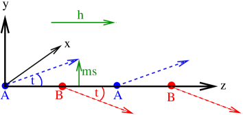
Figure 1: (Color online) Spin configuration in the ground state of a QAF in a uniform magnetic field for $h<h_{c}$. The local moments $\langle{\bm{S}}_{i}\rangle$ are represented by dashed arrows. We choose the coordinate system such that the magnetic field ${\bm{h}}$ points in the $z$-direction and the staggered magnetization $\bm{M}_{s}$ points in the $y$-direction. The sublattices are labelled A and B.

One should keep in mind, however, that Eq. (5) is accurate only for small $\theta$, since otherwise the Bose gas is no longer dilute such that a three-body interaction must be added. However, the qualitative behavior of correlation functions is largely determined by symmetry Castellani97 , so that our results derived below are expected to remain valid also for larger canting angles. Of course, if $\theta$ is not small it is better to quantize the spin operators in a suitably defined tilted basis footnote3 ; Hasselmann06b . For simplicity, we shall focus here on the regime $\theta\ll 1$ where our approach based on the Holstein-Primakoff transformation with quantization axis along the direction of the magnetic field is thus quantitatively accurate for large $S$. Alternatively, we could represent the spin operators in terms of projected bosons Batyev84 ; Batyev85 ; footnote1 which account for all $1/S$ corrections at small $\theta$. However, in the spirit of Ref. [Chakravarty88, ], we take the finite corrections due to higher orders in $1/S$ implicitly into account by expressing our final result in terms of the true spin-wave velocity $c$ and the spin susceptibility $\chi$, which can be obtained from experiments.

To leading order in $1/S$, the classical tilt angle $\theta$ is easily obtained by substituting $\hat{\psi}_{\bm{k}}=(2\pi)^{D}\delta(\bm{k})\psi_{0}+\Delta\hat{\psi}_{\bm{k}}$ in Eq. (5) and demanding that the coefficient of the term linear in $\Delta\hat{\psi}_{\bm{k}}$ vanishes. This yields the well known Popov87 relation $|\psi_{0}|^{2}U_{0}=\mu$. To translate this into a condition for $\theta$, we note from Fig. 1 that for large $S$ the tilt angle is related to the staggered magnetization $M_{s}=V^{-1}\sum_{i}\zeta_{i}\langle S^{y}_{i}\rangle$ via $\theta\approx M_{s}/s$. Here $s=S/a^{D}$ is the spin-density of the saturated magnetic state, and $\zeta_{i}=1$ for $i\in A$ and $\zeta_{i}=-1$ for $i\in B$. Since $M^{2}_{s}=2s|\psi_{0}|^{2}$ to leading order in spin-wave theory, we obtain for large $S$

$$\theta^{2}\approx M_{s}^{2}/s^{2}\approx 2\rho_{0}/s=2(1-h/h_{c})\;,$$ (6)

where $\rho_{0}=|\psi_{0}|^{2}$ is the condensate density. Eq. (6) agrees with the small-$\theta$ expansion of the classical result $\cos\theta=h/h_{c}$ Zhitomirsky98 . To obtain the magnon spectrum for large $S$, we neglect all terms higher than quadratic in the $\Delta\hat{\psi}_{\bm{k}}$. After a Bogoliubov transformation, one finds that for $h<h_{c}$ the magnon spectrum is determined by $\epsilon_{\bm{k}}^{2}=\big{(}\frac{{\bm{k}}^{2}}{2m}\big{)}^{2}+c_{0}^{2}{\bm{k}}^{2}$ which for small $\bm{k}$ yields $\epsilon_{\bm{k}}=c_{0}|{\bm{k}}|+{\cal O}(\bm{k}^{3})$, with the magnetic field dependent spin-wave velocity $c_{0}=\sqrt{\mu/m}=2\sqrt{D}JSa\theta$.

We now focus on the spin-wave interactions, which are relevant in $D\leq 3$. The substitution $\hat{\psi}_{\bm{k}}=(2\pi)^{D}\delta(\bm{k})\psi_{0}+\Delta\hat{\psi}_{\bm{k}}$ generates various terms cubic and quartic in $\Delta\hat{\psi}_{\bm{k}}$ which are rather tedious to work with. A perturbative treatment of these terms is plagued by infrared divergences. However, Ward-identities associated with the $U(1)$-symmetry of the Hamiltonian (5) can be used to obtain the infrared behavior of some correlation functions without resorting to perturbation theory. As pointed out in Ref. Castellani97 , the constraints imposed on the correlation functions by the Ward identities are more transparent if one expresses $\hat{\psi}_{\bm{k}}$ in terms of two real fields, corresponding to transverse and longitudinal fluctuations. Recently we have proposed a similar parameterization of the spin-wave expansion in QAFs Hasselmann06 ; Hasselmann06b , which amounts to expressing the field operator $\hat{\psi}_{\bm{k}}$ in terms of two canonically conjugate hermitian operators $\hat{\Pi}_{\bm{k}}$ and $\hat{\Phi}_{\bm{k}}$ as follows footnote2 ,

$$\hat{\psi}_{\bm{k}}=\rho_{0}^{1/2}\hat{\Pi}_{\bm{k}}+i(4\rho_{0})^{-1/2}\hat{\Phi}_{\bm{k}}\;.$$ (7)

Both fields represent staggered spin fluctuations in the directions perpendicular to the magnetic field, where $\hat{\Pi}_{\bm{k}}$ is transverse and $\hat{\Phi}_{\bm{k}}$ longitudinal with respect to the staggered magnetization. More precisely, in the coordinate system shown in Fig. 1 we have for $S\to\infty$,

$$\hat{\Pi}_{\bm{k}}\approx\frac{1}{M_{s}}\sum_{i}\zeta_{i}e^{-i{\bm{k}}\cdot{\bm{r}}_{i}}S^{x}_{i}\;\;,\;\;\hat{\Phi}_{\bm{k}}\approx\frac{M_{s}}{s}\sum_{i}\zeta_{i}e^{-i{\bm{k}}\cdot{\bm{r}}_{i}}S^{y}_{i}\;.$$ (8)

This equation becomes quantitatively accurate even for finite $S$ in the dilute limit $h\to h_{c}$ which can be shown using projected boson operators footnote1 . The condensed phase corresponds to antiferromagnetic order, $\langle\hat{\Phi}_{\bm{k}}\rangle=(2\pi)^{D}\delta(\bm{k})\phi_{0}$, where $\phi_{0}=M_{s}^{2}/s$ for large $S$. Note that the total density of the Bose gas corresponds in the underlying spin system to $\rho=s-V^{-1}\sum_{i}\langle S^{z}_{i}\rangle$, which vanishes for $h\geq h_{c}$ and satisfies $\rho\ll s$ if $h$ is only slightly smaller than $h_{c}$. Corrections to Eq. (8) would be associated with terms which are of linear or higher order in the boson density and become negligible for $h\to h_{c}$.

The infrared behavior of correlation functions is most conveniently derived within a functional integral approach Popov87 ; Castellani97 . The system is then described in terms of an action $S[\Pi,\Phi]$, which is a functional of $c$-number fields depending on imaginary time $\tau$. Formally, these fields can be obtained from the field operators by substituting $\hat{\Pi}_{\bm{k}}\rightarrow\Pi_{\bm{k}}(\tau)$ and $\hat{\Phi}_{\bm{k}}\rightarrow(2\pi)^{D}\delta(\bm{k})\phi_{0}+\Phi_{\bm{k}}(\tau)$. Introducing the Fourier transforms in frequency space, $\Pi_{K}=\int d\tau e^{i\omega\tau}\Pi_{\bm{k}}(\tau)$ and $\Phi_{K}=\int d\tau e^{i\omega\tau}\Phi_{\bm{k}}(\tau)$, the Gaussian part of the action can be written as

$$S_{0}[\Pi,\Phi] = \frac{1}{2}\int_{K}\Bigr{[}\chi_{0}c_{0}^{2}\bm{k}^{2}\Pi_{-K}\Pi_{K}+\chi_{0}^{-1}\Phi_{-K}\Phi_{K}$$ (9)

$$+\omega(\Pi_{-K}\Phi_{K}-\Phi_{-K}\Pi_{K})\Bigr{]}\;.$$

Here $K=({\bm{k}},i\omega)$ is a collective label for momenta and frequencies, and $\int_{K}=\int\frac{d\omega}{2\pi}\int_{\bm{k}}$. The correlation functions are within Gaussian approximation given by

$$\langle\Pi_{K}\Pi_{K^{\prime}}\rangle_{0} = \delta_{K,-K^{\prime}}\frac{\chi_{0}^{-1}}{\omega^{2}+c_{0}^{2}{\bm{k}}^{2}}\;,$$ (10a)

$$\langle\Pi_{K}\Phi_{K^{\prime}}\rangle_{0} = \delta_{K,-K^{\prime}}\frac{\omega}{\omega^{2}+c_{0}^{2}{\bm{k}}^{2}}\;,$$ (10b)

$$\langle\Phi_{K}\Phi_{K^{\prime}}\rangle_{0} = \delta_{K,-K^{\prime}}\frac{\chi_{0}c_{0}^{2}{\bm{k}}^{2}}{\omega^{2}+c_{0}^{2}{\bm{k}}^{2}}\;,$$ (10c)

where $\delta_{K,-K^{\prime}}=(2\pi)^{D+1}\delta(\omega+\omega^{\prime})\delta({\bm{k}}+{\bm{k}}^{\prime})$. It turns out that the Gaussian approximation is qualitatively correct for the transverse correlation function $\langle\Pi_{K}\Pi_{K^{\prime}}\rangle$ and for the mixed correlation function $\langle\Pi_{K}\Phi_{K^{\prime}}\rangle$, where $\langle\dots\rangle$ denotes the full thermal average. Using the results of Ref. [Castellani97, ], we obtain for the true infrared behavior of these correlation functions

$$\langle\Pi_{K}\Pi_{K^{\prime}}\rangle = \delta_{K,-K^{\prime}}\frac{\chi^{-1}}{\omega^{2}+c^{2}{\bm{k}}^{2}}\;,$$ (11a)

$$\langle\Pi_{K}\Phi_{K^{\prime}}\rangle = \delta_{K,-K^{\prime}}\frac{Z_{\parallel}\omega}{\omega^{2}+c^{2}{\bm{k}}^{2}}\;,$$ (11b)

where $c$ is the renormalized spin-wave velocity, $\chi=M_{s}^{2}\rho/(2smc^{2}\rho_{0})=\chi_{0}Z_{\rho}/Z_{c}^{2}$ is the renormalized transverse susceptibility, and $\rho_{0}$ and $\rho$ are the true condensate density and total density. For convenience we have introduced the dimensionless factors $Z_{\rho}=\rho/\rho_{0}$, $Z_{c}=c/c_{0}$, and $Z_{\parallel}=(mc^{2}/{\rho})d\rho_{0}/d\mu$, all of which approach unity in the classical limit $S\rightarrow\infty$. We emphasize that in dimensions $D\leq 3$ some Feynman diagrams contributing to the above correlation functions are infrared divergent. However, the Ward identities Castellani97 guarantee that all divergences cancel, so that the only difference between the exact results (11a, 11b) and the corresponding approximate expressions (10a, 10b) are finite renormalization factors. The exact results (11a, 11b) depend only on parameters which can be expressed in terms of thermodynamic derivatives.

The important point is now that the Ward identities do not impose similar constraints on the longitudinal correlation function $\langle\Phi_{K}\Phi_{K^{\prime}}\rangle$, which in $D\leq 3$ is dominated by a non-analytic term arising from the re-summation of the leading infrared divergences. Using the results derived in Ref. [Castellani97, ] we obtain

$$\langle\Phi_{K}\Phi_{K^{\prime}}\rangle = \delta_{K,-K^{\prime}}\chi\biggl{[}-Z_{\parallel}^{2}\frac{\omega^{2}}{\omega^{2}+c^{2}{\bm{k}}^{2}}$$ (14)

$$+K_{D+1}\frac{(mc)^{3}}{Z_{\rho}^{3}\rho_{0}}\Biggl{\{}\begin{array}[]{ll}\ln[\frac{(mc)^{2}}{\omega^{2}/c^{2}+{\bm{k}}^{2}}]&\mbox{, $D=3$ }\\ \frac{2}{3-D}[\frac{\omega^{2}}{c^{2}}+{\bm{k}}^{2}]^{\frac{D-3}{2}}&\mbox{, $D<3$ }\end{array}\Biggr{]}\;,$$

where $K_{D}=2^{1-D}\pi^{-D/2}/\Gamma(D/2)$. The non-analytic contribution to the longitudinal correlation function of the interacting Bose gas has first been discussed by Weichman Weichman88 , and later in Ref. [Giorgini92, ]. The field $\phi_{K}$ has thus a finite anomalous dimension and its effective action cannot be approximated by a Gaussian. This reflects the general behavior of systems with broken continuous symmetries where Goldstone modes lead to anomalous longitudinal fluctuations Patashinskii73 ; Chakravarty91 ; Giorgini99 ; Sachdev99b ; Zwerger04 . Note that the magnetic field dependent microscopic momentum scale $mc$ is for large $S$ approximately $mc\approx\sqrt{D}\theta/a$. Using a generalized Ginzburg criterium Castellani97 , we find that the non-analytic corrections in Eq. (14) become important for $|\bm{k}|\lesssim k_{G}$, where $k_{G}\approx mc\,[(mc)^{D}/\rho_{0}]^{\frac{1}{3-D}}$ for $D<3$, and $k_{G}\approx mc\exp[-\rho_{0}/(mc)^{3}]$ for $D=3$.

Even though we have derived Eqs. (11a, 11b) and (14) only for small canting angle $\theta$, they remain valid even for moderate values of $\theta$, as long as three-body interactions are negligible. Using Eqs. (8,14), we find for the longitudinal staggered structure factor for $1<D\leq 3$ and $0<\omega/c\lesssim k_{G}$,

$$S_{\parallel}({\bm{k}},\omega) = \frac{\chi\,s^{2}}{M_{s}^{2}}\Biggl{[}\frac{Z_{\parallel}^{2}}{2}c|{\bm{k}}|\delta(\omega-c|{\bm{k}}|)$$ (15)

$$+ C_{D}\frac{(mc)^{3}}{Z_{\rho}^{3}\rho_{0}}\frac{\Theta(\omega-c|\bm{k}|)}{(\omega^{2}/c^{2}-{\bm{k}}^{2})^{\frac{3-D}{2}}}\Biggr{]}\;,$$

where $C_{D}=K_{D+1}[\pi(3-D)/2]^{-1}\sin[\pi(3-D)/2]$. In particular, $C_{3}=K_{4}=(8\pi^{2})^{-1}$ and $C_{2}=\pi^{-3}$. Eq. (15) is the main result of this work. For small $|{\bm{k}}|\lesssim k_{G}$ the critical continuum represented by the last term in Eq. (15) carries most of the spectral weight: Denoting by $I_{c}$ the contribution from the continuum part in Eq. (15) to the energy integrated spectral weight, and by $I_{\delta}$ the corresponding contribution due to the $\delta$-function, we find $I_{c}/I_{\delta}\propto(k_{G}/|\bm{k}|)\ln(k_{G}/|\bm{k}|)$ for $D=2$ and $I_{c}/I_{\delta}\propto(k_{G}/|\bm{k}|)(mc)^{3}/\rho_{0}$ for $D=3$. In both cases the continuum part dominates for $|\bm{k}|\lesssim k_{G}$. However, in three dimensions $k_{G}\propto\theta\exp[-S/(6\sqrt{3}\theta)]$ is exponentially small for $h\approx h_{c}$ so that the region $|\bm{k}|\lesssim k_{G}$ is difficult to resolve experimentally. On the other hand, in $D=2$ we have $k_{G}\approx 4\sqrt{2}\theta/Sa$ so that in this case the critical continuum should be accessible via neutron scattering at scales $|\bm{k}|\lesssim k_{G}$.

In summary, we have shown that in dimensions $1<D\leq 3$ the longitudinal dynamic structure factor of QAFs subject to a uniform magnetic field exhibits a field-dependent critical continuum as described by Eq. (15) which is closely related to the anomalously large longitudinal fluctuations in the condensed phase of the interacting Bose gas. While in the latter case these fluctuations cannot be directly measured, the magnetic realization of BEC offers a direct experimental access to these fluctuations. Both in $D=2$ and $D=3$ the critical continuum dominates the energy integrated longitudinal structure factor if $|\bm{k}|$ is smaller than the Ginzburg scale $k_{G}$. At least in two-dimensional QAFs the critical continuum should be observable in neutron scattering experiments.

This work was supported by the DFG via FOR 412.

References

- (1) T. Nikuni, M. Oshikawa, A. Oosawa, and H. Tanaka, Phys. Rev. Lett. 84, 5868 (2000); R. Coldea, D. A. Tennant, K. Habicht, P. Smeibidl, C. Woltzers, and Z. Tylczynski, Phys. Rev. Lett. 88, 137203 (2002); M. Matsumoto, B. Normand, T. M. Rice, and M. Sigrist, Phys. Rev. Lett. 89, 077203 (2002); T. M. Rice, Science 298, 760 (2002); Ch. Rüegg, N. Cavadini, A. Furrer, H. U. Güdel, K. Krämer, H. Mutka, A. Wildes, K. Habicht, and P. Vorderwisch, Nature 423, 62 (2003); V. S. Zapf, D. Zocco, B. R. Hansen, M. Jaime, N. Harrison, C. D. Batista, M. Kenzelmann, C. Niedermayer, A. Lacerda, and A. Paduan-Filho, Phys. Rev. Lett. 96, 077204 (2006).
- (2) T. Radu, H. Wilhelm, V. Yushankhai, D. Kovrizhin, R. Coldea, Z. Tylczynski, T. Lühmann, and F. Steglich, Phys. Rev. Lett. 95, 127202 (2005).
- (3) T. Matsubara and H. Matsuda, Prog. Theor. Phys. 16, 569 (1956).
- (4) E. G. Batyev and L. S. Braginskii, Zh. Eksp. Teor. Fiz. 87, 1361 (1984) [Sov. Phys. JETP 60, 781 (1984)].
- (5) E. G. Batyev Zh. Eksp. Teor. Fiz. 89, 308 (1985) [Sov. Phys. JETP 62, 173 (1985)]; S. Gluzman, Z. Phys. B 90, 313 (1993).
- (6) I. Affleck, Phys. Rev. B 41, 6697 (1990); ibid. 43, 3215 (1991).
- (7) C. Castellani, C. Di Castro, F. Pistolesi, and G. C. Strinati, Phys. Rev. Lett. 78, 1612 (1997); F. Pistolesi, C. Castellani, C. Di Castro, and G. C. Strinati, Phys. Rev. B 69, 024513 (2004).
- (8) P. B. Weichman, Phys. Rev. B 38, 8739 (1988).
- (9) S. Giorgini, L. Pitaevskii, and S. Stringari, Phys. Rev. B 46, 6374 (1992).
- (10) Based on a self-consistent treatment of a subset of interaction diagrams, a continuum in the dynamical structure factor was predicted at large magnetic fields and large wavevectors in M. E. Zhitomirsky and A. L. Chernyshev, Phys. Rev. Lett. 82, 4536 (1999). They did however not include the quartic magnon interaction.
- (11) N. Hasselmann, F. Schütz, I. Spremo, and P. Kopietz, cond-mat/0511706, (C. R. Chim., in press).
- (12) The usual hard core boson approach Batyev84 for can be generalized for arbitrary spin by setting , with , see Ref. [Batyev85, ]. To leading order in , this reproduces the interaction term in Eq. (3). In the low-density limit this projected boson approach becomes exact.
- (13) S. Chakravarty, B. I. Halperin, and D. Nelson, Phys. Rev. Lett. 60, 1057 (1988); Phys. Rev. B 39, 2344 (1989).
- (14) V. N. Popov, Functional Integrals and Collective Excitations, (Cambridge University Press, Cambridge, 1987).
- (15) M. E. Zhitomirsky and T. Nikuni, Phys. Rev. B 57, 5013 (1998).
- (16) N. Hasselmann and P. Kopietz, Europhys. Lett. 74, 1067 (2006).
- (17) The normalization in Eq. (7) is chosen to identify with the transverse field of the non-linear -model Hasselmann06 ; Hasselmann06b ; Chakravarty88 . The conjugate field is then fixed by the canonical commutation relation .
- (18) A. Z. Patashinskii and V. L. Pokrovskii, Zh. Eksp. Teor. Fiz. 64, 1445 (1973) [Sov. Phys. JETP 37, 733 (1973)].
- (19) S. Chakravarty, Phys. Rev. Lett. 66, 481 (1991).
- (20) S. Giorgini, L. P. Pitaevskii, and S. Stringari, Phys. Rev. Lett. 80, 5040 (1999).
- (21) S. Sachdev, Phys. Rev. B 59, 14054 (1999).
- (22) W. Zwerger, Phys. Rev. Lett. 92, 027203 (2004).