Chaotic scattering through coupled cavities

Abstract

We study the chaotic scattering through an Aharonov-Bohm ring containing two cavities. One of the cavities has well-separated resonant levels while the other is chaotic, and is treated by random matrix theory. The conductance through the ring is calculated analytically using the supersymmetry method and the quantum fluctuation effects are numerically investigated in detail. We find that the conductance is determined by the competition between the mean and fluctuation parts. The dephasing effect acts on the fluctuation part only. The Breit-Wigner resonant peak is changed to an antiresonance by increasing the ratio of the level broadening to the mean level spacing of the random cavity, and the asymmetric Fano form turns into a symmetric one. For the orthogonal and symplectic ensembles, the period of the Aharonov-Bohm oscillations is half of that for regular systems. The conductance distribution function becomes independent of the ensembles at the resonant point, which can be understood by the mode-locking mechanism. We also discuss the relation of our results to the random walk problem.

I Introduction

Starting from the study of atomic nuclei, chaotic scattering has been a topic of intensive research in a large variety of systems such as atoms, molecules, quantum devices, and microwave cavities CS . A fundamental question to be asked is how much information is reflected in the scattering through random media such as disordered and classically chaotic systems. One of the most remarkable and promising ideas is to introduce the statistical concept into the analysis. The ensemble average over different realizations of the sample is considered to calculate several statistical quantities. A large number of systems exhibit universal behavior determined by the symmetry of the systems. For this situation, random matrix theory (RMT) WD ; Mehta ; GMW has been used to understand the result and has played an important role as a standard analytical tool.

Recently, the experimental stage of the chaotic scattering has been shifted from natural to artificial systems. Typical examples are mesoscopic systems MRWHG ; Beenakker ; Alhassid ; Hacken ; ABG such as quantum dots (QDs) and disordered wires. Recent development of nanotechnology makes it possible to fabricate mesoscopic quantum hybrid systems that could not be realized before and a lot of interesting interference phenomena have been observed under controllable external parameters. Due to the interference of wave functions, a system made from parts such as the QD, lead, and quantum point contact cannot be treated separately. Such systems show new interesting phenomena which are absent in single isolated systems. Typical experimentally fabricated systems are the QD on the Aharonov-Bohm (AB) ring YHMS , the side-coupled QD KASKI , and so on.

The model treated in this paper is two QDs put on the two arms of the AB ring. In this so-called “mesoscopic double slit system,” a lot of interesting phenomena such as the AB oscillations and the Fano effects can be observed by the interference of wave functions transmitting through the two arms GIA ; KK ; KAKI ; NTA . In the context of chaotic scattering, it is interesting to apply the known analysis based on RMT VWZ ; pker ; PEI ; ISS ; randomS ; BB94 ; Brouwer ; FS to the AB ring system. We study how the interference effects appear and the conductance behaves as the function of the controllable parameter such as the magnetic flux through the ring.

Our formulation is rather general and the application of our result is not limited to the QD systems. It is known that microwaves in an irregular shaped cavity behave chaotically and the statistical properties can be described by RMT Stockmann ; HZOAA . Based on the formal analogy between the Helmholtz and Schrödinger equations, the classical waves are simulated as quantum mechanical wave functions. Compared with the mesoscopic systems in nanoscale, the cavity system is easier to fabricate and is ideal for an experimental study. We can also observe the Fano effect in this system RLBKS .

How can we define the statistical model for the hybrid system? For the system of two QDs attached to each arm of the AB ring, Gefen et al. GIA considered the case when each dot has a single regular level. As a simple but nontrivial extension, we treat the case when one of the dots has regular levels and the other has random levels. RMT is applied to the random dot.

This model can be viewed as a mixed system of chaotic and integrable levels. In single dot systems, such structure is employed as an idea to explain anomalous phenomena such as critical statistics KLAA and fractal conductance micolich . It is known in the open QD system that the several specific levels couple with the lead strongly while the other levels couple weakly via strong coupled levels SI . Thus it is too simple to treat the dot as a single random matrix and we need to consider the internal structure more seriously. Although our model is not directly related to such phenomena, it is instructive and useful to consider the present ring system as the situation where the strong and weak couplings coexist. In this system, the regular transmission in the one arm is affected by the random ones in the other arm, and vice versa.

From a point view of RMT, special attention is paid to the universality of the statistical quantities. A natural question to be asked in the present model is how the universal level correlations described by RMT are modified by the regular contribution. Naive expectation is that the effect of the regular levels can be safely removed by the proper scaling (unfolding) BHZ . It is known that the effective theory is written in terms not of the microscopic parameters but of the transmission coefficients VWZ . However, in the present system, the effect is amplified by multiple scatterings through the ring and gives highly nontrivial results.

Now that our model has been described, we must refer to the work by Clerk et al.CWB . They considered many resonant levels in a single dot and RMT was employed for their distribution. The regular component to the S matrix expressing the direct nonresonant path through the dot was used to find the Fano resonances. For each resonance, the Fano parameter $q$ was calculated and the statistical distribution of $q$ was defined over the resonances. On the other hand, in our case, only the single resonant level is present regularly and it is affected by random levels. Thus our attention is fixed on the single regular resonance. To discuss the statistical properties of the transport we must prepare different realizations of the random dot. The ensemble average is defined in terms of such realizations.

The outline of this paper is the following. The AB ring model is defined in Sec.II. We define the random Hamiltonian model in Sec.II.1. A model based on the random S matrix is also defined in Sec.II.2 and the relation to the random Hamiltonian model is discussed. In Sec.III, we calculate the average of the S matrix based on the random Hamiltonian model. As a result the mean part of the conductance is calculated. It is not enough to calculate the conductance including the quantum fluctuation effect and we develop the supersymmetry method Efetov in Sec.IV.1 to calculate the full conductance. The results of the conductance are shown in Sec.IV.2. We also study the AB oscillations in Sec.IV.3 and the Fano effect in Sec.IV.4. The fluctuation effects can be best seen in the conductance distribution functions, which are studied in Sec.V. Since realistic situations are not ideal and phase breaking effect is present HZOAA ; HPMBDH , it is important to consider the dephasing effect theoretically. We consider it in Sec.VI using a simple imaginary-potential model. Section VII is devoted to discussions and conclusions. Part of the results were published in a preliminary report TA .

II Model

II.1 Random Hamiltonian approach

We consider the AB ring system depicted in Fig.1. The upper dot (dot 1) has a single resonant level, and the lower dot (dot 2) has random levels and is treated by RMT.

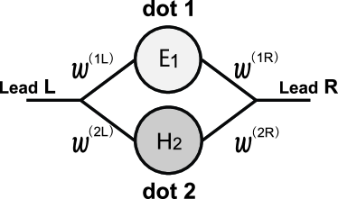
Figure 1: Schematic drawing of our model. Dot 1 with a resonant level $E_{1}$ and dot 2 with a random Hamiltonian $H_{2}$ are connected by leads. $w$ denotes a dot-lead coupling matrix.

It is known from scattering theory that the S matrix of the system is written as Beenakker ; Alhassid ; VWZ ; FS

$$S = 1-2\pi iw^{\dagger}\frac{1}{E-H+i\pi ww^{\dagger}}w$$ (1)

$$= \frac{1-i\pi w^{\dagger}\frac{1}{E^{+}-H}w}{1+i\pi w^{\dagger}\frac{1}{E^{+}-H}w},$$

where $H$ denotes the Hamiltonian matrix for dots and $w$ the dot-lead coupling matrix. $H$ can be written as

$$H=\left(\begin{array}[]{cc}E_{1}&0\\ 0&H_{2}\end{array}\right),$$ (4)

where $E_{1}$ is the fixed energy level for the dot 1 and $H_{2}$ is the random Hamiltonian for the dot 2. The size of $H_{2}$, $N$, is taken to be infinity to find the universal result. We note that the total size of $H$ is $1+N$. It is a straightforward task to extend the size of the upper dot Hamiltonian to arbitrary values and here we consider the minimal size 1. As another simplification, we consider the $2\times 2$ (unitary) matrix $S$, which means that the left and right leads have a single channel, respectively. It is believed that the quantum interference effect becomes maximal in this case BB97 . Then the dot-lead coupling matrix $w$ is the $(1+N)\times 2$ matrix and can be written as

$$w = \left(\begin{array}[]{cc}w^{(1)}\\ w^{(2)}\end{array}\right)=\left(\begin{array}[]{cc}w^{(1L)}&w^{(1R)}\\ w^{(2L)}&w^{(2R)}\end{array}\right)$$ (9)

$$= \left(\begin{array}[]{cc}w^{(1L)}&w^{(1R)}\\ w^{(2L)}_{1}&w^{(2R)}_{1}\\ w^{(2L)}_{2}&w^{(2R)}_{2}\\ \vdots&\vdots\\ w^{(2L)}_{N}&w^{(2R)}_{N}\end{array}\right),$$ (15)

where $(1L)$ refers to the coupling between the dot $1$ and lead $L$, and so on.

The conductance measures the transmission from the left to right lead and is defined by Beenakker ; Alhassid ; VWZ

$$g=\langle|S_{12}|^{2}\rangle,$$ (16)

where $\langle\ \rangle$ denotes the ensemble averaging of the random Hamiltonian $H_{2}$. We employ the Gaussian ensemble Mehta and the probability density is given by

$$P(H)=C\exp\left(-\frac{\pi^{2}}{2N\Delta^{2}}\mbox{tr}\,H^{2}\right),$$ (17)

where $\Delta$ is the mean level spacing, and $C$ is the normalization constant. In the following calculations, we mainly consider unitary symmetry, which means that $H_{2}$ is Hermitian and no additional condition is imposed.

The result of the conductance depends on the choice of the dot-lead coupling $w$. Although this matrix $w$ has $4N$ degrees of freedom, there is no need to specify them completely. After the averaging, the effective degrees of freedom becomes finite. Generally, it is 6 and we restrict our discussion to the special case of 4 (see below).

II.2 Random S matrix approach

Equation (1) is a useful formula to relate the Hamiltonian to the S matrix and can be used for the present coupled system. It is convenient to express the S matrix in terms of the K matrix defined by

$$S=\frac{1-iK}{1+iK}.$$ (18)

$K$ is expressed as the sum of contributions from dot 1 and 2:

$$K=K_{1}+K_{2},$$

$$K=\pi w^{\dagger}\frac{1}{E^{+}-H}w,$$

$$K_{1}=\frac{\pi w^{(1){\dagger}}w^{(1)}}{E^{+}-E_{1}},\;K_{2}=\pi w^{(2){\dagger}}\frac{1}{E^{+}-H_{2}}w^{(2)}.$$ (19)

This simple relation implies the sum rule of the S matrix

$$\frac{1-S}{1+S}=\frac{1-S_{1}}{1+S_{1}}+\frac{1-S_{2}}{1+S_{2}},$$ (20)

where $S_{1}$ ($S_{2}$) is the S matrix for dot 1 (2). It is instructive and useful in the following numerical calculations to derive the explicit representation using the matrix elements. Defining each S matrix elements as

$$S=\left(\begin{array}[]{cc}r&t^{\prime}\\ t&r^{\prime}\end{array}\right),\;S_{i}=\left(\begin{array}[]{cc}r_{i}&t_{i}^{\prime}\\ t_{i}&r_{i}^{\prime}\end{array}\right)\;(i=1,2),$$ (25)

we obtain, for example,

$$t = 4\Bigl{[}t_{1}(1+s_{2}+r_{2}+r_{2}^{\prime})+t_{2}(1+s_{1}+r_{1}+r_{1}^{\prime})\Bigr{]}$$ (26)

$$\times\Bigl{[}9+3(r_{1}+r^{\prime}_{1}+r_{2}+r^{\prime}_{2})+s_{1}+s_{2}$$

$$-3(r_{1}r_{2}+r^{\prime}_{1}r^{\prime}_{2})+(r_{1}r^{\prime}_{2}+r_{2}r^{\prime}_{1})-4(t_{1}t^{\prime}_{2}+t_{2}t^{\prime}_{1})$$

$$-(r_{1}+r^{\prime}_{1})s_{2}-(r_{2}+r^{\prime}_{2})s_{1}+s_{1}s_{2}\Bigr{]}^{-1},$$

where $s_{i}=\det S_{i}=r_{i}r^{\prime}_{i}-t_{i}t^{\prime}_{i}$ ($i=1,2$). Thus the total transmission $t$ is not equal to $t_{1}+t_{2}$, rather including nonlinear effects due to multiple scattering through the ring. Such multiple scattering effects are put together with interference due to random scattering and give highly nontrivial results for the conductance $g=\langle|t|^{2}\rangle$.

Another way of representing the total S matrix is to separate the S matrix of the system into the upper and lower dot parts and the left and right fork parts GIA ; KK . Choosing the fork matrices in a proper way, we can find the same expression of $t$ as in Eq.(26).

The conductance can be calculated by taking the ensemble average over $S_{2}$ determined by the random Hamiltonian $H_{2}$. Instead of doing that, we may disregard the detailed structure of $S_{2}$ and impose randomness directly on $S_{2}$, simulated by the circular ensembles Mehta . It is well known that the random S matrix approach is equivalent to the random Hamiltonian approach if we use the Poisson kernel pker

$$P_{\beta}(S)d\mu_{\beta}(S)\propto\frac{1}{\left|\det\left(1-S\langle S\rangle^{\dagger}\right)\right|^{2\beta+2-\beta}}d\mu_{\beta}(S),$$ (27)

where $d\mu_{\beta}(S)$ denotes the invariant measure for the S matrix and is used as the measure for the circular ensemble. $\beta$ is the index for the universality class. $\beta=1,2,$ and 4 for the unitary, orthogonal, and symplectic case, respectively. $\langle S\rangle$ is the averaged value of S which is treated as an input parameter and is determined by the random Hamiltonian model. The total S matrix is constructed by the sum rule (20) and the conductance is expressed by $|t|^{2}$ where $t$ is given by Eq.(26). By taking the circular ensemble average with the weight $P_{\beta}(S_{2})$, we obtain the conductance $g$ which is the same as that obtained by the random Hamiltonian approach. The equivalence of both approaches was shown in Ref.Brouwer . The random S matrix approach has a great advantage for numerical calculations because there is no need to take the thermodynamic limit $N\to\infty$ and one may consider $2\times 2$ random matrices $S_{2}$.

Alternatively, we can parametrize the S matrix in terms of the K matrix (19). Then the expression of the conductance becomes much simpler than Eq.(26) as we show in Sec.V. The disadvantage of this parametrization is that the K matrix is Hermitian and the matrix elements are not compact, which is inconvenient for the numerical calculation. Thus we employ the S matrix parametrization (26) with compact variables for most of the numerical calculations.

III Averaged S matrix

As we have shown in Eq.(19), the K matrix is written as the sum of the regular (dot 1) and random (dot 2) parts. Thus, to get the averaged K matrix, we may consider the ensemble averaging of the random part. We know from RMT that the averaged Green function for the Gaussian unitary ensemble is given by Mehta

$$\left<\frac{1}{E^{+}-H_{2}}\right>=\frac{\pi}{N\Delta}e^{-iz},$$ (28)

where

$$\cos z=\frac{\pi E}{2N\Delta}.$$ (29)

$N$ is taken to be infinity while $E/\Delta$ is kept finite. Then we have $e^{-iz}\to-i$ and the averaged K matrix is given by

$$\langle K\rangle=\frac{1}{E^{+}-E_{1}}\gamma_{1}-\frac{i\pi}{N\Delta}\gamma_{2},$$ (30)

where $\gamma_{i}=\pi w^{(i){\dagger}}w^{(i)}$ ($i=1,2$). It is important to note that the result depends on the dot-lead couplings $w^{(1,2)}$ through $\gamma_{1,2}$.

For the regular dot, the most general form of $\gamma_{1}$ is

$$\gamma_{1} = \left(\begin{array}[]{cc}\pi w^{(1L)*}w^{(1L)}&\pi w^{(1L)*}w^{(1R)}\\ \pi w^{(1R)*}w^{(1L)}&\pi w^{(1R)*}w^{(1R)}\end{array}\right)$$ (33)

$$= \frac{1}{2}\left(\begin{array}[]{cc}\Gamma_{1L}&\sqrt{\Gamma_{1L}\Gamma_{1R}}e^{-i\phi}\\ \sqrt{\Gamma_{1R}\Gamma_{1L}}e^{i\phi}&\Gamma_{1R}\end{array}\right),$$ (36)

where $\Gamma_{1L}$ ($\Gamma_{1R}$) turns out to be the level width for the left (right) coupling of the dot to the lead and $\phi$ is a phase. We assume the symmetric coupling $\Gamma_{1L}=\Gamma_{1R}$ for simplicity and use

$$\gamma_{1}=\Gamma_{1}\Phi,$$ (37)

where

$$\Phi=\frac{1}{2}\left(\begin{array}[]{cc}1&e^{-i\phi}\\ e^{i\phi}&1\end{array}\right).$$ (40)

This matrix satisfies $\Phi^{2}=\Phi$ and is diagonalized as $\Phi\to{\rm diag}(0,1)$.

On the other hand, for the random dot, the form of $\gamma_{2}$ is slightly complicated. It is written as

$$\gamma_{2}=\left(\begin{array}[]{cc}\pi w^{(2L){\dagger}}w^{(2L)}&\pi w^{(2L){\dagger}}w^{(2R)}\\ \pi w^{(2R){\dagger}}w^{(2L)}&\pi w^{(2R){\dagger}}w^{(2R)}\end{array}\right).$$ (43)

Since $w^{(2L)}$ and $w^{(2R)}$ are $N\times 1$ matrices, we see that the relation $|w^{(2L){\dagger}}w^{(2L)}||w^{(2R){\dagger}}w^{(2R)}|\geq|w^{(2L){\dagger}}w^{(2R)}||w^{(2R){\dagger}}w^{(2L)}|$ holds. The equal sign holds when $w^{(2L)}=w^{(2R)}$ or $N=1$, the latter is the case for $w^{(1)}$. Thus we need the additional parameter for the parametrization of $\gamma_{2}$. Assuming the symmetry of the left and right coupling again, we obtain the form with the level width $\Gamma_{2}$ as

$$\gamma_{2}=\frac{N\Gamma_{2}}{2}\left(\begin{array}[]{cc}1&ae^{i\phi}\\ ae^{-i\phi}&1\end{array}\right).$$ (46)

The parameter $a$ reflects the above mentioned inequality and $0\leq a\leq 1$. We note that the same phase $\phi$ appears in $\gamma_{1}$ and $\gamma_{2}$, but the sign is opposite to each other. This phase affects the transmission part of the S matrix and can be identified with the AB flux through the ring GIA ; KK .

Using this parametrization, we can write

$$\langle K\rangle=\frac{1}{\epsilon}\Phi-\frac{iX}{2}\left(\begin{array}[]{cc}1&ae^{i\phi}\\ ae^{-i\phi}&1\end{array}\right),$$ (49)

where

$$\epsilon=\frac{E-E_{1}}{\Gamma_{1}},\;X=\frac{\pi\Gamma_{2}}{\Delta}.$$ (50)

The energy $\epsilon$ represents the distance from the resonance point and $X$ is the ratio of the level width to the mean level spacing of the dot 2. Thus this model is described by four parameters $\epsilon$, $X$, $a$, and $\phi$.

For the random dot, the elements of the dot-lead coupling $w^{(2)}$ distribute randomly and the summation $\sum_{i=1}^{N}w^{(2L)*}_{i}w^{(2R)}_{i}$ can be small when the random phases of $w^{(2L)}$ and $w^{(2R)}$ almost cancel out. This means $a$ is vanishingly small. On the other hand, the summation can be finite when the left and right dot-lead couplings are correlated mutually. This results in direct nonresonant reaction VWZ . We first discuss the case of $a=0$ for simplicity. The averaged K matrix takes the form

$$\langle K\rangle=\frac{1}{\epsilon}\Phi-\frac{iX}{2}.$$ (51)

The finite-$a$ effect is discussed afterwards.

Now we go back to the S matrix. The averaged S matrix is simply obtained by using the averaged K matrix,

$$\langle S\rangle = \frac{1-\langle K\rangle}{1+\langle K\rangle}$$ (52)

$$= \frac{1-\frac{X}{2}}{1+\frac{X}{2}}-\frac{2i}{\left(1+\frac{X}{2}\right)\left[\left(1+\frac{X}{2}\right)\epsilon+i\right]}\Phi.$$

This is justified by the saddle-point analysis of the nonlinear sigma model described below. We define $g_{0}=|\langle S_{12}\rangle|^{2}$, which is the conductance if we can disregard the quantum fluctuations. It is given by

$$g_{0}=\frac{1}{\left(1+\frac{X}{2}\right)^{2}}\frac{\left(\frac{\Gamma_{1}}{1+\frac{X}{2}}\right)^{2}}{(E-E_{1})^{2}+\left(\frac{\Gamma_{1}}{1+\frac{X}{2}}\right)^{2}}.$$ (53)

The result shows that the level width $\Gamma_{1}$ for the dot 1 and the conductance are renormalized by the factor $1/(1+X/2)$.

For later use, we define the transmission coefficients as

$$T = 1-\langle S\rangle\langle S\rangle^{\dagger}$$

$$= \frac{2X}{\left(1+\frac{X}{2}\right)^{2}}-\frac{2X}{\left(1+\frac{X}{2}\right)^{2}}\frac{\left(\frac{\Gamma_{2}}{1+\frac{X}{2}}\right)^{2}}{(E-E_{1})^{2}+\left(\frac{\Gamma_{2}}{1+\frac{X}{2}}\right)^{2}}\Phi.$$

This matrix can be diagonalized to find the eigenvalues

$$T_{1}=\frac{2X}{\left(1+\frac{X}{2}\right)^{2}},\;T_{2}=\frac{2X}{\left(1+\frac{X}{2}\right)^{2}+\frac{1}{\epsilon^{2}}}.$$ (55)

Note that $0\leq T_{2}\leq T_{1}$, $T_{2}=T_{1}$ at $|E-E_{1}|\to\infty$, and $T_{2}=0$ at $E=E_{1}$. At $X=2$, $T_{1}$ takes the maximum value, $T_{1}=1$, and the transmission through the random dot becomes ideal.

In conclusion of this section, we found the averaged S matrix (52) and the conductance (53). Of course, this is not the final result of the averaged conductance. We just calculated the mean part $g_{0}=|\langle S_{12}\rangle|^{2}$ which is different from the original definition (16). We must examine the fluctuation part $\delta g=g-g_{0}=\langle|S_{12}|^{2}\rangle-|\langle S_{12}\rangle|^{2}$.

IV Conductance

IV.1 Supersymmetry method

We derive the nonlinear sigma model for the coupled system to calculate the fluctuation part of the conductance. According to the supersymmetry method Efetov ; VWZ , the generating function for the product of Green functions $G(E)=1/(E-H+i\pi ww^{\dagger})$ and $G^{\dagger}(E)$ is defined by

$$Z=\int{\cal D}(\bar{\psi},\psi)\exp\Bigl{[}i\bar{\psi}\Bigl{(}E+i\Lambda\pi ww^{\dagger}-H\Bigr{)}\psi\Bigr{]},$$ (56)

where $\psi$ has $4(1+N)$ components coming from supersymmetry (bosons and fermions), retarded-advanced structure, and Hamiltonian space. $\Lambda={\rm diag}(1,-1)$ in retarded-advanced space. Following the standard procedure, we introduce the Hubbard-Stratonovitch field $Q$ to write the averaged generating function as

$$\left<Z\right> = \int{\cal D}Q\exp\biggl{\{}-\mbox{str}\,_{4(1+N)}\ln\biggl{[}E+i\Lambda\pi ww^{\dagger}$$ (59)

$$-\left(\begin{array}[]{cc}E_{1}&0\\ 0&\frac{N\Delta}{\pi}Q\end{array}\right)\biggr{]}-\frac{1}{2}\mbox{str}\,_{4}Q^{2}\biggr{\}},$$

where $Q$ is a 4$\times$4 supermatrix. “str ” denotes supertrace and the subscript indicates the size of superspace. When $w=0$, the saddle-point equation is written down as

$$Q=\frac{N\Delta}{\pi}\frac{1}{E^{+}-\frac{N\Delta}{\pi}Q}.$$ (60)

This is easily solved with the proper boundary condition as

$$Q=e^{-iz\Lambda}=\frac{\pi E}{2N\Delta}-i\Lambda\sqrt{1-\left(\frac{\pi E}{2N\Delta}\right)^{2}}\to-i\Lambda,$$ (61)

where we took the limit $N\to\infty$ keeping $E/\Delta$ finite. As a general solution including the saddle-point manifold, we can write

$$Q=-i\sigma,\;\sigma=V\Lambda\bar{V},$$ (62)

where $V$ is the $4\times 4$ supermatrix and satisfies $V\bar{V}=1$. The symmetry of $V$ is determined in the standard way Efetov .

Now the generating function reads

$$\left<Z\right> = \int{\cal D}\sigma e^{-F},$$

$$F = \mbox{str}\,_{4(1+N)}\ln\left[1+\left(\begin{array}[]{cc}\frac{1}{E-E_{1}}&0\\ 0&\frac{\pi}{N\Delta}Q\end{array}\right)i\Lambda\pi ww^{\dagger}\right]$$ (65)

$$= \mbox{str}\,_{8}\ln\left[1+i\Lambda\left(\frac{1}{E-E_{1}}\gamma_{1}-\frac{i\pi}{N\Delta}\gamma_{2}\sigma\right)\right],$$ (66)

where we assumed $\gamma_{1}=\Gamma_{1}\Phi$ and $\gamma_{2}=N\Gamma_{2}/2$. Since the matrix sizes of $\sigma$ and $\gamma$ are 4 and 2, respectively, the total size of the superspace in the last expression is 8. We finally obtain

$$F = \mbox{str}\,_{8}\ln\left[1+i\left(\frac{1}{\epsilon}\Phi-\frac{iX}{2}\Lambda\right)\sigma\right]$$ (67)

$$= \frac{1}{2}\mbox{str}\,_{8}\ln\left[1+\frac{\frac{T}{2}}{1-\frac{T}{2}}\frac{\Lambda\sigma+\sigma\Lambda}{2}\right].$$

The nonlinear sigma model (67) can be written in terms of the transmission matrix $T$ (LABEL:T) and the microscopic fundamental parameter $X$ does not appear in the expression explicitly. This is a manifestation of the universality Mehta ; GMW ; VWZ .

Equation (67) is for systems with unitary symmetry. In the same way we can derive the nonlinear sigma models for the orthogonal and symplectic symmetry classes. Then $\sigma$ becomes an $8\times 8$ supermatrix and the additional symmetry due to time-reversal invariance is imposed Efetov .

IV.2 Conductance

In the nonlinear sigma model approach, the averaged conductance is calculated by performing the integration of the $\sigma$ matrix. The mean part of the conductance $g_{0}$ in Eq.(53) is easily obtained by neglecting the fluctuation of the $\sigma$ matrix as $\sigma=\Lambda$. To find the fluctuation part of the conductance $\delta g=\langle|S_{12}|^{2}\rangle-|\langle S_{12}\rangle|^{2}$, we must take into account the contribution from the saddle-point manifold parametrized by the $V$ matrix. This calculation is highly complicated and we refer to the Appendix A for details. We finally obtain

$$\delta g = \frac{T_{1}+T_{2}}{4}-\left(\frac{1-\frac{X^{2}}{4}}{2X}\right)\left(\frac{1-\frac{X^{2}}{4}-\frac{1}{\epsilon^{2}}}{2X}\right)$$

$$\times\left(\frac{T_{1}T_{2}}{T_{1}-T_{2}}\right)^{2}\left[\frac{T_{1}+T_{2}}{2}-\left(\frac{T_{1}T_{2}}{T_{1}-T_{2}}\right)\ln\frac{T_{1}}{T_{2}}\right],$$

where $T_{1,2}$ are the eigenvalues of the transmission matrix $T$ given by Eq.(55).

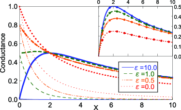
Figure 2: Conductance vs $X=\pi\Gamma_{2}/\Delta$. The thick (thin) lines are analytical results of the total conductance $g$ (mean part $g_{0}$). Inset : Comparison of the analytical (denoted by lines) and numerical (dots) results for the fluctuation part $\delta g=g-g_{0}$.

We first examine the two limiting cases, $|\epsilon|\to\infty$ and $\epsilon=0$. The limit $|\epsilon|\to\infty$ means that dot 1 is detached from the system and the S matrix is given by $S_{1}=1$. In this case, $T_{1}=T_{2}=2X/(1+X/2)^{2}$ and we recover the known result Efetov2

$$\delta g=\frac{T_{1}}{3}+\frac{T_{1}^{2}}{6}.$$ (69)

In the other limit $\epsilon=0$ ($E=E_{1}$) the energy coincides with the level in dot 1 and the perfect transmission through dot 1 is achieved. Then $T_{2}=0$ and we obtain

$$\delta g=\frac{T_{1}}{4}.$$ (70)

We see that Eq.(69) is larger than Eq.(70), which means that the fluctuation effects are reduced as we approach the resonant point. For intermediate values of $\epsilon$, Eq.(LABEL:g1) cannot be written in terms of $T_{1,2}$ only in contrast to Eqs.(69) and (70). This is because the source term to calculate the conductance depends on $\epsilon$ and $X$ explicitly, although the nonlinear sigma model itself can be written in terms of $T$, as shown in the Appendix A.

These results are checked by numerical calculations. We use the formula (26) for the transmission matrix. $S_{1}$ is given by $S_{1}=(1-iK_{1})/(1+iK_{1})$ with $K_{1}=\Phi/\epsilon$, and the random S matrix $S_{2}$ is treated statistically by using the Poisson kernel (27). We take the ensemble average over more than $10^{6}$ samples of the S matrix.

In Fig. 2, $X$ dependence of the conductance is shown for several values of $\epsilon$. $g_{0}$ shows a peak at $X=0$ while $\delta g$ takes a maximum at $X=2$ as shown by the thin lines and the inset in Fig. 2, respectively. As $\epsilon\to\infty$ $g_{0}$ ($\delta g$) is monotonically decreasing (increasing) and the result rapidly approaches Eq.(69). The numerical result agrees with Eq.(LABEL:g1) in a highly accurate way, which shows the equivalence of the random Hamiltonian and random S matrix approach.

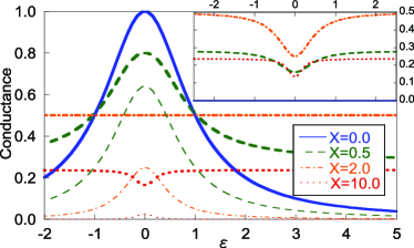
Figure 3: Conductance vs $\epsilon=(E-E_{1})/\Gamma_{1}$. The thick (thin) lines are the total conductance $g$ (the mean part $g_{0}$). Inset : Fluctuation part $\delta g=g-g_{0}$.

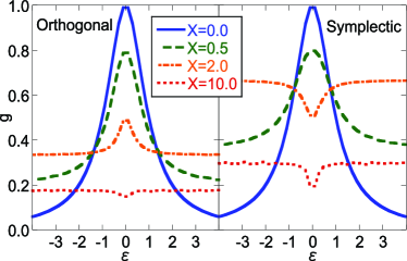
Figure 4: Numerical results of the conductance $g(\epsilon)$ for orthogonal and symplectic ensembles. The result for the symplectic case is normalized to unity.

$\epsilon$ dependence of the conductance is shown in Fig. 3. A resonance peak appears at $\epsilon=0$, reflecting transport through the regular dot 1. This peak structure, however, changes qualitatively as a function of $X$. For small $X$ the peak is convex and the peak height decreases on increasing $X$. When $X=2$, $g$ is independent of $\epsilon$. Increasing $X$ further, we find that the peak turns into an antiresonance and $g$ decreases monotonically. The result for $X=2$ corresponds to that of the circular unitary ensemble because $\langle S_{2}\rangle=0$, and the Poisson kernel $P_{\beta}(S_{2})$ becomes unity. As we see in the inset of Fig.3, $\delta g$ at the resonant point is relatively small and the quantum fluctuation effect smooths the resonance.

For comparison we calculate $g$ as a function of $\epsilon$ for the orthogonal and symplectic ensembles numerically. For the orthogonal case, the Hamiltonian has time-reversal invariance and the matrix elements are real. For symplectic, the Hamiltonian becomes a quaternion real matrix Mehta . The results are shown in Fig.4. When $0<X<2$, the resonance is enhanced (reduced) for the orthogonal (symplectic) ensembles. At $X=2$, the orthogonal ensemble gives a resonance while the symplectic ensemble gives an antiresonance. When $X=10$, we see that antiresonance is reduced (enhanced) for the orthogonal (symplectic) ensemble in contrast to the case of $X<2$.

Away from the resonance, the quantum fluctuation effect becomes larger as the number of degrees of freedom of random variables increases. We note that the number of degrees becomes maximum when $\beta=4$ and minimum when $\beta=1$. We can also see that the conductance at the resonant point is independent of the choice of the ensemble. This result is discussed in detail in Sec.V.

IV.3 Aharonov–Bohm oscillations

For regular ring systems, it is well known that the AB oscillations are observed by applying the magnetic flux through the ring. Since the flux is a tunable parameter it is an important method to control the system. Our interest is how the effect of the AB flux can be observed in the present random system. Can the AB oscillations survive after the random averaging?

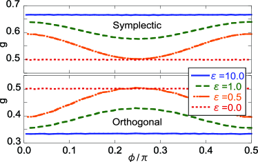
Figure 5: Conductance vs $\phi$ for $X=2$. The lower figure is for the orthogonal ensemble and upper for symplectic. No oscillations are observed for the unitary case.

In systems with unitary symmetry, since the scattering in the random dot randomizes the phase of the amplitude, the result becomes independent of the AB phase $\phi$. This is not the case for the orthogonal and symplectic systems and the oscillations can be observed. However, the period of the oscillation is different from that for regular systems. This can be understood from the expression of the transmission $t$ in Eq.(26). The phase is included in that expression as

$$t=\frac{At_{1}e^{i\phi}+Bt_{2}e^{-i\phi}}{C-D(t_{1}t^{\prime}_{2}e^{2i\phi}+t_{2}t^{\prime}_{1}e^{-2i\phi})},$$ (71)

where $A$, $B$, $C$, and $D$ are phase independent contributions. If we neglect the multiple scattering effect the total transmission is approximated by $t\sim t_{1}e^{i\phi}+t_{2}e^{-i\phi}$. Then the conductance is given by

$$g \sim |t_{1}e^{i\phi}+t_{2}e^{-i\phi}|^{2}$$ (72)

$$= |t_{1}|^{2}+|t_{2}|^{2}+t_{1}t_{2}^{*}e^{2i\phi}+t_{1}^{*}t_{2}e^{-2i\phi}.$$

We see that the third and fourth terms of the right hand side give oscillations with the period $\pi$. However, these terms vanish after the random averaging. The contributions going around the ring twice give oscillations with the period $\pi/2$ and survive after the averaging. Such contributions come from expanding the denominator. Thus, in the orthogonal and symplectic systems, $g$ depends on the AB phase due to the multiple scattering inside the ring. The period of the AB oscillations becomes half of that for the regular systems. This effect can be interpreted as a kind of the Altshuler-Aronov-Spivak effect AAS for cylinder systems. In a ring system, it was discussed in Ref.AAS2 that the period of the oscillation becomes half a flux quantum by the self-averaging effect.

We show the numerical results in Fig.5 for the orthogonal and symplectic ensembles. The period of the oscillations is $\pi/2$ as we discussed above and the difference between these two results is that the conductance becomes minimum (maximum) for orthogonal (symplectic) at $\phi=0$. This can be understood by the standard mechanism of weak localization weakl .

IV.4 Fano effect

The Fano effect is induced by the correlation of the resonant and direct path CWB ; Fano . The direct path can be described by the parameter $a$ in Eq.(46). If we keep this parameter in Eq.(49), the averaged S matrix is given by

$$\langle S\rangle = \frac{1}{\left(1+\frac{1+a}{2}X\right)\left(1+\frac{1-a}{2}X\right)+\left(1+\frac{1-a\cos 2\phi}{2}X\right)\frac{i}{\epsilon}}$$ (75)

$$\times\left(\begin{array}[]{cc}1-\frac{1-a^{2}}{4}X^{2}-\frac{1-a\cos 2\phi}{2}X\frac{i}{\epsilon}&-\frac{i}{\epsilon}e^{-i\phi}-aXe^{i\phi}\\ -\frac{i}{\epsilon}e^{i\phi}-aXe^{-i\phi}&1-\frac{1-a^{2}}{4}X^{2}-\frac{1-a\cos 2\phi}{2}X\frac{i}{\epsilon}\end{array}\right),$$

The mean part of the conductance is derived from this expression as

$$g_{0} = \frac{a^{2}X^{2}}{\left(1+\frac{1+a}{2}X\right)^{2}\left(1+\frac{1-a}{2}X\right)^{2}}$$ (76)

$$\times\frac{\left|\epsilon-\epsilon_{1}+q\Gamma_{1}\right|^{2}}{(E-E_{1})^{2}+\frac{\left(1+\frac{1-a\cos 2\phi}{2}X\right)^{2}}{\left(1+\frac{1+a}{2}X\right)^{2}\left(1+\frac{1-a}{2}X\right)^{2}}\Gamma_{1}^{2}},$$

where $q$ is the Fano parameter

$$q=\frac{ie^{2i\phi}}{aX}.$$ (77)

Thus the Fano effect appears when $a\neq 0$. The additional condition $\phi\neq 0$ is required to obtain a finite real part of $q$. Then the asymmetric conductance form is obtained. At the limit $|E-E_{1}|\to\infty$, $g_{0}$ has a finite contribution in contrast with Eq.(53). This means that there is a direct regular coupling between the left and right leads through the random dot.

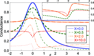
Figure 6: Conductance vs $\epsilon=(E-E_{1})/\Gamma_{1}$ at $a=0.7$ and $\phi=-\pi/8$. The thick (thin) lines are the total conductance $g$ (the mean part $g_{0}$). Inset : Fluctuation part $\delta g=g-g_{0}$. The total conductance $g$ is obtained numerically and the mean part $g_{0}$ is plotted by using Eq.(76)

This Fano effect also appears on $\delta g$. The numerical result in Fig.6 shows that the Fano parameter for $\delta g$ is the same as Eq.(77). Since the antiresonance appears in $\delta g$ as shown in the inset of Fig.3, the asymmetry is opposite to that of $g_{0}$. As a result, the total conductance becomes symmetric. This result means that the Fano effect appears not on $g$ but on the mean part $g_{0}$ and the fluctuation part $\delta g$, respectively. We note that the asymmetric form is obtained when ${\rm Re}\,q\neq 0$. The effect of the imaginary part of $q$ keeps the conductance symmetric. We can conclude that the real part of the Fano parameter does not affect the total conductance. We confirmed that the symmetric conductance is obtained for the orthogonal and symplectic classes as well.

V Conductance distribution functions — mode-locking effect

In the previous section we focused on the averaged conductance. It is well known that disordered systems show strong fluctuation effects, which mean that the square of the conductance and even the higher moments become relevant to characterize the system. To discuss the effects of the fluctuations, here we calculate the conductance distribution function $P(g)=\langle\delta(g-|S_{12}|^{2})\rangle$. We show the analytical results when $\epsilon=0$ which show universality among the ensembles. We also report the numerical results.

The expression of the conductance distribution becomes simpler if we use the K matrix representation as we mentioned in Sec.II.2. $K$ is a Hermite matrix and $K=K_{1}+K_{2}$ with

$$K_{1}=\frac{1}{2\epsilon}\left(\begin{array}[]{cc}1&e^{-i\phi}\\ e^{i\phi}&1\end{array}\right),\;K_{2}=\left(\begin{array}[]{cc}a_{1}&be^{i\phi}\\ b^{\dagger}e^{-i\phi}&a_{2}\end{array}\right).$$ (82)

$a_{1,2}$ are real, and $b$ depends on the universality class and is expressed as

$$b=\left\{\begin{array}[]{cc}b_{0}&\mbox{for}\ \beta=1,\\ b_{0}+ib_{1}&\mbox{for}\ \beta=2,\\ b_{0}+b_{1}e_{1}+b_{2}e_{2}+b_{3}e_{3}&\mbox{for}\ \beta=4,\end{array}\right.$$ (86)

where $b_{0,1,2,3}$ are real and $e_{1,2,3}$ quaternion matrices defined by $e_{j}=i\sigma_{j}$ with the Pauli matrix $\sigma_{j}$ ($j=1,2,3$). The conductance is expressed in this parametrization as

$$g=\left\{\begin{array}[]{cc}\frac{1+4b_{0}\epsilon\cos 2\phi+4|b|^{2}\epsilon^{2}}{\left[b_{0}\cos 2\phi-\frac{a_{1}+a_{2}}{2}+(1-a_{1}a_{2}+|b|^{2})\epsilon\right]^{2}+\left[1+(a_{1}+a_{2})\epsilon\right]^{2}}&\mbox{for}\ \beta=1,\\ \frac{1+4(b_{0}\epsilon\cos 2\phi-b_{1}\sin 2\phi)+4|b|^{2}\epsilon^{2}}{\left[b_{0}\cos 2\phi-b_{1}\sin 2\phi-\frac{a_{1}+a_{2}}{2}+(1-a_{1}a_{2}+|b|^{2})\epsilon\right]^{2}+\left[1+(a_{1}+a_{2})\epsilon\right]^{2}}&\mbox{for}\ \beta=2,\\ \frac{1}{2}\mbox{tr}\,\frac{1+4b_{0}\epsilon\cos 2\phi+4|b|^{2}\epsilon^{2}}{\left[(b_{0}\cos 2\phi-r\sigma_{3}\sin 2\phi)-\frac{a_{1}+a_{2}}{2}+(1-a_{1}a_{2}+|b|^{2})\epsilon\right]^{2}+\left[1+(a_{1}+a_{2})\epsilon\right]^{2}}&\mbox{for}\ \beta=4,\end{array}\right.$$ (90)

where $|b|^{2}=\sum_{i=0}^{\beta-1}b_{i}^{2}$ and $r^{2}=b_{1}^{2}+b_{2}^{2}+b_{3}^{2}$. We note that the conductance for $\beta=4$ is normalized to unity. This expression is averaged by the generalized circular ensemble (Poisson kernel)

$$P_{\beta}(S_{2})d\mu_{\beta}(S_{2})\propto\left\{\frac{1}{\left[\frac{X}{2}+\frac{2}{X}(-a_{1}a_{2}+|b|^{2})\right]^{2}+(a_{1}+a_{2})^{2}}\right\}^{(\beta+2)/2}da_{1}da_{2}\prod_{i=0}^{\beta-1}db_{i},$$ (91)

where we used $\langle S_{2}\rangle=(1-X/2)/(1+X/2)$. The numerical results using the Metropolis algorithm Heermann are shown in Fig.7 at $\phi=0$.

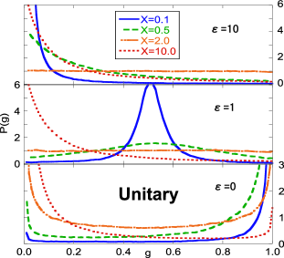
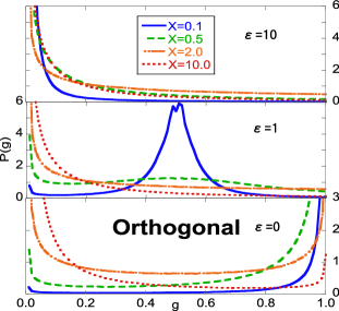
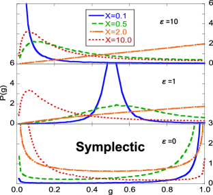
Figure 7: Ensemble dependence of the conductance distribution functions at $\phi=0$. The curves at $\epsilon=0$ are well fitted by the analytical result (95)

The results at large $\epsilon$ are interpreted as the single random dot case. This case was discussed in Ref.PEI using the random Hamiltonian approach and the analytical result for the unitary system was obtained. In the random S matrix approach, the case of the perfect transmission $X=2$ was obtained in Ref.randomS as

$$P(g)=\frac{\beta}{2}g^{-1+\beta/2},$$ (92)

and other cases were discussed in Ref.BB94 . The case of $\epsilon=10$ is enough to find a large-$\epsilon$ result and we find a good agreement with their results.

In the case of $\epsilon=1$, we can clearly see how the random dot significantly affects the distribution function. If we increase $X$, a single peak at small $X$ turns into a broad one and a different peak around $g=0$ is formed at large $X$.

It is interesting to see the results at $\epsilon=0$ which are independent of the choice of the ensemble. In this case, the conductance distribution can be calculated analytically. The conductance is written as

$$g=\frac{1}{1+\left(b_{0}-\frac{a_{1}+a_{2}}{2}\right)^{2}}.$$ (93)

and the distribution function is obtained from the expression

$$P(g)=C\int da_{1}da_{2}\prod_{i=0}^{\beta-1}db_{i}$$

$$\times\delta\left(g-\frac{1}{1+\left(b_{0}-\frac{a_{1}+a_{2}}{2}\right)^{2}}\right)$$

$$\times\left\{\frac{1}{\left[\frac{X}{2}+\frac{2}{X}(-a_{1}a_{2}+|b|^{2})\right]^{2}+(a_{1}+a_{2})^{2}}\right\}^{(\beta+2)/2},$$

where $C$ is the normalization constant. We perform the integrals and obtain

$$P(g)=\frac{1}{\pi\sqrt{g(1-g)}}\frac{1}{\frac{2}{X}(1-g)+\frac{X}{2}g}.$$ (95)

This result agrees with the numerical ones in Fig.7. The reason why this result becomes independent of $\beta$ can be considered as follows. In Eq.(82), all the matrix elements of $K_{1}$ are divergent at $a=0$. When $\phi=0$, this diverging term belongs to the member of the orthogonal ensemble and affects the variables $a_{1,2}$ and $b_{0}$ in the second term $K_{2}$ which are common to all the ensembles. Then the effective modes are locked on those for the orthogonal class and the conductance (93) becomes independent of the rest of the parameters $b_{1,2,3}$.

Equation (95) with $X=2$ appears in the problem of the classical random walk feller and is known as the arcsine law. Consider the one-dimensional classical random walk starting at the origin. The walker can move to either one of its two nearest neighbor sites with the equal probability $p=0.5$. After the $N$-step walk, we count the number of the events which the walker was in the positive axis $M$. Then the distribution function of $g=M/N$ approaches Eq.(95) with $X=2$ as $N\to\infty$. It can be considered that the walker at the positive (negative) direction corresponds to the transmission (reflection) to the left (right) lead in our model. Due to the presence of the resonant path through the dot 1, a particle transmitted through the dot 2 can go to either left or right lead with equal probability. The particle reflected by the dot 2 can go either way as well. Thus the particle entered from a lead forgets where it came from. Such a process can be interpreted as a random-walk-like one and gives the same distribution function. It is interesting that the asymmetric random walk with the probability $p\neq 0.5$ can be described by our model with $X\neq 2$. Since the analytic form is not known in the asymmetric random walk, our result may be useful for understanding the result. It is also known that the same distribution function appears in the problem of the continuous-time quantum walk konno .

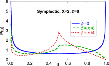
Figure 8: Conductance distribution function of the symplectic system for several values of $\phi$. We set $X=2$ and $\epsilon=0$.

When the phase $\phi$ is finite, $K_{1}$ does not belong to the member of the orthogonal ensemble and the results can depend on the choice of the ensembles. We numerically found that the orthogonal and unitary cases are independent of $\phi$ and the result (95) is kept unchanged. For the symplectic case, we found that the result depends on $\phi$ and Eq.(95) does not maintain anymore. The numerical result for $X=2$ and $\epsilon=0$ is shown in Fig.8. Remarkably, all plotted curves give the averaged conductance $g=0.5$ and the phase dependence appears only for the conductance fluctuations. We also see that plotted curves has a nonanalytic point at around $g=0.5$, which implies a nontrivial mechanism due to the phase coherent effect. It is not clear how this happens and further study is needed to clarify the underlying mechanism.

VI Dephasing

In the Hamiltonian approach, the dephasing effect can be modeled by introducing the imaginary part to the energy

$$\epsilon\to\epsilon+\frac{i}{2\tau}.$$ (96)

This method is equivalent with that of Ref.PEI where the imaginary part of the Hamiltonian was introduced. In the supersymmetry method, this effect can be described by the additional term of the sigma model PEI

$$F_{\tau}=\frac{1}{\Delta\tau}\mbox{str}\,\sigma\Lambda.$$ (97)

This term makes the massless “diffusion” modes on the saddle-point manifold massive and reduces the quantum fluctuations. See the Appendix A for details.

It is well known in the S matrix approach that the dephasing effect can be described by the Büttiker’s voltage probe model Buttiker . A fictitious voltage probe eliminating the phase coherence is attached to the dot and is described by an enlarged S matrix.

Brouwer and Beenakker showed that the voltage-probe model at a certain limit becomes equivalent to the imaginary-potential model and found the modified Poisson kernel in the random S matrix approach BB97 . Here we investigate this limit using the imaginary-potential model. Since the dephasing effect to the regular dot is trivial, we include the effect in the random dot only.

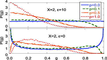
Figure 9: Conductance distribution function for unitary system for several values of $p=1/\Delta\tau$.

In Fig.9, the numerical results of the conductance distribution function using the random Hamiltonian model are shown. We add the dephasing term, $p=1/\Delta\tau$ with the phenomenological dephasing rate $\tau$, to the Hamiltonian. The matrix elements of the dot-lead coupling $w^{(2)}$ are chosen randomly so that there is no direct nonresonant reaction $a=0$. The size of the random Hamiltonian is taken $10^{2}$ and the averaging over $10^{5}$ samples is carried out.

As $p$ increases, the curve transforms into a single peak structure. The peak point corresponds to the mean part of the conductance $g_{0}$, which is close to zero for the upper graph and 0.25 for the lower one. We can conclude that the dephasing effect only affects the fluctuation part. We also confirmed that our numerical result based on the random Hamiltonian agrees with that of the random S matrix model in Ref.BB97 .

VII Conclusions

We have discussed an AB ring system with regular and random cavities. We found that the quantum fluctuation effect plays an important and crucial role and significantly affects the conductance. The main results are summarized as follows: (i) The averaged conductance is divided into two parts. The mean part has the Breit-Wigner resonant form renormalized by random effects. The quantum fluctuation part has an antiresonance form where the quantum effects become minimal at the resonant point. (ii) For the orthogonal and symplectic ensembles, the AB oscillations are found and the period of the oscillations is half a flux quantum. The positive (negative) magnetoconductance are obtained for the orthogonal (symplectic) ensemble because of the multiple reflections inside of the ring. (iii) Depending on the parameter choice, the Fano effect can be observed. This effect appears in the mean and fluctuation parts, respectively, and a symmetric form is obtained for the total conductance. (iv) The conductance distribution functions clearly show the influence of strong fluctuations. The distribution function at the resonant point, Eq.(95), does not depend on the choice of the ensemble, which can be understood by the mode-locking mechanism. The form of the distribution function implies a relation to the random walk problem. (v) The dephasing effect simulated by the imaginary-potential model reduces the fluctuation part only.

The result of the averaged conductance in Fig.3 shows that the total conductance as a function of the energy takes a broad distribution. The form of the total conductance is determined by the competition between the mean (53) and fluctuation (LABEL:g1) parts. At large $X$ we can observe the antiresonance.

Separating the mean and fluctuation parts is crucial to understand the obtained result. For example the Fano effect is found in both parts, while the total conductance, the sum of them, becomes symmetric. We also found that the dephasing effect suppresses the fluctuation part, which means that the cancellation is incomplete and the asymmetric form can be obtained in a system with dephasing.

The most striking result can be seen in the calculation of the conductance distribution function. At the resonant point, the effective modes of the K matrix in Eq.(82) are locked to those for the orthogonal ensemble. Only the orthogonal modes are amplified by the multiple scattering through the ring and we can find the ensemble-insensitive result. This result suggests a possibility of controlling the ensemble dependence of random systems by the resonant singularity embedded in the systems.

Our results for a coupled system show that the nontrivial phenomena which are absent in the single system can be observed in the hybrid system, which opens a new direction for theoretical and experimental studies of chaotic scattering. In this paper we only considered the regular-random coupled system. It is interesting to see more complicated systems such as a random-random system and triple coupled cavities, and so on. A study of the series coupled random dot can be seen, e.g., in Ref.IWZ . To the best of our knowledge, there is no systematic study on the parallel coupled system. It will be discussed in detail in a future publication AT .

Appendix A Calculation of the conductance

We calculate the conductance using the nonlinear sigma model with unitary symmetry, Eq.(67). The first step to do is to represent the conductance as an integral of the $\sigma$ matrix. This is the standard prescription discussed in detail in Ref.VWZ and we have

$$\langle|S_{12}|^{2}\rangle = \biggl{<}\mbox{str}\,\left(k\frac{1+\Lambda}{2}\tilde{K}\frac{1}{1+i\Lambda\tilde{K}}\right)_{12}$$ (98)

$$\times\mbox{str}\,\left(k\frac{1-\Lambda}{2}\tilde{K}\frac{1}{1+i\Lambda\tilde{K}}\right)_{21}\biggr{>}_{F}$$

$$+\biggl{<}\mbox{str}\,\left(k\frac{1+\Lambda}{2}\tilde{K}\frac{1}{1+i\Lambda\tilde{K}}\right)_{11}$$

$$\times\left(k\frac{1-\Lambda}{2}\tilde{K}\frac{1}{1+i\Lambda\tilde{K}}\right)_{22}\biggr{>}_{F},$$

where $k={\rm diag}(1,-1)$ in superspace, $\langle\ \rangle_{F}$ denotes the integration over $\sigma$ with the weight $e^{-F}$, and

$$\tilde{K} = \frac{1}{E-E_{1}}\gamma_{1}-\frac{i\pi}{N\Delta}\gamma_{2}\sigma$$ (99)

$$= \frac{1}{\epsilon}\Phi-\frac{iX}{2}\sigma.$$

In the second line we used $a=0$.

The second step is to parametrize the supermatrix $\sigma$. We use Efetov

$$\sigma=U\sigma_{0}\bar{U},$$

$$\sigma_{0}=\left(\begin{array}[]{cc}\cos\hat{\theta}&i\sin\hat{\theta}\\ -i\sin\hat{\theta}&-\cos\hat{\theta}\end{array}\right)_{\rm RA},$$ (102)

$$U=\left(\begin{array}[]{cc}u&0\\ 0&v\end{array}\right)_{\rm RA},$$ (105)

where

$$\hat{\theta}=\left(\begin{array}[]{cc}i\theta_{B}&0\\ 0&\theta_{F}\end{array}\right)_{\rm BF},$$ (108)

and the integration range is given by $0<\theta_{B}<\infty$ and $0<\theta_{F}<\pi$. $U$ includes the anticommuting Grassmann variables and can be written as

$$u=u_{1}u_{2},$$

$$u_{1}=\exp\left(\begin{array}[]{cc}0&i\eta\\ -i\eta^{*}&0\end{array}\right)_{\rm BF},$$ (111)

$$u_{2}=\left(\begin{array}[]{cc}\mbox{e}^{i\varphi_{1}}&0\\ 0&\mbox{e}^{i\varphi_{2}}\end{array}\right)_{\rm BF},$$ (114)

$$v=\exp\left(\begin{array}[]{cc}0&\kappa\\ -\kappa^{*}&0\end{array}\right)_{\rm BF},$$ (117)

where $\eta$ and $\chi$ are Grassmann variables and the range of the real variables $\varphi_{1,2}$ is given by $0<\varphi_{1,2}<2\pi$. The invariant measure of this parametrization is

$${\cal D}\sigma = Cd\theta_{B}d\theta_{F}d\varphi_{1}d\varphi_{2}d\eta d\eta^{*}d\kappa d\kappa^{*}$$ (118)

$$\times\frac{\sinh\theta_{B}\sin\theta_{F}}{(\cosh\theta_{B}-\cos\theta_{F})^{2}},$$

where $C$ is the normalization constant. In this parametrization, we can write

$$e^{-F}=\frac{\left[1-\frac{T_{1}}{2}(1-\cos\theta_{F})\right]\left[1-\frac{T_{2}}{2}(1-\cos\theta_{F})\right]}{\left[1+\frac{T_{1}}{2}(\cosh\theta_{B}-1)\right]\left[1+\frac{T_{2}}{2}(\cosh\theta_{B}-1)\right]}.$$

The last step is to carry out the integrations. This calculation is cumbersome although it is a straightforward task. The first term in Eq.(98) includes the mean part $g_{0}$. It is easily obtained by substituting $\sigma=\Lambda$. The fluctuation correction is obtained from the integral

$$\frac{1}{16}\int_{1}^{\infty}ds_{1}\int_{-1}^{1}dse^{-F}$$

$$\times\biggl{|}T_{1}\frac{1-\frac{T_{1}}{2}\left(1+\frac{X}{2}\right)}{\left[1+\frac{T_{1}}{2}(s_{1}-1)\right]\left[1-\frac{T_{1}}{2}(1-s)\right]}$$

$$-T_{2}\frac{1-\frac{T_{2}}{2}\left[1+\frac{X}{2}+\frac{2}{X}\left(\frac{1}{\epsilon^{2}}+\frac{i}{\epsilon}\right)\right]}{\left[1+\frac{T_{2}}{2}(s_{1}-1)\right]\left[1-\frac{T_{2}}{2}(1-s)\right]}\biggr{|}^{2}.$$ (120)

In the same way, the second term in Eq.(98) is reduced to

$$\frac{1}{16}\int_{1}^{\infty}ds_{1}\int_{-1}^{1}ds\frac{1}{(s_{1}-s)^{2}}e^{-F}$$

$$\times\Biggl{\{}\left[\frac{T_{1}}{1+\frac{T_{1}}{2}(s_{1}-1)}+\frac{T_{2}}{1+\frac{T_{2}}{2}(s_{1}-1)}\right]^{2}(s_{1}^{2}-1)$$

$$+\left[\frac{T_{1}}{1-\frac{T_{1}}{2}(1-s)}+\frac{T_{2}}{1+\frac{T_{2}}{2}(1-s)}\right]^{2}(1-s^{2})\Biggr{\}}.$$

(121)

We note that these expressions are obtained after integrating the Grassmann variables and changing the variables as $s_{1}=\cosh\theta_{B}$ and $s=\cos\theta_{F}$. A careful manipulation is required to carry out the remaining integrals. After lengthy calculations we can obtain Eq.(LABEL:g1).

It is a straightforward task to include the dephasing effect described by the dephasing term (97). In the present parametrization, it can be written as

$$F_{\tau}=\frac{2}{\Delta\tau}(s_{1}-s),$$ (122)

and is incorporated in the integrals in Eqs.(120) and (121) as $e^{-F_{\tau}}$. Although we do not show the analytical result explicitly, it is not difficult to carry out the integrals. At the limit $|E-E_{1}|\to\infty$, we can find the result of Ref.PEI .

References

- (1) For a recent review, see Y.V. Fyodorov, T. Kottos, and H.-J. Stöckmann, J. Phys. A 38, 10433 (2005).
- (2) E.P. Wigner, Ann. Math. 53, 36 (1951); F.J. Dyson, J. Math. Phys. 3, 140 (1962); 3, 157 (1962); 3, 166 (1962).
- (3) M.L. Mehta, Random Matrices, 3rd ed. (Academic, New York, 2004).
- (4) T. Guhr, A. Müller-Groeling, and H.A. Weidenmüller, Phys. Rep. 299, 189 (1998).
- (5) C.M. Marcus, A.J. Rimberg, R.M. Westervelt, P.F. Hopkins, and A.C. Gossard, Phys. Rev. Lett. 69, 506 (1992).
- (6) C.W.J. Beenakker, Rev. Mod. Phys. 69, 731 (1997).
- (7) Y. Alhassid, Rev. Mod. Phys. 72, 895 (2000).
- (8) G. Hackenbroich, Phys. Rep. 343, 463 (2001).
- (9) I.L. Aleiner, P.W. Brouwer, and L.I. Grazman, Phys. Rep. 358, 309 (2002).
- (10) A. Yacoby, M. Heiblum, D. Mahalu, and H. Shtrikman, Phys. Rev. Lett. 74, 4047 (1995).
- (11) K. Kobayashi, H. Aikawa, A. Sano, S. Katsumoto, and Y. Iye, Phys. Rev. B 70, 035319 (2004).
- (12) Y. Gefen, Y. Imry, and M.Ya. Azbel, Phys. Rev. Lett. 52, 129 (1984).
- (13) B. Kubala and J. König, Phys. Rev. B 65, 245301 (2002); 67, 205303 (2003).
- (14) K. Kobayashi, H. Aikawa, S. Katsumoto, and Y. Iye, Phys. Rev. Lett. 88, 256806 (2002); Phys. Rev. B 68, 235304 (2003).
- (15) T. Nakanishi, K. Terakura, and T. Ando, Phys. Rev. B 69, 115307 (2004).
- (16) J.J.M. Verbaarschot, H.A. Weidenmüller, and M.R. Zirnbauer, Phys. Rep. 129, 367 (1985).
- (17) L.K. Hua, Harmonic Analysis of Functions of Several Complex Variables in the Classical Domains (American Mathematical Society, Providence, 1963); P.A. Mello, P. Pereyra, and T.H. Seligman, Ann. Phys. (N.Y.) 161, 254 (1985); P.A. Mello and N. Kumar, Quantum Transport in Mesoscopic Systems (Oxford University Press, Oxford, 2004).
- (18) V.N. Prigodin, K.B. Efetov, and S. Iida, Phys. Rev. Lett. 71, 1230 (1993); Phys. Rev. B 51, 17223 (1995).
- (19) F.M. Izrailev, D. Saher, and V.V. Sokolov, Phys. Rev. E 49, 130 (1994).
- (20) H.U. Baranger and P.A. Mello, Phys. Rev. Lett. 73, 142 (1994); R.A. Jalabert, J.-L. Pichard, and C.W.J. Beenakker, Europhys. Lett. 27, 255 (1994).
- (21) P.W. Brouwer and C.W.J. Beenakker, Phys. Rev. B 50, R11263 (1994).
- (22) P.W. Brouwer, Phys. Rev. B 51, 16878 (1995).
- (23) Y.V. Fyodorov and H.-J. Sommers, J. Math. Phys. 38, 1918 (1997); J. Phys. A 36, 3303 (2003).
- (24) H.-J. Stöckmann, Quantum Chaos: An Introduction (Cambridge University Press, Cambridge, U.K., 1999).
- (25) S. Hemmady, X. Zheng, E. Ott, T.M. Antonsen, and S.M. Anlage, Phys. Rev. Lett. 94, 014102 (2005); S. Hemmady, X. Zheng, J. Hart, T.M. Antonsen, Jr., E. Ott, and S.M. Anlage, Phys. Rev. E 74, 036213 (2006).
- (26) S. Rotter, F. Libisch, J. Burgdörfer, U. Kuhl, and H.-J. Stöckmann, Phys. Rev. E 69, 046208 (2004).
- (27) V.E. Kravtsov, I.V. Lerner, B.L. Altshuler, and A.G. Aronov, Phys. Rev. Lett. 72, 888 (1994).
- (28) A.P. Micolich et al., Phys. Rev. Lett. 87, 036802 (2001).
- (29) P.G. Silvestrov and Y. Imry, Phys. Rev. Lett. 85, 2565 (2000).
- (30) E. Brézin, S. Hikami, and A. Zee, Phys. Rev. E 51, 5442 (1995).
- (31) A.A. Clerk, X. Waintal, and P.W. Brouwer, Phys. Rev. Lett. 86, 4636 (2001).
- (32) K.B. Efetov, Adv. Phys. 32, 53 (1983); Supersymmetry in Disorder and Chaos (Cambridge University Press, Cambridge, U.K., 1997).
- (33) A.G. Huibers, S.R. Patel, C.M. Marcus, P.W. Brouwer, C.I. Duruöz, and J.S. Harris, Jr., Phys. Rev. Lett. 81, 1917 (1998).
- (34) K. Takahashi and T. Aono, Phys. Rev. B 74, 041311(R) (2006).
- (35) P.W. Brouwer and C.W.J. Beenakker, Phys. Rev. B 55, 4695 (1997).
- (36) K.B. Efetov, Phys. Rev. Lett. 74, 2299 (1995).
- (37) B.L. Al’tshuler, A.G. Aronov, and B.Z. Spivak, Pis’ma Zh. Eksp. Teor. Fiz. 33, 101 (1981) [JETP Lett. 33, 94 (1981)]; D.Yu. Sharvin and Yu.V. Sharvin, ibid. 34, 285 (1981) [ibid. 34, 272 (1981)]; B.L. Al’tshuler, A.G. Aronov, B.Z. Spivak, D.Yu. Sharvin, and Yu.V. Sharvin, ibid. 35, 476 (1982) [ibid. 35, 588 (1982)].
- (38) J.P. Carini, K.A. Muttalib, and S.R. Nagel, Phys. Rev. Lett. 53, 102 (1984); M. Murat, Y. Gefen, and Y. Imry, Phys. Rev. B 34, 659 (1986); see also Y. Imry, Introduction to Mesoscopic Physics (Oxford University Press, Oxford, 1997).
- (39) For a review, see S. Chakravarty and A. Schmid, Phys. Rep. 140, 193 (1986).
- (40) U. Fano, Phys. Rev. 124, 1866 (1961).
- (41) See for example, D.W. Heermann, Computer Simulation Methods in Theoretical Physics (Springer-Verlag, Berlin, 1986)
- (42) W. Feller, An Introduction to Probability Theory and Its Applications, 3rd ed. (Wiley, New York, 1968).
- (43) N. Konno, Phys. Rev. E 72, 026113 (2005).
- (44) M. Büttiker, Phys. Rev. B 33, 3020 (1986); IBM J. Res. Dev. 32, 63 (1988).
- (45) S. Iida, H.A. Weidenmüller, and J.A. Zuk, Phys. Rev. Lett. 64, 583 (1990); Ann. Phys. (N.Y.) 200, 219 (1990).
- (46) T. Aono and K. Takahashi (unpublished).