Dielectric function, screening, and plasmons in 2D graphene

Abstract

The dynamical dielectric function of two dimensional graphene at arbitrary wave vector $q$ and frequency $\omega$, $\epsilon(q,\omega)$, is calculated in the self-consistent field approximation. The results are used to find the dispersion of the plasmon mode and the electrostatic screening of the Coulomb interaction in 2D graphene layer within the random phase approximation. At long wavelengths ($q\rightarrow 0$) the plasmon dispersion shows the local classical behavior $\omega_{cl}=\omega_{0}\sqrt{q}$, but the density dependence of the plasma frequency ($\omega_{0}\propto n^{1/4}$) is different from the usual 2D electron system ($\omega_{0}\propto n^{1/2}$). The wave vector dependent plasmon dispersion and the static screening function show very different behavior than the usual 2D case. We show that the intrinsic interband contributions to static graphene screening can be effectively absorbed in a background dielectric constant.

I introduction

There has been a great deal of recent interest in the electronic properties of two dimensional (2D) graphene, a single-layer graphite sheet, both theoretically and experimentally Geim ; Kim . The main difference of 2D graphene compared with other (mostly semiconductor-based) 2D materials is the electronic energy dispersion. In conventional 2D systems, the electron energy with an effective mass $m^{*}$ depends quadratically on the momentum, but in graphene, the dispersions of electron and hole bands are linear near K, K’ points of the Brillouin zone. Because of the different energy band dispersion, screening properties in graphene exhibit significantly different behavior from the conventional 2D systems rmp . The screening of Coulomb interaction induced by many body effects is one of the most important fundamental quantities for understanding many physical properties. For example, dynamical screening determines the elementary excitation spectra and the collective modes of the electron system, and static screening determines transport properties through screened Coulomb carrier scattering by charged impurities. In this paper, we theoretically obtain the (dynamical and static) screening behavior of 2D graphene by calculating, for the first time, the polarizability and the dielectric function within the self-consistent field approximation (i.e. random-phase-approximation (RPA)) for gated-2D graphene free carrier systems. We apply our theory to calculate the 2D graphene plasmon dispersion and the static screening function, finding some interesting qualitative differences between graphene and the extensively studied 2D electron systems based on semiconductor heterostructures and MOSFETs.

In this paper, we calculate the dielectric function of graphene at arbitrary wave vector $q$ and frequency $\omega$, $\epsilon(q,\omega)$, within RPA, in which each electron is assumed to move in the self-consistent field arising from the external field plus the induced field of all electrons. This is the model which leads to the famous Lindhard dielectric function for a three-dimensional (3D) Lindhard1 and 2D Lindhard2 electron gas. One of the immediate theoretical consequences of the dielectric function is that its zeros give the wave vector dependent plasmon mode, $\omega_{pl}(q)$, which is a fundamental elementary excitation and a collective density oscillation mode. Using the theoretical dielectric function we provide the plasmon mode dispersion both for single-layer and bilayer graphene. Another important consequence of the dielectric function is the static screening function which can be obtained as the static limit $\omega\rightarrow 0$ of the dielectric function, describing the electrostatic screening of the electron-electron, electron-lattice, and electron-impurity interactions.

II Polarizability: $\Pi^{+}$ and $\Pi^{-}$

The electron dynamics in 2D graphene is modeled by a chiral Dirac equation, which describes a linear relation between energy and momentum. The corresponding kinetic energy of graphene for 2D wave vector k is given by (we use $\hbar=1$ throughout this paper)

$$\epsilon_{s{\bf k}}=s\gamma|{\bf k}|,$$ (1)

where $s=\pm 1$ indicate the conduction (+1) and valence ($-1$) bands, respectively, and $\gamma$ is a band parameter (essentially the 2D Fermi velocity, which is a constant for graphene instead of being density dependent). The corresponding density of states (DOS) is given by $D(\epsilon)=g_{s}g_{v}|\epsilon|/(2\pi\gamma^{2})$, where $g_{s}=2$, $g_{v}=2$ are the spin and valley degeneracies, respectively. The Fermi momentum ($k_{F}$) and the Fermi energy ($E_{F}$) of 2D graphene are given by $k_{F}=(4\pi n/g_{s}g_{v})^{1/2}$ and $E_{F}=\gamma k_{F}$ where $n$ is the 2D carrier (electron or hole) density. For the sake of completeness, we also mention that the dimensionless Wigner-Seitz radius ($r_{s}$), which measures the ratio of the potential to the kinetic energy in an interacting quantum Coulomb system Lindhard1 , is given in doped 2D graphene by $r_{s}=(e^{2}/\kappa\gamma)(4/g_{s}g_{v})^{1/2}$ where $\kappa$ is the background lattice dielectric constant of the system. We note in the passing the curious fact that the dimensionless $r_{s}$ parameter is a constant in graphene unlike in the usual 2D ($r_{s}\sim n^{-1/2}$) and 3D ($r_{s}\sim n^{-1/3}$) electron liquids, where $r_{s}$ (and therefore interaction effects) increases with decreasing carrier density. The constancy of $r_{s}$ in graphene arises trivially from the relativistic Dirac-like nature of the free carrier graphene dynamics implying that the ‘relativistic’ effective mass, $m_{c}=E_{F}/\gamma^{2}$, depends on carrier density precisely as $\sqrt{n}$ cancelling out the corresponding $\sqrt{n}$ term in the potential energy. Equivalently, $r_{s}$ here is just the “effective fine structure constant” for graphene, with a value of $r_{s}\sim 0.5$ assuming $g_{s}=g_{v}=2$ and $\kappa=4$ (using SiO₂ as the substrate material). This small (and constant) value of graphene $r_{s}$ indicates it to be a weakly interacting system for all carrier densities, making RPA an excellent approximation in graphene since RPA is asymptotically exact in the $r_{s}\ll 1$ limit.

In the RPA, the dynamical screening function (dielectric function) becomes

$$\varepsilon(q,\omega)=1+v_{c}(q)\Pi(q,\omega),$$ (2)

where $v_{c}(q)=2\pi e^{2}/\kappa q$ is the 2D Coulomb interaction, and $\Pi(q,\omega)$, the 2D polarizability, is given by the bare bubble diagram

$$\Pi(q,\omega)=-\frac{g_{s}g_{v}}{L^{2}}\sum_{{\bf k}ss^{\prime}}\frac{f_{s{\bf k}}-f_{s^{\prime}{\bf k}^{\prime}}}{\omega+\epsilon_{s{\bf k}}-\epsilon_{s^{\prime}{\bf k}^{\prime}}+i\eta}F_{ss^{\prime}}({\bf k},{\bf k}^{\prime}),$$ (3)

where ${\bf k}^{\prime}={\bf k}+{\bf q}$, $s,s^{\prime}=\pm 1$ denote the band indices and $F_{ss^{\prime}}({\bf k},{\bf k}^{\prime})$ is the overlap of states and given by $F_{ss^{\prime}}({\bf k},{\bf k}^{\prime})=(1+ss^{\prime}\cos\theta)/2$, where $\theta$ is the angle between ${\bf k}$ and ${\bf k}^{\prime}$, and $f_{sk}$ is the Fermi distribution function, $f_{s{\bf k}}=[\exp\{\beta(\epsilon_{s{\bf k}}-\mu)\}+1]^{-1}$, with $\beta=1/k_{B}T$ and $\mu$ the chemical potential. After performing the summation over $ss^{\prime}$ we can rewrite the polarizability as

$$\Pi(q,\omega)=\Pi^{+}(q,\omega)+\Pi^{-}(q,\omega),$$ (4)

where

$$\Pi^{+}(q,\omega)=-\frac{g_{s}g_{v}}{2L^{2}}\sum_{k}\left[\frac{[f_{{\bf k}+}-f_{{\bf k}^{\prime}+}](1+\cos\theta_{kk^{\prime}})}{\omega+\epsilon_{{\bf k}+}-\epsilon_{{\bf k}^{\prime}+}+i\eta}\right.$$ (5)

$$+ \left.\frac{f_{{\bf k}+}(1-\cos\theta_{kk^{\prime}})}{\omega+\epsilon_{{\bf k}+}-\epsilon_{{\bf k}^{\prime}-}+i\eta}-\frac{f_{{\bf k}^{\prime}+}(1-\cos\theta_{kk^{\prime}})}{\omega+\epsilon_{{\bf k}-}-\epsilon_{{\bf k}^{\prime}+}+i\eta}\right],$$

and

$$\Pi^{-}(q,\omega)=-\frac{g_{s}g_{v}}{2L^{2}}\sum_{k}\left[\frac{[f_{{\bf k}-}-f_{{\bf k}^{\prime}-}](1+\cos\theta_{kk^{\prime}})}{\omega+\epsilon_{{\bf k}-}-\epsilon_{{\bf k}^{\prime}-}+i\eta}\right.$$ (6)

$$+ \left.\frac{f_{{\bf k}-}(1-\cos\theta_{kk^{\prime}})}{\omega+\epsilon_{{\bf k}-}-\epsilon_{{\bf k}^{\prime}+}+i\eta}-\frac{f_{{\bf k}^{\prime}-}(1-\cos\theta_{kk^{\prime}})}{\omega+\epsilon_{{\bf k}+}-\epsilon_{{\bf k}^{\prime}-}+i\eta}\right].$$

For intrinsic (i.e. undoped or ungated with $n$ and $E_{F}$ both being zero) graphene, in which the conduction band is empty and the valence band is fully occupied at zero temperature (i.e. $E_{F}=0$), we have $f_{{\bf k}+}=0$ and $f_{{\bf k}-}=1$. Then the polarizability becomes $\Pi(q,\omega)=\Pi^{-}(q,\omega)$, which has been previously obtained in the renormalization group approach Guinea . Recently $\Pi^{-}(q,\omega)$ has been reconsidered to discuss screening effects of Coulomb interaction in intrinsic graphene khve . In general, $\Pi^{+}(q,\omega)$ does not vanish for most systems because the Fermi energy is typically located in the conduction or the valence band. But graphene is a most peculiar zero-gap semiconductor system where $E_{F}=0$ in the intrinsic undoped situation. In the doped or gated situation $n$, $E_{F}\neq 0$ in graphene, and now $\Pi^{+}$ is finite. In the following we provide the zero temperature polarizability in the doped or gated case where the Fermi energy is not zero.

By introducing the dimensionless quantities $x=q/k_{F}$ and $\nu=\omega/E_{F}$, and $\tilde{\Pi}(q,\omega)=\Pi(q,\omega)/D_{0}$ where $D_{0}\equiv D(E_{F})=(g_{s}g_{v}n/\pi)^{1/2}/\gamma$ is the DOS at Fermi energy, we have

$$\tilde{\Pi}^{+}(x,\nu)=\tilde{\Pi}^{+}_{1}(x,\nu)\theta(\nu-x)+\tilde{\Pi}^{+}_{2}(x,\nu)\theta(x-\nu),$$ (7)

where the real parts of the polarizability are given

$${\rm{Re}}\tilde{\Pi}^{+}_{1}(x,\nu) = 1-\frac{1}{8\sqrt{\nu^{2}-x^{2}}}\left\{f_{1}(x,\nu)\theta(|2+\nu|-x)\right.$$ (8)

$$+ {\rm{sgn}}(\nu-2+x)f_{1}(x,-\nu)\theta(|2-\nu|-x)$$

$$+ \left.f_{2}(x,\nu)[\theta(x+2-\nu)+\theta(2-x-\nu)]\right\}$$

$${\rm{Re}}\tilde{\Pi}^{+}_{2}(x,\nu)=1-\frac{1}{8\sqrt{x^{2}-\nu^{2}}}\left\{f_{3}(x,\nu)\theta(x-|\nu+2|)\right.$$

$$+f_{3}(x,-\nu)\theta(x-|\nu-2|)$$

$$+\left.\frac{\pi x^{2}}{2}[\theta(|\nu+2|-x)+\theta(|\nu-2|-x)]\right\}$$ (9)

and the imaginary parts of the polarizability are

$${\rm{Im}}\tilde{\Pi}^{+}_{1}(x,\nu) = \frac{-1}{8\sqrt{\nu^{2}-x^{2}}}[f_{3}(x,-\nu)\theta(x-|\nu-2|)$$ (10)

$$+ \frac{\pi x^{2}}{2}[\theta(x+2-\nu)+\theta(2-x-\nu)]]$$

$${\rm Im}\tilde{\Pi}^{+}_{2}(x,\nu) = \frac{\theta(\nu-x+2)}{8\sqrt{x^{2}-\nu^{2}}}[f_{4}(x,\nu)$$ (11)

$$- f_{4}(x,-\nu)\theta(2-x-\nu)],$$

where

$$f_{1}(x,\nu) = (2+\nu)\sqrt{(2+\nu)^{2}-x^{2}}$$ (12)

$$- x^{2}\ln\frac{\sqrt{(2+\nu)^{2}-x^{2}}+(2+\nu)}{|\sqrt{\nu^{2}-x^{2}}+\nu|}$$

$$f_{2}(x,\nu)=x^{2}\ln\frac{\nu-\sqrt{\nu^{2}-x^{2}}}{x}$$ (13)

$$f_{3}(x,\nu)=(2+\nu)\sqrt{x^{2}-(2+\nu)^{2}}+x^{2}\sin^{-1}\frac{2+\nu}{x}$$ (14)

$$f_{4}(x,\nu) = (2+\nu)\sqrt{(2+\nu)^{2}-x^{2}}$$ (15)

$$- x^{2}\ln\frac{\sqrt{(2+\nu)^{2}-x^{2}}+(2+\nu)}{x}$$

and $\tilde{\Pi}^{-}(x,\nu)$ can be calculated to be

$$\tilde{\Pi}^{-}(x,\nu)=\frac{\pi x^{2}\theta(x-\nu)}{8\sqrt{x^{2}-\nu^{2}}}+i\frac{\pi x^{2}\theta(\nu-x)}{8\sqrt{\nu^{2}-x^{2}}}.$$ (16)

Eqs. (7)-(16) are the basic results obtained in this paper, giving the 2D doped graphene polarizability analytically. Note that our 2D graphene polarizability is completely different from the corresponding 2D Lindhard function first calculated in ref. Lindhard2, , which is appropriate for the usual 2D systems with parabolic band dispersion.

III plasmons in RPA

As a significant consequence of the dielectric function we calculate the long wavelength plasmon dispersion for single-layer graphene and for bilayer graphene. The longitudinal collective-mode dispersion, or plasmon mode dispersion, can be calculated by looking for poles of the density correlation function, or equivalently, by looking for zeros of the dynamical dielectric function, $\epsilon({\bf q},\omega)=1-v(q)\Pi({\bf q},\omega)$. In the long wavelength limit ($q\rightarrow 0$) we have the following limiting forms in the high- and low-frequency regimes:

$$\Pi(q,\omega)\approx\left\{\begin{array}[]{ll}\frac{D_{0}\gamma^{2}q^{2}}{2\omega^{2}}\left[1-\frac{\omega^{2}}{4E_{F}^{2}}\right],&\gamma q<\omega<2E_{F}\\ D_{0}\left[1+i\frac{\omega}{\gamma q}\right],&\omega<\gamma q.\end{array}\right.$$ (19)

In the $q\rightarrow 0$ limit, we have the plasmon mode dispersion $\omega_{p}(q)$ for a single-layer graphene as

$$\omega_{cl}\equiv\omega_{p}(q\rightarrow 0)=\omega_{0}\sqrt{q}$$ (20)

where $\omega_{0}=(g_{s}g_{v}e^{2}E_{F}/2\kappa)^{1/2}$. The leading order (or local) plasmon has exactly the same dispersion, $q^{1/2}$, as the normal 2D plasmon rmp . However, the density dependence of the plasma frequency in graphene shows a different behavior, i.e. $\omega_{0}\propto n^{1/4}$ compared with the classical 2D plasmon behavior where $\omega_{0}\propto n^{1/2}$. This is a direct consequence of the quantum relativistic nature of graphene. Even though the long wavelength plasmons have identical dispersions for both cases, the dispersion calculated within RPA including finite-wave-vector nonlocal, (i.e. higher order in q) effects show very different behavior. In normal 2D rmp ; Lindhard2 the non-local correction leads to an increase in plasma frequency, [$\omega_{p}(q)/\omega_{cl}=1+(3/4)(q/q_{TF})$], where $q_{TF}=g_{s}g_{v}me^{2}/\kappa$ is the usual 2D Thomas-Fermi wave vector), but in graphene the correction within RPA leads to a decrease in plasma frequency compared with $\omega_{cl}$ [$\omega_{p}(q)/\omega_{cl}=1-q_{0}q/8k_{F}^{2}$], where $q_{0}=g_{s}g_{v}e^{2}k_{F}/\gamma\kappa$ is the corresponding graphene Thomas-Fermi wave vector. Recently, the plasmon mode of graphene has been considered numerically in the presence of spin-orbit coupling wang .

For bilayer graphene, without inter-layer hopping, we have the leading order $q$ dependence of the collective modes by solving a two component determinantal equation dassarma

$$\omega_{+}(q) \approx \omega_{0}\sqrt{2q}$$

$$\omega_{-}(q) \approx 2\omega_{0}\sqrt{d}q,$$ (21)

where $d$ is the layer separation between the two 2D graphene sheets. The $\omega_{+}$ mode, the optical-plasmon mode (in-phase mode of the coupled system), has the well known $q^{1/2}$ behavior, independent of the layer separation $d$ at long wavelengths. The other mode $\omega_{-}$ is the acoustic plasmon mode (out-of-phase mode of the coupled system) which goes as $q$ in long wavelengths and depends on the separation $d$. Thus, the coupled plasmons in graphene show the same long wavelength behaviors as those of normal 2D systems. But, the density dependences of the plasma frequency and the large wave vector dependences are again very different from the corresponding normal 2D systems dassarma . When interlayer hopping is included in a bilayer system, the in-phase plasmon mode is qualitatively unaffected by tunneling. However, the out-of-phase plasmon mode develops a long wavelength gap (depolarization shift) in the presence of tunneling hwang , i.e. $\omega_{-}(q\rightarrow 0)=(2t_{\perp})^{2}(1+q_{0}d)$, where $t_{\perp}$ is the inter-layer hopping. Due to strong interlayer coupling in bilayer graphene, in general, we have $\omega_{+}\ll\omega_{-}$ at long wavelengths.

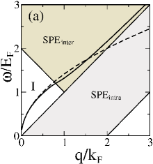
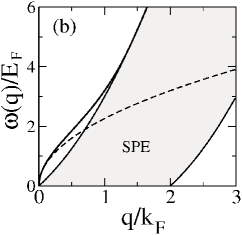
Figure 1: (a) Plasmon mode dispersion in 2D graphene (solid thick line) calculated within RPA. The dashed line indicates the local long wavelength plasmon dispersion. Thin solid lines represent the boundaries of the single particle excitation (SPE) Landau damping regime for intra- and inter-band electron-hole excitations. (b) The plasmon dispersion and SPE for a normal 2D system with a quadratic energy dispersion.

In Fig. 1 we show the calculated plasmon dispersion within RPA (solid line) compared with the classical local plasmon (dashed line). We use the following parameters: $\kappa=2.5$, $\gamma=6.5$eVÅ, and a density $n=10^{12}$ cm^-2. In fig. 1(b) we show the corresponding 2D regular plasmons with n-GaAs parameters ($n=5\times 10^{11}$ cm^-2). In Fig. 1 we also show the electron-hole continuum or single particle excitation (SPE) region in ($q,\omega$) space, which determines the absorption (Landau damping) of the external field at given frequency and wave vector. The SPE continuum is defined by the non-zero value of the imaginary part of the polarizability function, Im$\Pi(q,\omega)\neq 0$. For a normal 2D system only indirect ($q\neq 0$) transition is possible within the band, and the SPE boundaries are given by $\omega_{1,2}=q^{2}/2m\pm qk_{F}/m$. However, for 2D graphene both intraband and interband transition are possible, and the boundaries are given in Fig. 1(a). The intraband SPE boundaries are $\omega_{1}=\gamma q$ (upper boundary) and $\omega_{2}=0$ for $q<2k_{F}$, $\omega_{2}=\gamma q-2E_{F}$ for $q>2k_{F}$ (lower boundary). The direct transition ($q=0$) is also possible from the valence band to the empty conduction band. Due to the phase-space restriction the interband SPE continuum has a gap at small wave vectors. For $q=0$, the transition is not allowed at $0<\omega<2E_{F}$. If the collective mode lies inside the SPE continuum we expect the mode to be damped. Since the normal 2D plasmon lies, at long wave lengths, above the SPE continuum it never decays to electron-hole pair within RPA. But for graphene the plasmon lies inside the interband SPE continuum decaying into electron-hole pairs. Only in the region I of Fig. 1(a) the plasmon is not damped. The other different feature between a normal 2D plasmon and a graphene plasmon occurs at large wave vectors. The normal 2D plasmon mode enters into the SPE continuum at a critical wave vector, and therefore does not exist at very high wave vectors. All spectral weight of the plasmon mode is transferred to the SPE. But the graphene plasmon does not enter into the intraband SPE and exists for all wave vectors, except for its decay into real interband electron-hole pairs in the SPE_inter regime.

Figure 2: Static polarizability for 2D graphene: $\Pi_{tot}=\Pi^{+}+\Pi^{-}$. Here $\Pi(0)=D(E_{F})=g_{s}g_{v}k_{F}/2\pi\gamma$.

IV static screening

Now we consider the static polarizability $\Pi(q,\omega=0)$. From Eq. (9) we have

$$\tilde{\Pi}^{+}(q)=\left\{\begin{matrix}1-\frac{\pi q}{8k_{F}},&q\leq 2k_{F}\cr 1-\frac{1}{2}\sqrt{1-\frac{4k_{F}^{2}}{q^{2}}}-\frac{q}{4k_{F}}\sin^{-1}\frac{2k_{F}}{q},&q>2k_{F}\cr\end{matrix}\right.$$ (22)

and from Eq. (16) we have

$$\tilde{\Pi}^{-}(q)={\pi q}/{8k_{F}}.$$ (23)

Thus, the total static polarizability becomes a constant at $q\leq 2k_{F}$ as in a normal 2D systems, i.e. $\Pi(q)=\Pi^{+}(q)+\Pi^{-}(q)=D(E_{F})$ for $q\leq 2k_{F}$. In Fig. 2 we show the calculated static polarizability as a function of wave vector. For a normal 2D system the screening wave vector, $q_{s}=q_{TF}=g_{s}g_{v}me^{2}/\kappa$, is independent of electron concentration, but for 2D graphene the screening wave vector is given by $q_{s}=g_{s}g_{v}e^{2}k_{F}/\kappa\gamma$ which is proportional to the square root of the density, $n^{1/2}$. In the large momentum transfer regime, $q>2k_{F}$, the static screening increases linearly with $q$ due to the interband transition. This is a very different behavior from a normal 2D system where the static polarizability falls off rapidly for $q>2k_{F}$ with a cusp at $q=2k_{F}$ rmp . The linear increase of the static polarizability with $q$ gives rise to an enhancement of the effective dielectric constant $\kappa^{*}(q\rightarrow\infty)=\kappa(1+g_{s}g_{v}\pi r_{s}/8)$ in graphene. Note that in a normal 2D system $\kappa^{*}\rightarrow\kappa$ as $q\rightarrow\infty$. Thus, the effective interaction in 2D graphene decreases at short wave lengths due to polarization effects. This large wave vector screening behavior is typical of an insulator. Thus, 2D graphene screening is a combination of “metallic” screening (due to $\Pi^{+}$) and “insulating” screening (due to $\Pi^{-}$), leading to overall rather strange screening properties, all of which can be traced back to the zero-gap chiral relativistic nature of graphene.

In may be worthwhile to ask whether the intrinsic graphene contribution, arising strictly from the interband transitions due to the filled valence band (i.e. the $\Pi^{-}$ term in our graphene polarizability), can be absorbed in the effective background lattice dielectric constant $\kappa$ just as one does in a regular semiconductor ($\kappa_{Si}=11.5$; $\kappa_{GaAs}=12.9$) or insulator ($\kappa_{SiO_{2}}=3.9$) in discussing free carrier screening by doping or gating indeed free carriers in conduction (electrons) or valence (holes) bands. In particular, only intraband free carrier screening is explicitly considered in the usual 2D screening function Lindhard2 ; rmp extensively used stern ; hwang in the quantitative analysis of quantum transport in 2D semiconductor devices such as Si MOSFETs, GaAs modulation-doped high-mobility transistors (HEMTs), and undoped gated GaAs heterostructures (HIGFETs). The interband transition induced screening in the semiconductor based 2D structures is included in the theory simply by appropriately modifying the effective background lattice dielectric constant from the usual vacuum value of unity to a value around ten.

To see whether the effect of the interband $\Pi^{-}$ polarizability can be ‘trivially’ absorbed in a background lattice dielectric constant we rewrite a 2D graphene dielectric function $\epsilon(q)=1+v_{c}(q)\Pi(q)$ to obtain:

$$\epsilon(q)=1+\frac{2\pi e^{2}}{\kappa q}\left[\Pi^{-}(q)+\Pi^{+}(q)\right].$$ (24)

Using Eq. (23), $\Pi^{-}(q)=D(E_{F}){\pi q}/{8k_{F}}$, we get $v_{c}(q)\Pi^{-}(q)=\frac{g_{s}g_{v}\pi}{8}\frac{e^{2}}{\kappa\gamma}=\frac{g_{s}g_{v}\pi}{8}r_{s}$. Thus, we have

$$\epsilon(q)=1+\frac{g_{s}g_{v}\pi}{8}r_{s}+v_{c}(q)\Pi^{+}(q).$$ (25)

Introducing an effective intrinsic background graphene dielectric constant

$$\kappa^{*}=1+g_{s}g_{v}\pi r_{s}/8,$$ (26)

we have

$$\epsilon(q)=\kappa^{*}\left[1+\frac{2\pi e^{2}}{\kappa\kappa^{*}q}\Pi^{+}(q)\right].$$ (27)

Writing an effective free carrier 2D graphene dielectric function

$$\epsilon^{+}(q)\equiv 1+v_{c}^{+}(q)\Pi^{+}(q),$$ (28)

where $v_{c}^{+}(q)=2\pi e^{2}/\kappa\kappa^{*}q$, we have

$$\epsilon(q)\equiv\kappa^{*}\epsilon^{+}(q).$$ (29)

Eq. (29) shows that the intrinsic screening contribution arising from the interband $\Pi^{-}$ term can be completely subsumed by introducing an effective graphene background lattice dielectric constant $\kappa^{*}=1+g_{s}g_{v}\pi r_{s}/8$, and by making the replacement $\kappa\rightarrow\kappa\kappa^{*}$ throughout. Introducing the effective dielectric constant $\kappa^{*}$ allows one to use only the free carrier screening function

$$\epsilon^{+}(q)=1+\frac{2\pi e^{2}}{\kappa\kappa^{*}q}\Pi^{+}(q),$$ (30)

for describing free carrier screening properties of 2D graphene. We note that $\kappa$ itself here is the background lattice dielectric constant arising from the insulating substrate (i.e. SiO₂ in most situations) with $\kappa=(1+\kappa_{SiO_{2}})/2\approx 2.5$, and $\kappa^{*}=1+g_{s}g_{v}\pi r_{s}/8\approx 2.3$ with $r_{s}=e^{2}/\kappa\hbar\gamma\approx 0.7$ for graphene on SiO₂ substrate. Thus, the substitution $\kappa\rightarrow\kappa\kappa^{*}$ arising from the interband contributions enhances the effective background graphene dielectric constant to $\kappa\kappa^{*}\approx 6$ — this approximate factor of 2 increase in the background dielectric constant arising from interband contributions further suppress Coulomb interaction effects in extrinsic graphene.

The large $q$ behavior of graphene dielectric screening, $\epsilon(q\rightarrow\infty)\rightarrow\kappa^{*}=1+g_{s}g_{v}\pi r_{s}/8$, again demonstrates that the short-wavelength screened Coulomb potential in 2D graphene goes as $2\pi e^{2}/\kappa\kappa^{*}q$, with an enhanced background effective dielectric constant $\kappa\kappa^{*}$ where $\kappa$ is the effective background dielectric constant arising from the substrate and $\kappa^{*}$ arising from graphene interband polarizability $\Pi^{-}$ as discussed above. This implies that a suspended 2D graphene film, without any substrate (i.e. $\kappa=1$), would have an effective background lattice dielectric constant of $\kappa^{*}=1+g_{s}g_{v}\pi r_{s}/8$ with $r_{s}=e^{2}/\hbar\gamma$ (since $\kappa=1$). Putting in $g_{s}g_{v}=4$, we get $\kappa^{*}\approx 4$. Thus the background static lattice dielectric constant of intrinsic graphene, due to interband transitions, is around 4.

If the $T=0$ transport properties of graphene are dominated by charged impurity scattering as is thought to be the case hwang_g then the long-wavelength Thomas-Fermi screening becomes an important input for calculating the screened charged impurity potential: $\epsilon_{TF}(q)\equiv\epsilon_{RPA}(q\rightarrow 0)$ becomes

$$\epsilon_{TF}(q)=1+q_{TF}/q,$$ (31)

where $q_{TF}\equiv q_{s}=g_{s}g_{v}e^{2}k_{F}/\kappa\gamma$. Note that one can equivalently define a long wavelength effective TF screening function $\epsilon_{TF}^{+}(q)$ where interband screening effects are absorbed in an effective background dielectric constant $\kappa^{*}$;

$$\epsilon^{+}_{TF}(q)=1+q_{TF}^{*}/q,$$ (32)

where $q_{TF}^{*}=q_{TF}/\kappa^{*}$. As discussed above, the identity, $\epsilon(q)\equiv\kappa^{*}\epsilon^{+}(q)$, guarantees the equivalence between Eqs. (31) and (32) for long wavelength graphene screening. We note also that the $q=0$ screening wavevector $q_{TF}$ is simply proportional to the graphene density of states at the Fermi level at $T=0$.

Although the two screening descriptions, based on $\epsilon(q)$ with the background dielectric constant being just $\kappa$ and on $\epsilon^{+}(q)$ with the background dielectric constant being $\kappa\kappa^{*}$, are precisely equivalent for $T=0$ static screening properties, the two descriptions are not inequivalent at finite temperatures. Therefore, it is more appropriate to use the full dielectric function $\epsilon(q)$ in theoretical work on 2D graphene.

V conclusion

In conclusion, we have theoretically obtained analytic expressions for doped (i.e. $E_{F}\neq 0$) 2D extrinsic graphene polarizability, dielectric function, plasmon dispersion, and static screening properties, finding a number of intriguing qualitative differences with the corresponding normal (and extensively studied) 2D electron systems. The differences, with interesting observable consequences, can all be understood as arising from the zero-band gap intrinsic nature of undoped graphene with chiral linear relativistic bare carrier energy band dispersion. Some of our qualitatively new predictions, such as the $n^{1/4}$ dependence of the long-wave length graphene plasma frequency in contrast to the well-known $n^{1/2}$ behavior of classical and normal 2D plasmons, should be easily verifiable experimentally using the standard experimental techniques of infra-red absorption Tsui and/or inelastic light scattering Olego spectroscopies. Similarly, our prediction of the peculiar nature of the graphene plasmon damping (i.e. no Landau damping due to intraband electron-hole pairs, but finite Landau damping due to interband electron-hole pairs) should be easily verifiable. Our predicted different screening behavior in graphene at large wave vector should have consequences for transport properties. Our RPA theory should be an excellent qualitative approximation for 2D graphene properties at all carrier densities (as long as the system remains a homogeneous 2D carrier system, which may not be true for $n\lesssim 10^{12}cm^{-2}$) since the effective $r_{s}$-parameter for graphene is a constant ($<1$), making RPA quantitatively accurate in graphene. Finally, we point out that the effective Fermi temperature, $T_{F}=E_{F}/k_{B}$, being very high ($\sim 1300K$ for $n\sim 10^{12}$ cm^-2) in graphene, our $T=0$ theory should apply all the way to room temperatures. We note that the long wavelength dielectric function for bulk graphite was earlier considered within an approximation scheme in ref. Shung, , and the zero frequency limit was recently considered in ref. Ando, .

Before concluding, we point out that some aspects of graphene collective modes and linear response have been discussed in the recent literature. In particular, the intrinsic situation without any free carriers has been considered in khve whereas our emphasis in this work has been extrinsic graphene with free carriers (electrons/holes in conduction/valence band) induced by external gating or doping. There has been a recent purely numerical study wang of graphene collective mode spectra in the presence of spin-orbit coupling.

Note added After submitting the present paper, we became aware of related work wunsch .

This work is supported by the US-ONR, the LPS, and the Microsoft corporation.

References

- (1) K.S. Novoselov, A.K. Geim, S.V. Morozov, D. Jiang, M.I. Katsnelson, I.V. Grigorieva, S.V. Dubonos, and A.A. Firsov, Nature 438, 197 (2005); Science 306, 666 (2004).
- (2) Y. Zhang, Y. W. Tan, H. L. Stormer, and P. Kim, Nature 438, 201 (2005).
- (3) T. Ando, A. B. Fowler, and F. Stern, Rev. Mod. Phys. 54, 437 (1982).
- (4) G.D. Mahan, Many Particle Physics, (Plenum, New York, 1993)
- (5) Frank Stern, Phys. Rev. Lett. 18, 546 (1967).
- (6) J. Gonzalez, F. Guinea, and M. A. H. Vozmediano, Nucl. Phys. B 424, 595 (1994).
- (7) D. V. Khveshchenko, Phys. Rev. B 74, 161402(R) (2006); O. Vafek, Phys. Rev. Lett. 97, 266406 (2006).
- (8) X.F. Wang and T. Chakraborty, Phys. Rev. B 75, 033408 (2007); Phys. Rev. B 75, 041404(R) (2007).
- (9) S. Das Sarma and A. Madhukar, Phys. Rev. B23, 805 (1981).
- (10) S. Das Sarma and E. H. Hwang, Phys. Rev. Lett. 81, 4216 (1998).
- (11) S. J. Allen, Jr., D. C. Tsui, and R. A. Logan, Phys. Rev. Lett. 38, 980 (1977).
- (12) D. Olego. A. Pinczuk, A. C. Grossard, and W. Wiegmann, Phys. Rev. B25, 7867 (1982).
- (13) F. Stern, Phys. Rev. Lett. 44, 1469 (1980)
- (14) S. Das Sarma and E. H. Hwang, Phys. Rev. Lett. 83, 164 (1999); Solid State Commun. 135, 579 (2005); Phys. Rev. B 69, 195305 (2004).
- (15) E. H. Hwang, S. Adam, and S. Das Sarma, cond-mat/0610157.
- (16) K. W. K Shung, Phys. Rev. B34 979 (1986).
- (17) T. Ando, J. Phys. Soc. Jpn. 75, 074716 (2006).
- (18) B. Wunsch, T. Stauber, F. Sols, and F. Guinea, New. J.Phys. 8, 318 (2006).