Semiclassical Approach to Chaotic Quantum Transport

Abstract

We describe a semiclassical method to calculate universal transport properties of chaotic cavities. While the energy-averaged conductance turns out governed by pairs of entrance-to-exit trajectories, the conductance variance, shot noise and other related quantities require trajectory quadruplets; simple diagrammatic rules allow to find the contributions of these pairs and quadruplets. Both pure symmetry classes and the crossover due to an external magnetic field are considered.

I INTRODUCTION

Mesoscopic cavities show universal transport properties – such as conductance, conductance fluctuations, or shot noise – provided the classical dynamics inside the cavity is fully chaotic. Here chaos may be due to either implanted impurities or bumpy boundaries. A phenomenological description of these universal features is available through random-matrix theory (RMT) by averaging over ensembles of systems (whose Hamiltonians are represented by matrices) Beenakker . For systems with impurities, one can alternatively average over different disorder potentials. However, experiments show that even individual cavities show universal behavior faithful to these averages.

In the present paper we want to show why this is the case. To do so we propose a semiclassical explanation of universal transport through individual chaotic cavities, based on the interfering contributions of close classical trajectories. This approach generalizes earlier work in RS ; Schanz ; EssenCond ; EssenShot and is inspired by recent progress for universal spectral statistics Berry ; Argaman ; SR ; EssenFF . Our semiclassical procedure often turns out to be technically easier than RMT; transport properties are evaluated through very simple diagrammatic rules.

We consider a two-dimensional cavity accommodating chaotic classical motion. Two (or more) straight leads are attached to the cavity and carry currents. We shall mostly consider electronic currents, but most of the following ideas apply to transport of light or sound as well, minor modifications apart.

The leads support wave modes (“channels”) ${\rm e}^{{{\rm i}}kx_{i}\cos\theta_{i}}\sin(ky_{i}\sin|\theta_{i}|)$; the subscripts $i=1,2$ refer to the ingoing and outgoing lead, respectively, $x_{i}$ and $y_{i}$ with $0<y_{i}<w_{i}$ are coordinates along and transversal to the lead. Here, $w_{i}$ is the width of the lead, $k$ the wave number, and $\theta_{i}$ the angle enclosed between the wave vector and the direction of the lead. Dirichlet boundary conditions inside the lead impose the restriction $kw_{i}\sin|\theta_{i}|=a_{i}\pi$ with the channel index $a_{i}$ running from 1 to $N_{i}$, the largest integer below $\frac{kw_{i}}{\pi}$. Classically, the $a_{i}$-th channel can be associated with trajectories inside the lead that enclose an angle $\theta_{i}$ with the lead direction, regardless of their location in configuration space. The sign of the enclosed angle changes after each reflection at the boundaries of the cavity, and angles of both signs are associated to the same channel.

We shall determine, e.g., the mean and the variance of the conductance as power series in the inverse of the number of channels $N=N_{1}+N_{2}$. In contrast to much of the previous literature, we will go to all orders in $\frac{1}{N}$. We shall be interested both in dynamics with time reversal invariance (“orthogonal case”) and without that symmetry (“unitary case”). For electronic motion time reversal invariance may be broken by an external magnetic field. For that latter case, we shall also interpolate between both pure symmetry classes by account for a weak magnetic field producing magnetic actions of the order of $\hbar$.

We will always work in the semiclassical limit, and thus require the linear dimension $L$ of the cavity to be large compared to the (Fermi) wavelength $\lambda$. When taking the limit $\frac{\lambda}{L}\to 0$, the number of channels $N\propto\frac{w}{\lambda}$ ($w\sim w_{1}\sim w_{2}$) will be increased only slowly. The width of the openings thus becomes small compared to $L$. For this particular semiclassical limit, the dwell time of trajectories inside the cavity, $T_{D}\propto\frac{L}{w}$ grows faster than the so-called Ehrenfest time $T_{E}\propto\ln\frac{L}{\lambda}\propto\ln\hbar$. Interesting effects arising for $T_{E}/T_{D}$ of order unity Brouwer ; Whitney ; EhrenfestRMT are thus discarded.

Following Landauer and Büttiker Landauer ; Buettiker , we view transport as scattering between leads and deal with amplitudes $t_{a_{1}a_{2}}$ for transitions between channels $a_{1}$ and $a_{2}$. These amplitudes form an $N_{1}\times N_{2}$ matrix $t=\{t_{a_{1}a_{2}}\}$. Each $t_{a_{1}a_{2}}$ can be approximated semiclassically, by the van Vleck approximation for the propagator, as a sum over trajectories connecting the channels $a_{1}$ and $a_{2}$ Richter ,

$$t_{a_{1}a_{2}}\sim\frac{1}{\sqrt{T_{H}}}\sum_{\alpha:a_{1}\to a_{2}}A_{\alpha}{\rm e}^{{{\rm i}}S_{\alpha}/\hbar}\,.$$ (1)

The channels exactly determine the absolute values of the initial and final angles of incidence $\theta_{1},\theta_{2}$ of the contributing trajectories; again both positive and negative angles are possible. In (1), $T_{H}$ denotes the so-called Heisenberg time, i.e., the quantum time scale $2\pi\hbar\overline{\rho}$ associated to the mean level density $\overline{\rho}$. The Heisenberg time diverges in the semiclassical limit like $T_{H}=2\pi\hbar\overline{\rho}\sim\frac{\Omega}{(2\pi\hbar)^{f-1}}$ with $\Omega$ the volume of the energy shell and $f$ the number of degrees of freedom; we shall mostly consider $f=2$. The “stability amplitude” $A_{\alpha}$ (which includes the so-called Maslov index) can be found in Richter’s review Richter . Finally, the phase in (1) depends on the classical action $S_{\alpha}=\int_{\alpha}{\bf p}\cdot d{\bf q}$.

Within the framework just delineated, we will evaluate, for individual fully chaotic cavities,

• the mean conductance $\big{\langle}{\rm tr}(tt^{\dagger})\big{\rangle}$ (Actually, the conductance is given by $\frac{e^{2}}{\pi\hbar}\big{\langle}{\rm tr}(tt^{\dagger})\big{\rangle}$, taking into account two possible spin orientations; we prefer to express the result in units of $\frac{e^{2}}{\pi\hbar}$),

• the conductance variance $\big{\langle}({\rm tr}\;tt^{\dagger})^{2}\big{\rangle}-\big{\langle}{\rm tr}(tt^{\dagger})\big{\rangle}^{2}$,

• the mean shot noise power $\big{\langle}{\rm tr}(tt^{\dagger}-tt^{\dagger}tt^{\dagger})\big{\rangle}$, in units of $\frac{2e^{3}|V|}{\pi\hbar}$,

• for a cavity with three leads, correlations between the currents flowing from lead 1 to lead 2 and from lead 1 to lead 3 depending on the corresponding transition matrices $t^{(1\to 2)},t^{(1\to 3)}$ as $\big{\langle}{\rm tr}(t^{(1\to 2)}{t^{(1\to 2)}}^{\dagger}t^{(1\to 3)}{t^{(1\to 3)}}^{\dagger})\big{\rangle}$,

• the conductance covariance at two different energies which characterizes the so-called Ericson fluctuations.

Here the angular brackets signify an average over an energy interval sufficient to smooth out the fluctuations of the respective physical property. We will see that after such an averaging each of these quantities takes a universal form in agreement with random-matrix theory, without any need for an ensemble average. To show this, we shall express the transition amplitudes as sums over trajectories as in (1). The above observables then turn into averaged sums over pairs or quadruplets of trajectories, which will be evaluated according to simple and universal diagrammatic rules. We shall first derive and exploit these rules for the orthogonal and unitary cases and then generalize to the interpolating case (weak magnetic field).

Due to the unitarity of the time evolution, we could equivalently express transport properties through reflection amplitudes and trajectories starting and ending at the same lead. For the average conductance we have checked explicitly that the same result is obtained, meaning that our approach preserves unitarity.

II Mean conductance

We first consider the mean conductance and propose to show that individual chaotic systems are faithful to the random-matrix prediction Beenakker ; Conductance

$$\big{\langle}G(E)\big{\rangle}=\big{\langle}{\rm tr}(tt^{\dagger})\big{\rangle}=\begin{cases}\frac{N_{1}N_{2}}{N}&\text{unitary case}\\ \frac{N_{1}N_{2}}{N+1}&\text{orthogonal case}\,.\end{cases}$$ (2)

In the semiclassical approximation (1), the average conductance becomes a double sum over trajectories $\alpha,\beta$ connecting the same channels $a_{1}$ and $a_{2}$,

$$\big{\langle}{\rm tr}(tt^{\dagger})\big{\rangle}=\left\langle\sum_{a_{1},a_{2}}t_{a_{1}a_{2}}t_{a_{1}a_{2}}^{*}\right\rangle=\frac{1}{T_{H}}\left\langle\sum_{a_{1},a_{2}}\sum_{\alpha,\beta:a_{1}\to a_{2}}A_{\alpha}A_{\beta}^{*}{\rm e}^{{{\rm i}}(S_{\alpha}-S_{\beta})/\hbar}\right\rangle\,.$$ (3)

Due to the phase factor ${\rm e}^{{{\rm i}}(S_{\alpha}-S_{\beta})/\hbar}$, the contributions of most trajectory pairs oscillate rapidly in the limit $\hbar\to 0$, and vanish after averaging over the energy. Systematic contributions can only arise from pairs with action differences $\Delta S=S_{\alpha}-S_{\beta}$ of the order of $\hbar$.

II.1 Diagonal contribution

The simplest such pairs involve identical trajectories $\alpha=\beta$, with a vanishing action difference Berry ; Baranger . These “diagonal” pairs contribute

$$\big{\langle}{\rm tr}(tt^{\dagger})\big{\rangle}\big{|}_{\rm diag}=\frac{1}{T_{H}}\left\langle\sum_{a_{1},a_{2}}\sum_{\alpha:a_{1}\to a_{2}}|A_{\alpha}|^{2}\right\rangle\,.$$ (4)

The foregoing single-trajectory sum may be evaluated using the following rule established by Richter and Sieber RS : Summation over trajectories connecting fixed channels is equivalent to integration over the dwell time $T$ as

$$\sum_{\alpha:a_{1}\to a_{2}}|A_{\alpha}|^{2}=\int_{0}^{\infty}dT{\rm e}^{-\frac{N}{T_{H}}T}=\frac{T_{H}}{N}\,.$$ (5)

Here, the integrand ${\rm e}^{-\frac{N}{T_{H}}T}$ can be understood as the survival probability, i.e., the probability for the trajectory to remain inside the cavity up to the time $T$. The factor $\frac{N}{T_{H}}=\frac{2p(w_{1}+w_{2})}{\Omega}$ is the classical escape rate. Due to $\Omega\propto L^{2}$, that rate is proportional to $\frac{w}{L}$ if $p$ is scaled according to $p\propto L$; inversion yields the typical dwell time $T_{D}=\frac{T_{H}}{N}\propto\frac{L}{w}$ mentioned in the introduction.

Finally summing over all $N_{1}$ possible choices for $a_{1}$ and over the $N_{2}$ possibilities for $a_{2}$, one finds Baranger ; RS

$$\big{\langle}{\rm tr}(tt^{\dagger})\big{\rangle}\big{|}_{\rm diag}=\frac{N_{1}N_{2}}{N}\,.$$ (6)

Eq. (6) reproduces the RMT result for the unitary case, and gives the leading term in the orthogonal case.

II.2 Richter/Sieber pairs

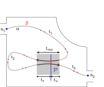
Figure 1: Scheme of a Richter/Sieber pair. The trajectories $\alpha$ (full line) and $\beta$ (dashed line) connect the same channels $a_{1}$ and $a_{2}$, and differ only inside a 2-encounter (in the box). A Poincaré section ${\cal P}$ intersects the encounter stretches at the points ${\bf x}_{{\cal P}1}$ and ${\bf x}_{{\cal P}2}$ in phase space whose configuration-space location is highlighted by two dots. ${\cal P}$ divides the encounter in two parts with durations $t_{s}\sim\frac{1}{\lambda}\ln\frac{c}{|s|}$ and $t_{u}\sim\frac{1}{\lambda}\ln\frac{c}{|u|}$. The relevant trajectories are in reality much longer than depicted here; in the absence of a potential they consist of a huge number of straight segments reflected at the boundary.

For the orthogonal case, Richter and Sieber attributed the next-to-leading order to another family of trajectory pairs. In the following, we shall describe these pairs in a language adapted to an extension to higher orders in $\frac{1}{N}$. In each Richter/Sieber pair (see Fig. 1), the trajectory $\alpha$ contains a “2-encounter” wherein two stretches are almost mutually time-reversed; in configuration space it looks like either a small-angle self-crossing or a narrow avoided crossing. We demand that these two stretches come sufficiently close such that their motion is mutually linearizable. Along $\alpha$, the two stretches are separated from each other and from the leads by three “links” . The partner trajectory $\beta$ is distinguished from $\alpha$ only by differently connecting these links inside the 2-encounter. Along the links, however, $\beta$ is practically indistinguishable from $\alpha$; in particular, the entrance and exit angles of $\alpha$ and $\beta$ (defined by the in- and out-channels) coincide . The initial and final links are traversed in the same sense of motion by $\alpha$ and $\beta$, while for the middle link the velocities are opposite. Obviously, such Richter/Sieber pairs $\alpha,\beta$ can exist only in time-reversal invariant systems. The two trajectories in a Richter/Sieber pair indeed have nearly the same action, with the action difference originating mostly from the encounter region.

We stress that inside a Richter/Sieber pair, the encounter stretches and the leads must be separated by links of positive durations $t_{1},t_{2},t_{3}>0$. For the “inner” loop with duration $t_{2}$ the reasons were worked out in previous publications dealing with periodic orbits (Mueller ; HigherDim , and EssenFF ; MuellerThesis for more complicated encounters): Essentially, $\beta$ is obtained from $\alpha$ by switching connections between four points where the encounter stretches begin and end; to have four such points the stretches must be separated by a non-vanishing link. The fact that the duration of the initial and final links is non-negative (the encounter does not “stick out” through any of the openings) is trivial in the case of the Richter/Sieber pair: Since the encounter stretches are almost antiparallel a trajectory with an encounter “sticking out” would enter and exits the cavity through the same opening and thus be irrelevant for the conductance.

Encounters have an important effect on the survival probability EssenCond . The trajectory $\alpha$ is exposed to the “danger” of getting lost from the cavity only during the three links and on the first stretch of the encounter. If the first stretch remains inside the cavity, the second stretch, being close to the first one (up to time reversal) must remain inside as well. If we denote the duration of one encounter stretch by $t_{\rm enc}$, the total “exposure time” is thus given by $T_{\rm exp}=t_{1}+t_{2}+t_{3}+t_{\rm enc}$; it is shorter than the dwell time $T$ which includes a second summand $t_{\rm enc}$ representing the second encounter stretch. Consequently, the survival probability ${\rm e}^{-\frac{N}{T_{H}}T_{\rm exp}}$ exceeds the naive estimate ${\rm e}^{-\frac{N}{T_{H}}T}$. In brief, encounters hinder the loss of a trajectory to the leads.

To describe the phase-space geometry of a 2-encounter, we consider a Poincaré section ${\cal P}$ orthogonal to the first encounter stretch in an arbitrary phase-space point ${\bf x}_{{\cal P}1}$. This section must also intersect the second stretch in a phase-space point ${\bf x}_{{\cal P}2}$ almost time-reversed with respect to ${\bf x}_{{\cal P}1}$. In Fig. 1 the configuration-space locations of ${\bf x}_{{\cal P}1}$ and ${\bf x}_{{\cal P}2}$ are highlighted by two dots. For a hyperbolic, quasi two-dimensional system, the small phase space separation between the time-reversed ${\cal T}{\bf x}_{{\cal P}2}$ of ${\bf x}_{{\cal P}2}$ and ${\bf x}_{{\cal P}1}$ can be decomposed as Gaspard ; Spehner ; Turek

$${\cal T}{\bf x}_{{\cal P}2}-{\bf x}_{{\cal P}1}=s{\bf e}^{s}({\bf x}_{{\cal P}1})+u{\bf e}^{u}({\bf x}_{{\cal P}1})\,,$$ (7)

where ${\bf e}^{s}({\bf x}_{{\cal P}1})$ and ${\bf e}^{u}({\bf x}_{{\cal P}1})$ are the so-called stable and unstable directions at ${\bf x}_{{\cal P}1}$. If ${\cal P}$ moves along the trajectory, following the time evolution of ${\bf x}_{{\cal P}1}$, the unstable component $u$ will grow exponentially while the stable component $s$ shrinks exponentially. For times large compared with the ballistic time ($L/v$ with $v$ the velocity) the rate of growth (or shrinking) is given by the Lyapunov exponent $\lambda$ (not to be confused with the wavelength also denoted by $\lambda$),

$$u(t) \sim u(0){\rm e}^{\lambda t}$$

$$s(t) \sim s(0){\rm e}^{-\lambda t}\,.$$ (8)

By our definition of a 2-encounter, the stable and unstable components are confined to ranges $-c<s<c$, $-c<u<c$, with $c$ a small phase-space separation. The exact value of $c$ will be irrelevant, except that the transverse size of the encounter in configuration space, $\sim c/\sqrt{m\lambda}$ with $m$ the mass, must be small compared with the opening diameters. It should also be small enough to allow mutual linearization of motion along the encounter stretches. As a consequence, the time between ${\cal P}$ and the end of the encounter is $t_{u}\sim\frac{1}{\lambda}\ln\frac{c}{|u|}$, i.e., the time the unstable component needs to grow from $u$ to $\pm c$. Likewise the time between the beginning of the encounter and ${\cal P}$ reads $t_{s}\sim\frac{1}{\lambda}\ln\frac{c}{|s|}$. Both times sum up to the encounter duration

$$t_{\rm enc}=t_{u}+t_{s}\sim\frac{1}{\lambda}\ln\frac{c^{2}}{|su|}\,.$$ (9)

A glance at Fig. 1 shows that the times $t_{{\cal P}1},t_{{\cal P}2}$ of the piercing points ${\bf x}_{{\cal P}1}$, ${\bf x}_{{\cal P}2}$ (measured from the beginning of the trajectory) are now given by

$$t_{{\cal P}1}=t_{1}+t_{u},\quad t_{{\cal P}2}=t_{1}+t_{\rm enc}+t_{2}+t_{s}\,.$$ (10)

Finally, the stable and unstable coordinates determine the action difference as Spehner ; Turek (see also Mueller ; EssenFF )

$$\Delta S=su\,.$$ (11)

The encounters relevant for the transport phenomena have action differences of order $\hbar$ and thus durations $t_{\rm enc}\sim\frac{1}{\lambda}\ln\frac{c^{2}}{|\Delta S|}$ of the order of the Ehrenfest time $T_{E}=\frac{1}{\lambda}\ln\frac{c^{2}}{\hbar}$.

With this input, we can determine the average number of 2-encounters inside trajectories $\alpha$ of a given dwell time $T$. In ergodic systems, the probability for a trajectory to pierce through a fixed Poincaré section ${\cal P}$ in a time interval $(t_{{\cal P}2},t_{{\cal P}2}+dt_{{\cal P}2})$ with stable and unstable separations from ${\bf x}_{{\cal P}1}$ inside $(s,s+ds)\times(u,u+du)$ is uniform, and given by the Liouville measure $\frac{1}{\Omega}dt_{{\cal P}2}dsdu$. To count all 2-encounters inside $\alpha$, we have to integrate this density over $t_{{\cal P}2}$ (to get all piercings ${\bf x}_{{\cal P}2}$ through a given ${\cal P}$) and over $t_{{\cal P}1}$ (to get all possible ${\bf x}_{{\cal P}1}$ and thus all possible sections ${\cal P}$). When integrating over $t_{{\cal P}1}$, we weigh the contribution of each encounter with the corresponding duration $t_{\rm enc}$, since the section ${\cal P}$ may be placed at any point within the encounter; therefore we must subsequently divide by $t_{\rm enc}$. The integration over the piercing times $t_{{\cal P}1}$, $t_{{\cal P}2}$ may be replaced by integration over the link durations $t_{1},t_{2}$, which as we stressed, must be positive; in addition $t_{3}=T-t_{1}-t_{2}-2t_{\rm enc}$ must also be positive. Altogether, we obtain the following density of stable and unstable coordinates,

$$w(s,u)=\int_{t_{1},t_{2}>0\atop t_{1}+t_{2}<T-2t_{\rm enc}}dt_{1}dt_{2}\;\frac{1}{\Omega\,t_{\rm enc}(s,u)}\,.$$ (12)

This density is normalized such that integration over all $s,u$ belonging to a given interval of $\Delta S=su$ yields the number of 2-encounters of $\alpha$ giving rise to action differences within that interval.

To find what Richter/Sieber pairs contribute to the conductance (3), we replace the sum over $\beta$ by a sum over 2-encounters inside $\alpha$ or, equivalently, an integral over $w(s,u)$. The additional approximation $A_{\beta}\approx A_{\alpha}$ yields

$$\big{\langle}{\rm tr}(tt^{\dagger})\big{\rangle}\big{|}_{\rm RS}=\frac{1}{T_{H}}\left\langle\sum_{a_{1},a_{2}}\int dsdu\sum_{\alpha:a_{1}\to a_{2}}|A_{\alpha}|^{2}w(s,u){\rm e}^{{{\rm i}}su/\hbar}\right\rangle\,.$$ (13)

Next, we employ the Richter/Sieber rule to do the sum over $\alpha$ by integrating over the dwell time $T$, with the integrand involving the (modified) survival probability ${\rm e}^{-\frac{N}{T_{H}}T_{\rm exp}}={\rm e}^{-\frac{N}{T_{H}}(t_{1}+t_{2}+t_{3}+t_{\rm enc})}$. The integral over $T$ may be transformed into an integral over the duration of the final link. Moreover, summation over all channels $a_{1}=1\ldots N_{1}$, $a_{2}=1\ldots N_{2}$ yields a factor $N_{1}N_{2}$. We are thus led to

$$\big{\langle}{\rm tr}(tt^{\dagger})\big{\rangle}\big{|}_{\rm RS}=\frac{N_{1}N_{2}}{T_{H}}\left\langle\int_{0}^{\infty}dt_{1}dt_{2}dt_{3}\int dsdu\frac{1}{\Omega\,t_{\rm enc}(s,u)}{\rm e}^{-\frac{N}{T_{H}}(t_{1}+t_{2}+t_{3}+t_{\rm enc}(s,u))}{\rm e}^{{{\rm i}}su/\hbar}\right\rangle\,.$$ (14)

This integral factors into three independent integrals over the link durations,

$$\int_{0}^{\infty}dt_{i}{\rm e}^{-\frac{N}{T_{H}}t_{i}}=\frac{T_{H}}{N}\,,$$ (15)

and an integral over the stable and unstable separations within the encounter,

$$I=\left\langle\int dsdu\frac{1}{\Omega\,t_{\rm enc}(s,u)}{\rm e}^{-\frac{N}{T_{H}}t_{\rm enc}(s,u)}{\rm e}^{{{\rm i}}su/\hbar}\right\rangle\,.$$ (16)

The encounter integral $I$ can be evaluated if we expand the exponential as ${\rm e}^{-\frac{N}{T_{H}}t_{\rm enc}(s,u)}=1-\frac{N}{T_{H}}t_{\rm enc}(s,u)+\ldots$. As shown in EssenFF , the constant term yields $\big{\langle}dsdu\frac{1}{\Omega\,t_{\rm enc}(s,u)}{\rm e}^{{{\rm i}}su/\hbar}\big{\rangle}=\big{\langle}\frac{2\lambda\hbar}{\Omega}\sin\frac{c^{2}}{\hbar}\big{\rangle}$ which oscillates rapidly as $\hbar\to 0$ and therefore vanishes after averaging. In the semiclassical limit, the value of $I$ is solely determined by the linear term for which the denominator $t_{\rm enc}(s,u)$ cancels out,

$$I=-\frac{N}{\Omega T_{H}}\left\langle\int dsdu{\rm e}^{{{\rm i}}su/\hbar}\right\rangle=-\frac{N}{T_{H}^{2}}\,,$$ (17)

where we use$\int dsdu{\rm e}^{{{\rm i}}su/\hbar}\to 2\pi\hbar$ and $T_{H}=\frac{\Omega}{2\pi\hbar}$; all further terms vanish compared to the linear one like $\frac{Nt_{\rm enc}}{T_{H}}\sim\frac{T_{E}}{T_{D}}$ and may thus be neglected, given our previous definition of the semiclassical limit. Since all occurrences of $T_{H}$ in Eqs. (14), (15) and (17) mutually cancel, we can formulate the following “diagrammatic rule”: Each link yields a factor $\frac{1}{N}$ and each encounter a factor $-N$. The result still has to be multiplied with the number of channel combinations $N_{1}N_{2}$. Altogether, the contribution of Richter/Sieber pairs to the average conductance is hence determined as

$$\big{\langle}{\rm tr}(tt^{\dagger})\big{\rangle}\big{|}_{\rm RS}=-\frac{N_{1}N_{2}}{N^{2}}\,.$$ (18)

Our present treatment differs from Richter’s and Sieber’s original paper RS in two points: First, one has to exclude encounters which stick out of the opening. (In RS , encounters were described through self-crossings in configuration space, and only that crossing, approximately in the center of the encounter, had to be located inside the cavity.) Second, one must take into account that encounters hinder the escape into the leads. While these two corrections mutually cancel for Richter/Sieber pairs they will presently turn out of crucial importance for higher-order contributions to the mean conductance, as well as for other observables like shot noise.

II.3 Diagrammatic rules for all orders in $\frac{1}{N}$

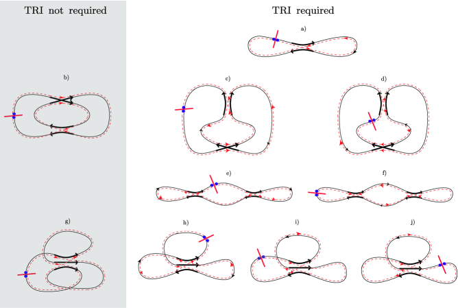
Figure 2: Families of trajectory pairs $(\alpha,\beta)$ differing in one 2-encounter (a), two 2-encounters (b-f) or in one 3-encounter (g-j). In contrast to Fig. 1 the cavity is not depicted, and the initial and final points of the trajectories are joined together (junction symbolized by two dots and intervening bar, $\cdot|\cdot$). One orbit pair may result from joining beginning and end of different trajectory pairs (like cd, ef, and hij). Arrows indicate the directions of motion inside the encounters, and highlight those links which are traversed by $\alpha$ and $\beta$ with opposite sense of motion. Note that all families apart from b) and g) involve almost mutually time-reversed encounter stretches and thus require time-reversal invariance (TRI). Together with the diagonal pairs, the ones shown here reproduce the mean conductance up to order $N_{1}N_{2}/N^{3}$.

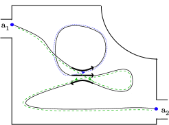
Figure 3: Reconnections inside a 3-encounter leading to one trajectory (dashed) and one periodic orbit (dotted), rather than a single connected partner trajectory.

To proceed to all orders in $\frac{1}{N}$, we must consider pairs of trajectories differing by their connections inside arbitrarily many encounters. Each of these encounters may involve arbitrarily many stretches. We shall speak of an $l$-encounter whenever $l$ stretches of a trajectory come close in phase space. In time-reversal invariant systems we must also allow for encounters whose stretches are almost mutually time-reversed. As a consequence, the resulting conductance will depend on the symmetry class: We shall see all higher-order contributions to mutually cancel in the unitary case but to yield the $1/N$ expansion of the RMT result (2) in the orthogonal case.

A list of examples is displayed in Fig. 2, where for later convenience we did not draw the cavity and formally joined the initial and final points of the trajectories together. These examples illustrate the simplest among infinitely many topologically different families of trajectory pairs.

The individual families are characterized (i) by the numbers $v_{l}$ of $l$-encounters in which the two partners differ. These numbers can be assembled into a “vector”$\vec{v}=(v_{2},v_{3},v_{4},\ldots)$, and determine the overall number of encounters $V(\vec{v})=\sum_{l\geq 2}v_{l}$ and the total number of encounter stretches $L(\vec{v})=\sum_{l\geq 2}lv_{l}$. The number of links exceeds the number of stretches by one and reads $L(\vec{v})+1$. Further characteristics of our families of trajectory pairs are (ii) the order in which the encounters are traversed by the trajectory $\alpha$, (iii) the mutual orientation of the encounter stretches (i.e., $\mathrel{\,\lower 0.6458pt\hbox{\begin{picture}(4.0,3.0)\put(0.0,0.8){\vector(1,0){4.0}}\put(0.0,2.0){\vector(1,0){4.0}}\end{picture}}\,}$ vs. $\mathrel{\,\lower 0.6458pt\hbox{\begin{picture}(4.0,3.0)\put(4.0,0.8){\vector(-1,0){4.0}}\put(0.0,2.0){\vector(1,0){4.0}} \end{picture}}\,}$, or $\mathrel{\,\lower 0.6458pt\hbox{\begin{picture}(4.0,3.0)\put(0.0,0.3){\vector(1,0){4.0}}\put(0.0,1.5){\vector(1,0){4.0}} \put(0.0,2.7){\vector(1,0){4.0}} \end{picture}}\,}$ vs. $\mathrel{\,\lower 0.6458pt\hbox{\begin{picture}(4.0,3.0)\put(4.0,0.3){\vector(-1,0){4.0}}\put(0.0,1.5){\vector(1,0){4.0}} \put(0.0,2.7){\vector(1,0){4.0}} \end{picture}}\,}$), and (iv) the reconnections leading to the partner trajectory $\beta$. We stress that $\beta$ must be a single connected trajectory; reconnections leading to, e.g., one trajectory and one periodic orbit as in Fig. 3 must be excluded.

All families of trajectory pairs contribute to the conductance according to the same rules as do Richter/Sieber pairs: Each link yields a factor $\frac{1}{N}$, each encounter gives a factor $-N$, and we have to multiply with the number of channel combinations $N_{1}N_{2}$. To prove this assertion, we place a Poincaré section ${\cal P}_{\sigma}$ (with $\sigma=1\ldots V$) across each of the $V$ encounters. Similar as for Richter/Sieber pairs, we characterize each $l$-encounter by $l-1$ stable coordinates $s_{\sigma j}$ (with $\sigma=1\ldots V$ and $j=1\ldots l-1$), and by $l-1$ unstable coordinates $u_{\sigma j}$ EssenFF , measuring the phase-space separations between the points where the $l$ encounter stretches pierce through ${\cal P}_{\sigma}$.

All $V$ encounters are thus characterized by $\sum_{l\geq 2}(l-1)v_{l}=L-V$ stable coordinates, and the same number of unstable coordinates. As shown in EssenFF , these coordinates determine the action difference as $\Delta S=\sum_{\sigma,j}s_{\sigma j}u_{\sigma j}$. Each encounter lasts as long as the absolute values of all coordinates remain below the bound $c$. Consequently, the duration of an encounter is determined by the largest stable and unstable coordinates, the first to reach $c$. In analogy to (9), the $\sigma$-th encounter thus has the duration

$$t_{\rm enc}^{\sigma}(s,u)\sim\frac{1}{\lambda}\ln\frac{c^{2}}{\max_{j}|s_{\sigma j}|\times\max_{j^{\prime}}|u_{\sigma j^{\prime}}|}\,.$$ (19)

Again, the trajectory $\alpha$ may get lost from the cavity only during the links and on the first stretch of each encounter. If it survives on that first stretch, it cannot escape on the remaining stretches of the same encounter, since these are close to the first. The exposure time $T_{\rm exp}$ is thus obtained as the sum of all link and encounter durations $T_{\rm exp}=\sum_{i=1}^{L+1}t_{i}+\sum_{\sigma=1}^{V}t_{\rm enc}^{\sigma}$. The survival probability ${\rm e}^{-\frac{N}{T_{H}}T_{\rm exp}}$ results, again larger than the naive estimate ${\rm e}^{-\frac{N}{T_{H}}T}$.

We proceed to investigating the statistics of encounters for a given family of trajectory pairs. Generalizing the treatment of Subsection II.2 we first keep all $V$ Poincaré sections ${\cal P}_{\sigma}$ fixed: each ${\cal P}_{\sigma}$ is placed orthogonal to $\alpha$ at a phase-space point traversed at a fixed time. The further $L-V$ piercings through these sections may be considered statistically independent; the probability density for their occurrence at given times and with given stable and unstable coordinates thus reads $\frac{1}{\Omega^{L-V}}$. To account for all encounters, we must integrate $\frac{1}{\Omega^{L-V}}$ over all times for the $L-V$ later piercings. Moreover, to include all possible ${\cal P}_{\sigma}$, we must integrate over the times of the $V$ phase-space points chosen as the origin of a section ${\cal P}_{\sigma}$. Since all sets of piercings within the duration $t_{\rm enc}^{\sigma}$ belong to the same encounter, the latter integral weighs each encounter with a factor $t_{\rm enc}^{\sigma}$. Exactly as for Richter/Sieber pairs, this factor must subsequently be divided out. To simplify our calculation, we replace the integral over altogether $L$ times of piercings by an integral over the durations $t_{1},t_{2},\ldots,t_{L}$ of all links except the final one. This replacement is permissible because all piercing times may be written as functions of $t_{1},t_{2},\ldots,t_{L}$, with the Jacobian of the transformation equal to unity. Here, the duration $t_{L+1}$ of the final link does not show up, since that link does not precede any encounter stretch or piercing point. The integral goes over positive $t_{i}$, by the same reasoning as for 2-encounters ; moreover, the cumulative duration of the first $L$ links and all encounter stretches must be smaller than the dwell time $T$, to allow for a non-vanishing final link. We thus obtain the following density of stable and unstable coordinates

$$w(s,u)=\int_{t_{i}>0\atop\sum_{i=1}^{L}t_{i}+\sum_{\sigma=1}^{V}t_{\rm enc}^{\sigma}<T}dt_{1}\ldots dt_{L}\;\frac{1}{\Omega^{L-V}\prod_{\sigma=1}^{V}t_{\rm enc}^{\sigma}(s,u)}\,.$$ (20)

The weight $w(s,u)$ is normalized similarly as in Subsection II.2: Integration over $s_{\sigma j},u_{\sigma j}$ corresponding to a given interval of $\Delta S=\sum_{\sigma,j}s_{\sigma j}u_{\sigma j}$ leads to the number of partner trajectories $\beta$ of a given $\alpha$, with action difference inside that interval, and with the pair $(\alpha,\beta)$ belonging to the family considered.

We can now evaluate the contribution of an arbitrary family of trajectory pairs to the average conductance (3). We again approximate $A_{\beta}\approx A_{\alpha}$, and write the sum over $\beta$ as an integral over $w(s,u)$,

$$\big{\langle}{\rm tr}(tt^{\dagger})\big{\rangle}\big{|}_{\rm fam}=\frac{1}{T_{H}}\left\langle\sum_{a_{1},a_{2}}\int d^{L-V}s\;d^{L-V}u\sum_{\alpha:a_{1}\to a_{2}}|A_{\alpha}|^{2}w(s,u){\rm e}^{{\rm i}\sum_{\sigma,j}s_{\sigma j}u_{\sigma j}/\hbar}\right\rangle\,.$$ (21)

As before, the sum over $a_{1},a_{2}$ leads to a multiplication with the number of channel combinations $N_{1}N_{2}$. The sum over $\alpha$ can be done using the (modified) Richter/Sieber sum rule, and leads to integration over the duration $t_{L+1}$ of the final link, with an integrand involving the survival probability ${\rm e}^{-\frac{N}{T_{H}}T_{\rm exp}}={\rm e}^{-\frac{N}{T_{H}}(\sum_{i=1}^{L+1}t_{i}+\sum_{\sigma=1}^{V}t_{\rm enc}^{\sigma})}$. Together with the integrals over the remaining $L$ link durations in $w(s,u)$, Eq. (20), all links are now treated equally, and we obtain

$$\big{\langle}{\rm tr}(tt^{\dagger})\big{\rangle}|_{\rm fam}=\frac{N_{1}N_{2}}{T_{H}}\prod_{i=1}^{L+1}\left(\int dt_{i}{\rm e}^{-\frac{N}{T_{H}}t_{i}}\right)\prod_{\sigma=1}^{V}\left(\int ds_{\sigma 1}\ldots ds_{\sigma,l-1}du_{\sigma 1}\ldots du_{\sigma,l-1}\frac{{\rm e}^{{\rm i}\sum_{j}s_{\sigma j}u_{\sigma j}}{\rm e}^{-\frac{N}{T_{H}}t_{\rm enc}^{\sigma}(s,u)}}{\Omega^{l-1}t_{\rm enc}^{\sigma}(s,u)}\,\right)\,.$$ (22)

Just like in (14) the integral factorizes into several integrals, one for each link and each encounter: Each link gives $\frac{T_{H}}{N}$, and the encounter integral is determined by the linear term in the series expansion of the exponential ${\rm e}^{-\frac{N}{T_{H}}t_{\rm enc}^{\sigma}(s,u)}$. The encounter integral is slightly changed because the piercing probability $\frac{1}{\Omega}$, and the simple integral $\int dsdu{\rm e}^{{{\rm i}}su/\hbar}\to 2\pi\hbar$ now both appear in the $(l-1)$-fold power. Each encounter thus yields $-\frac{N}{T_{H}}\left(\frac{2\pi\hbar}{\Omega}\right)^{l-1}=-\frac{N}{T_{H}^{l}}$. Again, all powers of $T_{H}$ mutually cancel. We thus find the same diagrammatic rules as above with a factor $\frac{1}{N}$ from each of the $L+1$ links, a factor $-N$ from each of the $V$ encounters, and a factor $N_{1}N_{2}$ representing the possible channel combinations. (We note that these rules have a nice analogy to our previous work on spectral statistics, see Appendix D). The contribution of each family is therefore given by

$$\big{\langle}{\rm tr}(tt^{\dagger})\big{\rangle}\big{|}_{\rm fam}=(-1)^{V(\vec{v})}\frac{N_{1}N_{2}}{N^{L(\vec{v})-V(\vec{v})+1}}\,.$$ (23)

To obtain the overall conductance, we must sum over all families. If we let ${\cal N}(\vec{v})$ denote the number of families associated to $\vec{v}$, Eqs. (6) and (23) imply

$$\big{\langle}{\rm tr}(tt^{\dagger})\big{\rangle}=\frac{N_{1}N_{2}}{N}\left(1+\sum_{\vec{v}}(-1)^{V(\vec{v})}\frac{1}{N^{L(\vec{v})-V(\vec{v})}}{\cal N}(\vec{v})\right)=\frac{N_{1}N_{2}}{N}\left(1+\sum_{m=1}^{\infty}\frac{c_{m}}{N^{m}}\right)\,.$$ (24)

Here, each coefficient $c_{m}$ is determined by the families with given $m=L-V$,

$$c_{m}=\sum_{\vec{v}}^{L(\vec{v})-V(\vec{v})=m}(-1)^{V(\vec{v})}{\cal N}(\vec{v})\,.$$ (25)

Our task has thus been reduced to counting families of trajectory pairs and evaluating $c_{m}$.

For the lowest orders $m$, the counting is easily done. We have already seen that for time-reversal invariant systems the next-to-leading contribution to conductance originates from the Richter/Sieber family of trajectory pairs differing in one 2-encounter, see Fig. 1 or 2a. This family has $L=2$, $V=1$ thus $m=1$. Hence, it gives rise to a coefficient $c_{1}=-1$ in the orthogonal case. In the unitary case the absence of such trajectory pairs implies $c_{1}=0$.

The following coefficient $c_{2}$ is determined by pairs of trajectories which either differ in two 2-encounters (i.e., $L=4$, $V=2$) and thus contribute with a positive sign, or differ in one 3-encounter (i.e., $L=3$, $V=1$) and contribute with a negative sign. The relevant families are sketched in Fig. 2. In the unitary case, there is only one family of the first type (Fig. 2b), and one family of the second type (Fig. 2g). Both contributions mutually cancel, i.e., $c_{2}=0$. In the orthogonal case, we must allow for encounters with mutually time-reversed stretches. We then find five families contributing with a positive sign (Fig. 2b-f) and four families contributing with a negative sign (Fig. 2g-j). All contributions sum up to $c_{2}=1$.

The higher coefficients $c_{m}$ require more involved combinatorial methods to which we now turn.

II.4 Combinatorics

In EssenFF , we found a systematic way for summing contributions of families of trajectory pairs that differ in arbitrarily many encounters. In particular, we obtained a recursion for the numbers ${\cal N}(\vec{v})$. Since the treatment of EssenFF was geared towards spectral statistics of closed systems, it was formulated for pairs of periodic orbits rather than pairs of open trajectories. It can, however, be easily adapted to open trajectories. We just have to turn trajectory pairs into orbit pairs by joining the initial and final points as in Fig. 2, or cut orbits in order to form trajectories.

The topology of orbit pairs $({\cal A},{\cal B})$ was described by “structures”. To define these structures, we numbered the encounter stretches of ${\cal A}$ in their order of traversal, starting from an arbitrary reference stretch; the links of ${\cal A}$ were numbered as well, with the first link preceding the first encounter stretch. Then, each structure is characterized by (i) a vector $\vec{v}$ as above, (ii) a way of distributing the numbered stretches among the encounters, (iii) fixing the mutual orientation of stretches inside each encounter, and (iv) shifting connections to form a partner orbit ${\cal B}$.

With this definition, each family of trajectory pairs corresponds to one structure of orbit pairs. We only have to glue together the initial and final points of the trajectories as in Fig. 2, and keep the first stretch of $\alpha$ (the one following the initial point) as the first stretch of ${\cal A}$. Thus, each of the pictures in Fig. 2 represents one structure of orbit pairs, and the numbers of orbit pair structures and of trajectory pair families both equal ${\cal N}(\vec{v})$.

To illustrate this relation, we consider the two families of trajectory pairs depicted in Fig. 2e and f. If we join the initial and final points for any of these families, we obtain orbit pairs of one and the same topology. But still the resulting structures are different, because in Fig. 2e the first encounter stretch (the one following the initial point of the trajectory) precedes a stretch of the same encounter, i.e., the two antiparallel encounters respectively involve the stretches $(1,2)$ and $(3,4)$. A different choice of the initial stretch as in Fig. 2f means that the two encounters comprise the stretches $(1,4)$ and $(2,3)$. Indeed, structures of orbit pairs and families of trajectory pairs are one-to-one.

For later convenience, we refer to the structure involving one antiparallel encounter (Fig. 2a) as the Sieber/Richter structure (it was proposed by these authors in SR , see also Fieldtheory ), to the structure involving two parallel 2-encounters (Fig. 2b) as ppi, to the two structures involving a parallel and an antiparallel 2-encounter (Fig. 2c and d) as api, and to the structures involving two antiparallel encounters (Fig. 2e and f) as aas Tau3 . The structure involving one parallel 3-encounter (Fig. 2g) will be called pc, and the three structures of the type $\mathrel{\,\lower 0.6458pt\hbox{\begin{picture}(4.0,3.0)\put(4.0,0.3){\vector(-1,0){4.0}}\put(0.0,1.5){\vector(1,0){4.0}} \put(0.0,2.7){\vector(1,0){4.0}} \end{picture}}\,}$ (Fig. 2h-j) ac.

To formulate our recursion for ${\cal N}(\vec{v})$, we now denote by ${\cal N}(\vec{v},l)$ the number of structures of orbit pairs (or families of trajectory pairs) related to $\vec{v}$, for which the first stretch belongs to an $l$-encounter. We had established the identity

$${\cal N}(\vec{v},l)=\frac{lv_{l}}{L(\vec{v})}{\cal N}(\vec{v})$$ (26)

which has the following intuitive interpretation (not to be confused with the proof in EssenFF ): The probability that the first stretch forms part of an $l$-encounter is given by the overall number $lv_{l}$ of stretches belonging to $l$-encounters, divided by the overall number $L(\vec{v})$ of stretches in all encounters; to obtain ${\cal N}(\vec{v},l)$, we have to multiply ${\cal N}(\vec{v})$ with that probability. Incidentally, the definition of ${\cal N}(\vec{v},l)$ implies $\sum_{l\geq 2}{\cal N}(\vec{v},l)={\cal N}(\vec{v})$.

The relevant recursion relation reads EssenFF

$${\cal N}(\vec{v},2)-\sum_{k\geq 2}{\cal N}(\vec{v}^{[k,2\to k+1]},k+1)=\left(\frac{2}{\beta}-1\right){\cal N}(\vec{v}^{[2\to]})\,,$$ (27)

with $\beta=2$ and $\beta=1$ respectively referring to the unitary and orthogonal case. The symbol $\vec{v}^{[k,2\to k+1]}$ denotes the vector obtained from $\vec{v}$ if we reduce $v_{k}$ and $v_{2}$ by one, and increase $v_{k+1}$ by one; likewise $\vec{v}^{[2\to]}$ is obtained from $\vec{v}$ if we reduce $v_{2}$ by one. In general, the list on the left-hand side of the arrow contains the sizes of “removed” encounters, whereas the right-hand side contains the sizes of “added” encounters.

To turn (27) into a recursion for the coefficients $c_{m}$, we multiply with $(-1)^{V(\vec{v})}$ and sum over all $\vec{v}$ with fixed $m=M(\vec{v})\equiv L(\vec{v})-V(\vec{v})$,

$$\sum_{\vec{v}}^{M(\vec{v})=m}(-1)^{V(\vec{v})}{\cal N}(\vec{v},2)-\sum_{k\geq 2}\sum_{\vec{v}}^{M(\vec{v})=m}(-1)^{V(\vec{v})}{\cal N}(\vec{v}^{[k,2\to k+1]},k+1)=\left(\frac{2}{\beta}-1\right)\sum_{\vec{v}}^{M(\vec{v})=m}(-1)^{V(\vec{v})}{\cal N}(\vec{v}^{[2\to]})\,.$$ (28)

In each of the foregoing sums we can replace the summation variable $\vec{v}$ by $\vec{v}^{\prime}\equiv\vec{v}^{[k,2\to k+1]}$ or $\vec{v}^{\prime\prime}\equiv\vec{v}^{[2\to]}$. Given that trajectory pairs associated with $\vec{v}^{\prime}$ have one encounter and one encounter stretch less than those of $\vec{v}$, we then have to sum over $\vec{v}^{\prime}$ with $M(\vec{v}^{\prime})=L(\vec{v}^{\prime})-V(\vec{v}^{\prime})=(L(\vec{v})-1)-(V(\vec{v})-1)=m$. By definition, we should restrict ourselves to $\vec{v}^{\prime}$ with $v^{\prime}_{k+1}>0$; however, that restriction may be dropped since $\vec{v}^{\prime}$ with $v^{\prime}_{k+1}=0$ have ${\cal N}(\vec{v}^{\prime},k+1)=0$. In contrast, trajectory pairs associated to $\vec{v}^{\prime\prime}$ have one encounter and two stretches less than those associated to $\vec{v}$. The pertinent sum runs over $\vec{v}^{\prime\prime}$ with $M(\vec{v}^{\prime\prime})=L(\vec{v}^{\prime\prime})-V(\vec{v}^{\prime\prime})=(L(\vec{v})-2)-(V(\vec{v})-1)=m-1$. Using $(-1)^{V(\vec{v})}=-(-1)^{V(\vec{v}^{\prime})}=-(-1)^{V(\vec{v}^{\prime\prime})}$ we can rewrite (28) as

$$\sum_{\vec{v}}^{M(\vec{v})=m}(-1)^{V(\vec{v})}{\cal N}(\vec{v},2)+\sum_{k\geq 2}\sum_{\vec{v}^{\prime}}^{M(\vec{v}^{\prime})=m}(-1)^{V(\vec{v}^{\prime})}{\cal N}(\vec{v}^{\prime},k+1)=-\left(\frac{2}{\beta}-1\right)\sum_{\vec{v}^{\prime\prime}}^{M(\vec{v}^{\prime\prime})=m-1}(-1)^{V(\vec{v}^{\prime\prime})}{\cal N}(\vec{v}^{\prime\prime})\,.$$ (29)

The left-hand side now boils down to $\sum_{\vec{v}}^{M(\vec{v})=m}(-1)^{V(\vec{v})}\sum_{k\geq 1}{\cal N}(\vec{v},k+1)=\sum_{\vec{v}}^{M(\vec{v})=m}(-1)^{V(\vec{v})}{\cal N}(\vec{v})=c_{m}$ while the right-hand side reads $-\left(\frac{2}{\beta}-1\right)c_{m-1}$. We thus end up with a recursion for $c_{m}$, $m\geq 2$,

$$c_{m}=-\left(\frac{2}{\beta}-1\right)c_{m-1}=\begin{cases}0&\mbox{unitary case}\\ -c_{m-1}&\mbox{orthogonal case}\,.\end{cases}$$ (30)

For the unitary case we conclude that all off-diagonal contributions to the average conductance mutually cancel; the remaining diagonal term, $\frac{N_{1}N_{2}}{N}$ reproduces the random-matrix result. For the orthogonal case an initial condition is provided by the coefficient $c_{1}=-1$, originating from Richter/Sieber pairs; hence $c_{m}=(-1)^{m}$. The anticipated mean conductance (2) is recovered through (24) as the geometric series

$$\big{\langle}{\rm tr}(tt^{\dagger})\big{\rangle}=\frac{N_{1}N_{2}}{N}\left(1+\sum_{m=1}^{\infty}\frac{(-1)^{m}}{N^{m}}\right)=\frac{N_{1}N_{2}}{N+1}\,.$$ (31)

We have thus shown for both symmetry classes that the energy-averaged conductance of individual chaotic cavities takes the universal form predicted by random-matrix theory as an ensemble average.

III Conductance variance

Experiments with chaotic cavities also reveal universal conductance fluctuations. In particular, the conductance variance agrees with the random-matrix prediction Beenakker

$$\big{\langle}G(E)^{2}\big{\rangle}-\big{\langle}G(E)\big{\rangle}^{2}=\big{\langle}({\rm tr}(tt^{\dagger}))^{2}\big{\rangle}-\big{\langle}{\rm tr}(tt^{\dagger})\big{\rangle}^{2}=\begin{cases}\frac{N_{1}^{2}N_{2}^{2}}{N^{2}(N^{2}-1)}&\mbox{unitary case}\\ \frac{2N_{1}N_{2}(N_{1}+1)(N_{2}+1)}{N(N+1)^{2}(N+3)}&\mbox{orthogonal case\,.}\end{cases}$$ (32)

Once more, the semiclassical limit offers itself for an explanation of such universality. With the van Vleck approximation for the transition amplitudes (1), the mean squared conductance turns into a sum over quadruplets of trajectories,

$$\big{\langle}({\rm tr}(tt^{\dagger}))^{2}\big{\rangle}=\left\langle\sum_{a_{1},c_{1}\atop a_{2},c_{2}}t_{a_{1}a_{2}}t_{a_{1}a_{2}}^{*}t_{c_{1}c_{2}}t_{c_{1}c_{2}}^{*}\right\rangle=\frac{1}{T_{H}^{2}}\left\langle\sum_{a_{1},c_{1}\atop a_{2},c_{2}}\sum_{\alpha,\beta:a_{1}\to a_{2}\atop\gamma,\delta:c_{1}\to c_{2}}A_{\alpha}A_{\beta}^{*}A_{\gamma}A_{\delta}^{*}{\rm e}^{{\rm i}(S_{\alpha}-S_{\beta}+S_{\gamma}-S_{\delta})/\hbar}\right\rangle\,.$$ (33)

Here $a_{1},c_{1}=1\ldots N_{1}$ and $a_{2},c_{2}=1\ldots N_{2}$ are channel indices. The trajectories $\alpha$ and $\beta$ lead from the same ingoing channel $a_{1}$ to the same outgoing channel $a_{2}$, whereas $\gamma$ and $\delta$ connect the ingoing channel $c_{1}$ to the outgoing channel $c_{2}$. We can expect systematic contributions to the quadruple sum over trajectories only from quadruplets with action differences $\Delta S\equiv S_{\alpha}-S_{\beta}+S_{\gamma}-S_{\delta}$ of the order of $\hbar$.

III.1 Diagonal contributions

The leading contribution to (33) originates from “diagonal” quadruplets with pairwise coinciding trajectories either as $(\alpha=\beta$, $\gamma=\delta)$, or as $(\alpha=\delta$, $\beta=\gamma$); both scenarios imply vanishing action differences. The first scenario $\alpha=\beta$, $\gamma=\delta$ obviously leads to $\beta$ connecting the same channels as $\alpha$, and $\delta$ connecting the same channels as $\gamma$, as required in (33); this holds regardless of the channel indices $a_{1},c_{1},a_{2},c_{2}$. The second scenario ($\alpha=\delta$, $\beta=\gamma$) brings about admissible quadruplets only if all trajectories connect the same channels, i.e., both the ingoing channels $a_{1}=c_{1}$ and the outgoing channels $a_{2}=c_{2}$ coincide. The contribution of these diagonal quadruplets to (33) may thus be written as the following double sum over trajectories $\alpha$ and $\gamma$

$$\big{\langle}({\rm tr}(tt^{\dagger}))^{2}\big{\rangle}\big{|}_{\rm diag}=\frac{1}{T_{H}^{2}}\left\langle\sum_{a_{1},c_{1}\atop a_{2},c_{2}}\sum_{\alpha=\beta:a_{1}\to a_{2}\atop\gamma=\delta:c_{1}\to c_{2}}|A_{\alpha}|^{2}|A_{\gamma}|^{2}+\sum_{a_{1}=c_{1}\atop a_{2}=c_{2}}\sum_{\alpha=\delta:a_{1}\to a_{2}\atop\gamma=\beta:a_{1}\to a_{2}}|A_{\alpha}|^{2}|A_{\gamma}|^{2}\right\rangle\,.$$ (34)

The sum over channels just yields the number of possible channel combinations as a factor, namely $N_{1}^{2}N_{2}^{2}$ for the first scenario and $N_{1}N_{2}$ for the second one. Doing the sums over $\alpha$ and $\gamma$ with the Richter/Sieber rule (5) we get

$$\big{\langle}({\rm tr}(tt^{\dagger}))^{2}\big{\rangle}\big{|}_{\rm diag}=\frac{N_{1}^{2}N_{2}^{2}+N_{1}N_{2}}{N^{2}}\,.$$ (35)

The larger one of the two summands, $\frac{N_{1}^{2}N_{2}^{2}}{N^{2}}$, is cancelled by the squared diagonal contribution to the mean conductance.

In recent works on Ehrenfest-time corrections Brouwer ; Whitney (which are vanishingly small in our limit $T_{E}\ll T_{D}$) the diagonal approximation was extended to include trajectories which slightly differ close to the openings. The relation of the methods used in these papers to our present approach is not fully settled yet; further investigation about this relation is desirable.

III.2 Trajectory quadruplets differing in encounters

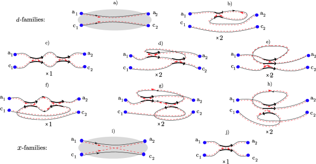
Figure 4: (a) Schematic graph of d-quadruplets, with the hatched area a “black box” containing any number of encounters; one of the dashed partner trajectories shares initial and final points with $\alpha$; the second partner trajectory similarly related to $\gamma$.
(b)-(h) d-quadruplets responsible for the leading-order contribution to the conductance variance. The diagrams (b), (f)-(h) containing encounters with antiparallel stretches exist only in the orthogonal case. A diagram may have a “twin” obtained by reflection in a horizontal line; the number of symmetric versions of each diagram is indicated by a multiplier underneath.
(i) Schematic graph of $x$-quadruplets, encounters suppressed: one of the partners shares initial link with $\gamma$ and final link with $\alpha$, the second one connects initial link of $\alpha$ with final link of $\gamma$. (j) An $x$-quadruplet involving one 2-encounter.

Off-diagonal contributions arise from quadruplets of trajectories differing in encounters; see Fig. 4 for examples. Each trajectory pair $(\alpha,\gamma)$ typically contains a huge number of encounters, where stretches of $\alpha$ and/or $\gamma$ come close to each other (up to time reversal). Partner trajectories $\beta$, $\delta$ can be obtained by switching connections within some encounters. Together, $\beta$ and $\delta$ go through the same links as $\alpha$ and $\gamma$, and traverse each $l$-encounter exactly $l$ times, just like the pair $(\alpha,\gamma)$. Consequently, the cumulative action of $(\beta,\delta)$ is close to the one of $(\alpha,\gamma)$, with a small action difference $\Delta S=(S_{\alpha}+S_{\gamma})-(S_{\beta}+S_{\delta})$ originating from the intra-encounter reconnections.

Different quadruplet families are distinguished by the number of $l$-encounters, the mutual orientation of encounter stretches, their distribution among $\alpha$ and $\gamma$, and the reconnections leading to $\beta$ and $\delta$. Similar as the diagonal quadruplets, some families of quadruplets involve one partner trajectory whose initial and final links practically coincide with those of $\alpha$ and the other one whose initial and final links coincide with those of $\gamma$. When these families are depicted schematically with encounters suppressed they all look the same and in fact like diagonal quadruplets (see Fig. 4a), for which reason we shall refer to them as “$d$-families”; examples are depicted in Figs. 4b-h. In analogy to the diagonal quadruplets, $d$-quadruplets contribute with altogether $N_{1}^{2}N_{2}^{2}+N_{1}N_{2}$ channel combinations. Of these, $N_{1}^{2}N_{2}^{2}$ arise when $\alpha$ and $\beta$ start and end alike since then the four channel indices involved are unrestricted; when $\alpha$ and $\delta$ start and end alike, $N_{1}N_{2}$ combinations arise since the channels are restricted as $a_{1}=c_{1},\,a_{2}=c_{2}$.

A second type of quadruplet families is drawn schematically in Fig. 4i: here one partner trajectory practically coincides at its beginning with $\alpha$ and at its end with $\gamma$; the other trajectory coincides at its beginning with $\gamma$ and at its end with $\alpha$. The simplest example of such an “$x$-family” involves just one 2-encounter, see Fig. 4j Schanz ; EssenShot ; not surprisingly, our schematic sketch strongly resembles that picture. Since quadruplets contribute to the conductance variance only if they connect channels as $\alpha,\beta:a_{1}\to a_{2}$ and $\gamma,\delta:c_{1}\to c_{2}$, $x$-families arise only if either the ingoing channels or the outgoing channels coincide. If the ingoing channels coincide, $a_{1}=c_{1}$, the trajectory coinciding initially with $\gamma$ and finally with $\alpha$ has the form $a_{1}=c_{1}\to a_{2}$ and may be chosen as $\beta$; the trajectory coinciding initially with $\alpha$ and finally with $\gamma$ is of the form $a_{1}=c_{1}\to c_{2}$ and may be chosen as $\delta$. If $a_{2}=c_{2}$, similar arguments hold, with $\beta$ and $\delta$ interchanged. Thus, $x$-families arise for $N_{1}N_{2}^{2}$ channel combinations with $a_{1}=c_{1}$, and for $N_{1}^{2}N_{2}$ combinations with $a_{2}=c_{2}$, altogether for $NN_{1}N_{2}$ possibilities.

We shall presently find that quadruplet families contribute to the conductance variance according to the same rules as do pairs to the mean conductance: Each link yields a factor $\frac{1}{N}$, each encounter a factor $-N$; moreover, we have to multiply with the number of channel combinations, i.e. $N_{1}^{2}N_{2}^{2}+N_{1}N_{2}$ for $d$-families and $NN_{1}N_{2}$ for $x$-families.

To justify these rules we consider a family with numbers of $l$-encounters given by $\vec{v}=(v_{2},v_{3},v_{4},\ldots)$. Again, $\vec{v}$ determines the total number of encounters $V(\vec{v})$ and the number of encounter stretches $L(\vec{v})$. The overall number of links is now given by $L(\vec{v})+2$, since there is one link preceding each of the $L(\vec{v})$ encounter stretches, and the two final links of $\alpha$ and $\gamma$ which do not precede any encounter stretch. Similarly as for trajectory pairs, we can determine a density $w(s,u)$ of stable and unstable separations; this density will be normalized such that integration over all $s,u$ belonging to an interval $(\Delta S,\Delta S+d\Delta S)$ of action differences $\Delta S$ yields the number of pairs $\beta,\delta$ differing from given $\alpha,\gamma$ such that the quadruplet $(\alpha,\beta,\gamma,\delta)$ belongs to a given family and the action difference is inside that interval. Using the same arguments as in Subsection II.3, one finds $w(s,u)$ as an integral over $\{\Omega^{L-V}\,\prod_{\sigma=1}^{V}t_{\rm enc}^{\sigma}(s,u)\}^{-1}$, with the integration running over the durations of all links, except the final links of $\alpha$ and $\gamma$. The integration range must be restricted such that all links (including the final ones) have positive durations. To evaluate the contribution of one family to the quadruple sum in (33), we may now replace the summation over $\beta$ and $\delta$ by integration over $w(s,u)$,

$$\big{\langle}({\rm tr}(tt^{\dagger}))^{2}\big{\rangle}\big{|}_{\rm fam}=\frac{1}{T_{H}^{2}}\left\langle\sum_{a_{1},c_{1}\atop a_{2},c_{2}}\int d^{L-V}s\;d^{L-V}u\sum_{\alpha:a_{1}\to a_{2}\atop\gamma:c_{1}\to c_{2}}|A_{\alpha}|^{2}|A_{\gamma}|^{2}w(s,u){\rm e}^{{\rm i}\sum_{\sigma,j}s_{\sigma j}u_{\sigma j}/\hbar}\right\rangle\,.$$ (36)

The sums over $\alpha$, $\gamma$ can be performed using the Richter/Sieber rule to ultimately get further integrals over the durations of the final links of $\alpha$ and $\gamma$, with an integrand involving the survival probability $\exp\{-\frac{N}{T_{H}}(\sum_{i=1}^{L+2}t_{i}+\sum_{\sigma=1}^{V}t_{\rm enc}^{\sigma}(s,u))\}$. We thus meet with link and encounter integrals of the same type as for the mean conductance. All powers of $T_{H}$ mutually again cancel, and we are left with a factor $\frac{1}{N}$ from each of the $L(\vec{v})+2$ links and a factor $-N$ from each of the $V(\vec{v})$ encounters which altogether give $\frac{(-1)^{V(\vec{v})}}{N^{L(\vec{v})-V(\vec{v})+2}}$. The summation over $a_{1},c_{1},a_{2},c_{2}$ yields the number of channel combinations mentioned.

If we denote by ${\cal N}_{d}(\vec{v})$, ${\cal N}_{x}(\vec{v})$ the numbers of $d$- and $x$-families associated to $\vec{v}$, the sum over all families with fixed $L(\vec{v})-V(\vec{v})=m$ involves the subsums

$$d_{m} = \sum_{\vec{v}}^{L(\vec{v})-V(\vec{v})=m}(-1)^{V(\vec{v})}{\cal N}_{d}(\vec{v})$$

$$x_{m} = \sum_{\vec{v}}^{L(\vec{v})-V(\vec{v})=m}(-1)^{V(\vec{v})}{\cal N}_{x}(\vec{v})$$ (37)

which allow to write the yield of all families as

$$\big{\langle}({\rm tr}(tt^{\dagger}))^{2}\big{\rangle}=(N_{1}^{2}N_{2}^{2}+N_{1}N_{2})\underbrace{\left(\frac{1}{N^{2}}+\sum_{m=1}^{\infty}\frac{d_{m}}{N^{m+2}}\right)}_{\equiv D}+NN_{1}N_{2}\underbrace{\sum_{m=1}^{\infty}\frac{x_{m}}{N^{m+2}}}_{\equiv X}\,,$$ (38)

with $D$ arising from $d$-families (including the diagonal contribution) and $X$ from $x$-families.

The coefficients $d_{m},x_{m}$ are obtained by counting families of quadruplets. That counting is an elementary task for small $m$. The coefficient $d_{1}$ accounts for families of $d$-quadruplets differing in one 2-encounter ($L=2$, $V=1$, $m=1$). In the unitary case there are no such families, i.e., $d_{1}=0$. In the orthogonal case, we must consider quadruplets with one partner trajectory differing from $\alpha$ in a 2-encounter, and one partner trajectory identical to $\gamma$, see Fig. 4b; the quadruplet thus contains one Richter/Sieber pair and one diagonal pair. A similar family of quadruplets involves one partner trajectory identical to $\alpha$, and one partner trajectory differing from $\gamma$ in a 2-encounter. We thus have $d_{1}=-2$.

The following coefficient $d_{2}$ is determined by $d$-quadruplets differing in two 2-encounters or in one 3-encounter, the latter quadruplets contributing with a negative sign. Some of these quadruplets fall into two pairs contributing to the average conductance. Quadruplets consisting of one diagonal pair and one pair contributing to the coefficient $c_{2}$ of the average conductance (see Fig. 2) yield a contribution $2c_{2}$ to $d_{2}$ (i.e., 0 in the unitary case and 2 in the orthogonal case); the factor 2 arises because either $\alpha$ or $\gamma$ may belong to the diagonal pair. In the orthogonal case, there is one further family of quadruplets consisting of two Richter/Sieber pairs. Finally, we must reckon with quadruplets that do not fall into two pairs contributing to the mean conductance, as depicted in Figs. 4c-e, for the unitary case. Two further families are obtained by “reflection”, i.e., interchanging $\alpha$ and $\gamma$ in Figs.  4d and 4e. Taking into account the negative sign for Fig. 4e and its reflected version, the respective contributions sum up to 1. In the orthogonal case, the additional families in Figs. 4f-h and the reflected versions of Fig. 4g and h yield a further summand 1. Altogether, we thus find $d_{2}=1$ in the unitary case and $d_{2}=2+1+1+1=5$ in the orthogonal case.

The most important family of $x$-quadruplets, see Fig. 4j, involves a parallel encounter between one stretch of $\alpha$ and one stretch of $\gamma$. This family, discovered in Schanz for quantum graphs, gives rise to a coefficient $x_{1}=-1$ for systems with or without time-reversal invariance.

With the coefficients $d_{1},d_{2},x_{1}$, the conductance variance (38) can be evaluated up to corrections of order $O(\frac{1}{N})$. The result

$$\big{\langle}({\rm tr}(tt^{\dagger}))^{2}\big{\rangle}-\big{\langle}{\rm tr}(tt^{\dagger})\big{\rangle}^{2}=\begin{cases}\frac{N_{1}^{2}N_{2}^{2}}{N^{4}}+{\cal O}\left(\frac{1}{N}\right)&\mbox{unitary case}\\ \frac{2N_{1}^{2}N_{2}^{2}}{N^{4}}+{\cal O}\left(\frac{1}{N}\right)&\mbox{orthogonal case}\,,\end{cases}$$ (39)

coincides with the random-matrix prediction (32). We note that Eq. (39) could ultimately be attributed only to the quadruplets shown in Fig. 4c-h, since all other contributions mutually cancel. (In particular, the contributions proportional to $N_{1}^{2}N_{2}^{2}$ from all $d$-quadruplets that consist of two pairs contributing to the conductance are cancelled by the squared average conductance. The term proportional to $N_{1}N_{2}$ in the diagonal approximation is compensated by the contribution of $x$-quadruplets as in Fig. 4j.)

To go beyond Eq. (39) (and to show that no terms were missed in Eq. (39)), we must systematically count families of $d$- and $x$-quadruplets with arbitrarily many encounters. Similar to the case of conductance this can be done by establishing relations between families of trajectory quadruplets and structures of periodic orbit pairs. For details see Appendix A; the results differ for the two universality classes.

In the unitary case we find

$$d_{m}=\begin{cases}0&\mbox{if $m$ odd}\\ 1&\mbox{if $m$ even\,,}\end{cases}\qquad x_{m}=\begin{cases}-1&\mbox{if $m$ odd}\\ 0&\mbox{if $m$ even\,.}\end{cases}$$ (40)

The total contributions of all $d$- and $x$-families (per channel combination) now read

$$D = \frac{1}{N^{2}}+\sum_{m+1}^{\infty}\frac{d_{m}}{N^{m+2}}=\frac{1}{N^{2}-1}$$

$$X = \sum_{m=1}^{\infty}\frac{x_{m}}{N^{m+2}}=-\frac{1}{N(N^{2}-1)}\,.$$ (41)

The resulting conductance variance

$$\big{\langle}({\rm tr}(tt^{\dagger}))^{2}\big{\rangle}-\big{\langle}{\rm tr}(tt^{\dagger})\big{\rangle}^{2}=\frac{N_{1}^{2}N_{2}^{2}}{N^{2}(N^{2}-1)}$$ (42)

agrees with the random-matrix prediction (32).

In the orthogonal case we have

$$d_{m}=(-1)^{m}\frac{3^{m}+1}{2},\quad x_{m}=(-1)^{m}\frac{3^{m}-1}{2}\,.$$ (43)

The contributions of $d$- and $x$-families per channel combination now read

$$D = \frac{1}{N^{2}}+\sum_{m=1}^{\infty}\frac{d_{m}}{N^{m+2}}=\frac{N+2}{N(N+1)(N+3)}\,,$$

$$X = \sum_{m=1}^{\infty}\frac{x_{m}}{N^{m+2}}=-\frac{1}{N(N+1)(N+3)}$$ (44)

and determine the variance in search as

$$\big{\langle}({\rm tr}(tt^{\dagger}))^{2}\big{\rangle}-\big{\langle}{\rm tr}(tt^{\dagger})\big{\rangle}^{2}=\frac{2N_{1}N_{2}(N_{1}+1)(N_{2}+1)}{N(N+1)^{2}(N+3)}\,,$$ (45)

again in agreement with (32). Thus, we have once more verified the universal behavior of individual chaotic cavities.

IV Shot noise

Our reasoning can be extended to a huge class of observables which are quartic in the transmission amplitudes and thus determined by $d$- and $x$-quadruplets as well. For a first example, we consider shot noise: Due to the discreteness of the elementary charge, the current flowing through a mesoscopic cavity fluctuates in time as $I(t)=\overline{I}+\delta I(t)$ where $\overline{I}$ denotes the average current. These current fluctuations, the so-called shot noise, remain in place even at zero temperature. They are usually characterized through the power Beenakker

$$P=4\int_{0}^{\infty}\overline{\delta I(t_{0})\delta I(t_{0}+t)}dt$$ (46)

where the overline indicates an average over the reference time $t_{0}$.

Using our semiclassical techniques, we proceed to showing that for chaotic cavities, the energy-averaged power of shot noise takes a universal form. Again, our treatment applies to individual cavities and yields an expansion to all orders in the inverse number of channels. That expansion turns out convergent and summable to a simple expression which subsequently to our prediction was checked to agree with random-matrix theory by Savin and Sommers Dima .

Following Büttiker Buettiker , we express the power of shot noise through the transition matrices $t$

$$\langle P\rangle=\langle{\rm tr}(tt^{\dagger})-{\rm tr}(tt^{\dagger}tt^{\dagger})\rangle\,;$$ (47)

here, $P$ is averaged over the energy and measured in units $\frac{2e^{3}|V|}{\pi\hbar}$ depending on the voltage $V$. While the average conductance $\langle{\rm tr}(tt^{\dagger})\rangle$ was already evaluated in Section II, the quartic term turns into a quadruple sum over trajectories similar to the conductance variance

$$\big{\langle}({\rm tr}(tt^{\dagger}tt^{\dagger}))\big{\rangle}=\left\langle\sum_{a_{1},c_{1}\atop a_{2},c_{2}}t_{a_{1}a_{2}}t_{c_{1}a_{2}}^{*}t_{c_{1}c_{2}}t_{a_{1}c_{2}}^{*}\right\rangle=\frac{1}{T_{H}^{2}}\left\langle\sum_{a_{1},c_{1}\atop a_{2},c_{2}}\;\sum_{\begin{subarray}{c}\alpha:\,a_{1}\to a_{2}\\ \beta:\,c_{1}\to a_{2}\\ \gamma:\,c_{1}\to c_{2}\\ \delta:\,a_{1}\to c_{2}\end{subarray}}A_{\alpha}A_{\beta}^{*}A_{\gamma}A_{\delta}^{*}{\rm e}^{{\rm i}(S_{\alpha}-S_{\beta}+S_{\gamma}-S_{\delta})/\hbar}\right\rangle\,;$$ (48)

the trajectories $\alpha$, $\beta$, $\gamma$, $\delta$ must now connect the ingoing channels $a_{1},c_{1}$ to the outgoing channels $a_{2},c_{2}$ as indicated in the summation prescription.

As a consequence, the possible channel combinations for $d$- and $x$-families of quadruplets are changed relative to the conductance variance. In the present case, $d$-quadruplets, with one partner trajectory coinciding at its beginning and end with $\alpha$, and the other partner trajectory doing the same with $\gamma$, contribute only if either the ingoing or the outgoing channels coincide. If the ingoing channels coincide, the partner trajectory connecting the same points as $\alpha$ is of the type $a_{1}=c_{1}\to a_{2}$ and may be taken as $\beta$, whereas the trajectory connecting the same points as $\gamma$ has the form $a_{1}=c_{1}\to c_{2}$ and may be chosen as $\delta$. If the outgoing channels coincide, similar arguments apply, with $\beta$ and $\delta$ interchanged. Thus, $d$-quadruplets contribute only for $N_{1}N_{2}^{2}+N_{1}^{2}N_{2}=NN_{1}N_{2}$ channel combinations. In this sense, they take the role played by $x$-quadruplets in case of the conductance variance.

In turn, $x$-quadruplets now contribute for all channel combinations. Moreover, if both the ingoing and the outgoing channels coincide, either of the two partner trajectories may be chosen as $\beta$ or $\delta$, meaning that the corresponding channel combinations have to be counted for a second time. Thus, $x$-quadruplets now contribute for altogether $N_{1}^{2}N_{2}^{2}+N_{1}N_{2}$ channel combinations, like $d$-quadruplets in case of the conductance variance.

We can simply interchange the multiplicity factors in our formula for $\langle({\rm tr}(tt^{\dagger}))^{2}\rangle$, Eq. (38), to get

$$\big{\langle}{\rm tr}(tt^{\dagger}tt^{\dagger})\big{\rangle}=NN_{1}N_{2}D+(N_{1}^{2}N_{2}^{2}+N_{1}N_{2})X$$ (49)

and thus

$$\langle P\rangle=\begin{cases}\frac{N_{1}^{2}N_{2}^{2}}{N(N^{2}-1)}&\text{unitary case}\\ \frac{N_{1}(N_{1}+1)N_{2}(N_{2}+1)}{N(N+1)(N+3)}&\text{orthogonal case}\,.\end{cases}$$ (50)

Eq. (50) extends the known random-matrix result Beenakker ,

$$\langle P\rangle=\begin{cases}\frac{N_{1}^{2}N_{2}^{2}}{N^{3}}+{\cal O}\Big{(}\frac{1}{N}\Big{)}&\text{unitary case}\\ \frac{N_{1}^{2}N_{2}^{2}}{N^{3}}+\frac{N_{1}N_{2}(N_{1}-N_{2})^{2}}{N^{4}}+{\cal O}\Big{(}\frac{1}{N}\Big{)}&\text{orthogonal case}\,,\end{cases}$$ (51)

to all orders in $\frac{1}{N}$, for individual chaotic cavities. We can, moreover, give an intuitive interpretation for the terms in (51). The diagonal contributions to $\langle{\rm tr}(tt^{\dagger})\rangle$ and $\langle{\rm tr}(tt^{\dagger}tt^{\dagger})\rangle$ both read $\frac{N_{1}N_{2}}{N}$ and therefore mutually cancel. The leading contribution, $\frac{N_{1}^{2}N_{2}^{2}}{N^{3}}$, arises from $d$-quadruplets differing in a single 2-encounter (see Fig. 4j). In the unitary case, there are no terms of order 1, since all related families require time-reversal invariance. In the orthogonal case, Richter/Sieber pairs yield a contribution $-\frac{N_{1}N_{2}}{N^{2}}$ to $\langle{\rm tr}(tt^{\dagger})\rangle$, from which we have to subtract two contributions to $\langle{\rm tr}(tt^{\dagger}tt^{\dagger})\rangle$, the term $-\frac{2N_{1}N_{2}}{N^{2}}$ accounting for $d$-quadruplets differing in a single antiparallel 2-encounter (see Fig. 4b), and a term $\frac{4N_{1}^{2}N_{2}^{2}}{N^{4}}$ arising from $x$-quadruplets contributing to $x_{2}=4$. The latter $x$-quadruplets may differ in two 2-encounters, as in Figs. 5a and 5b, or in one 3-encounter, as in Fig. 5c. From the examples in Fig. 5, further families are obtained by interchanging $\alpha$ and $\gamma$, interchanging the two leads (for Figs. 5a and 5c), or interchanging the pairs $(\alpha,\gamma)$ and $(\beta,\delta)$ (for Fig. 5b). Each of the Figs. 5a-c therefore represents altogether four families, whose contributions indeed sum up to $x_{2}=4(-1)^{2}+4(-1)^{2}+4(-1)=4$. Together with the contributions mentioned before, they combine to (51).

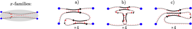
Figure 5: Families of $x$-quadruplets with $m=L-V=2$, contributing to the next-to-leading order of shot noise for time-reversal invariant systems.

V Current correlations in cavities with three leads

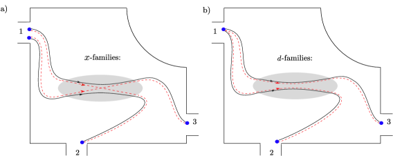
Figure 6: A cavity with three leads. If a voltage $V$ is applied between lead 1 and leads 2 and 3, one observes currents $I^{(1\to 2)}$ and $I^{(1\to 3)}$. As explained in the text, correlations between these currents are again determined by families of $d$- and $x$-quadruplets of trajectories.

Another interesting experimental setting involves a chaotic cavity with three leads, respectively supporting $N_{1}$, $N_{2}$ and $N_{3}$ channels; see Fig. 6. The second and the third lead are kept at the same potential, and a voltage is applied between these leads and the first one. Consequently, currents $I^{(1\to 2)}$, $I^{(1\to 3)}$ flow from the first lead to the second and third one. We shall be interested in the fluctuations $\delta I^{(1\to 2)}$, $\delta I^{(1\to 3)}$ of these currents around the corresponding averages values, and study correlations between $\delta I^{(1\to 2)}$ and $\delta I^{(1\to 3)}$ ThreeLeadL ; ThreeLeadB .

This setting is similar to the famous Hanbury Brown-Twiss experiment HBT in quantum optics: there, light from some source (corresponding to the first lead) was detected by two photomultipliers (corresponding to the second and third lead). Similar work on Fermions began somewhat later ThreeLeadL ; ThreeLeadB but the precise from of the correlation function is as yet unknown.

Our semiclassical reasoning can easily be extended to fill this gap. The two currents depend on the matrices $t^{(1\to 2)}$, $t^{(1\to 3)}$ containing the transition amplitudes between channels of the first and the second and third lead; these matrices have the sizes $N_{1}\times N_{2}$ and $N_{1}\times N_{3}$. As shown in ThreeLeadL ; ThreeLeadB , correlations between $\delta I^{(1\to 2)}$ and $\delta I^{(1\to 3)}$ are determined by the transition amplitudes as

$$4\int_{0}^{\infty}\overline{\delta I^{(1\to 2)}(t_{0})\delta I^{(1\to 3)}(t_{0}+t)}dt=-\big{\langle}{\rm tr}(t^{(1\to 2)}{t^{(1\to 2)}}^{\dagger}t^{(1\to 3)}{t^{(1\to 3)}}^{\dagger})\big{\rangle}\$$ (52)

(in units of $\frac{2e^{3}|V|}{\pi\hbar}$). Using the semiclassical expression for the transition amplitudes, we are again led to a sum over quadruplets of trajectories

$$\big{\langle}{\rm tr}(t^{(1\to 2)}{t^{(1\to 2)}}^{\dagger}t^{(1\to 3)}{t^{(1\to 3)}}^{\dagger})\big{\rangle}=\left\langle\sum_{\begin{subarray}{c}a_{1},c_{1}=1\ldots N_{1}\\ \quad\;a_{2}=1\ldots N_{2},\\ \quad\;c_{3}=1\ldots N_{3}\end{subarray}}t^{(1\to 2)}_{a_{1}a_{2}}{t^{(1\to 2)}_{c_{1}a_{2}}}^{*}t^{(1\to 3)}_{c_{1}c_{3}}{t^{(1\to 3)}_{a_{1}c_{3}}}^{*}\right\rangle$$

$$=\frac{1}{T_{H}^{2}}\left\langle\sum_{a_{1},c_{1},a_{2},c_{3}}\;\sum_{\begin{subarray}{c}\alpha:\,a_{1}\to a_{2}\\ \beta:\,c_{1}\to a_{2}\\ \gamma:\,c_{1}\to c_{3}\\ \delta:\,a_{1}\to c_{3}\end{subarray}}A_{\alpha}A_{\beta}^{*}A_{\gamma}A_{\delta}^{*}{\rm e}^{{\rm i}(S_{\alpha}-S_{\beta}+S_{\gamma}-S_{\delta})/\hbar}\right\rangle\,,$$ (53)

with $a_{1}$, $c_{1}$, $a_{2}$, $c_{3}$ labelling channels of the first, second and third lead, as indicated by the subscript. The trajectories $\alpha$, $\beta$, $\gamma$, $\delta$ must connect these channels as $\alpha(a_{1}\to a_{2})$, $\beta(c_{1}\to a_{2})$, $\gamma(c_{1}\to c_{3})$, $\delta(a_{1}\to c_{3})$.

The contribution of each family of trajectory quadruplets can be evaluated similarly to the conductance variance or shot noise. Since a particle can leave the cavity through any of the three leads, the escape rate depends on the overall number of channels $N=N_{1}+N_{2}+N_{3}$. Again, integration brings about factors $\frac{1}{N}$ and $-N$ for each link and each encounter. Only the numbers of channel combinations are changed. $x$-quadruplets as in Fig. 6a contribute for all $N_{1}^{2}N_{2}N_{3}$ possible choices of $a_{1}$, $c_{1}$, $a_{2}$, $c_{3}$. For any of these choices, partner trajectories connecting the initial point of $\gamma(c_{1}\to c_{3})$ to the final point of $\alpha(a_{1}\to a_{2})$, and the initial point of $\alpha$ to the final point of $\gamma$ are of the form $c_{1}\to a_{2}$ and $a_{1}\to c_{3}$ and can be chosen as $\beta$ and $\delta$, respectively. In contrast, $d$-quadruplets as in Fig. 6b contribute only for the $N_{1}N_{2}N_{3}$ combinations with coinciding ingoing channels $a_{1}=c_{1}$. For these combinations the partner trajectory coinciding at its ends with $\alpha$ is of the type $a_{1}=c_{1}\to a_{2}$ and can be taken as $\beta$ whereas the partner trajectory coinciding at its ends with $\gamma$ has the form $a_{1}=c_{1}\to c_{3}$ and can be chosen as $\delta$. With these numbers of channel combinations, the current correlations in a 3-lead geometry are obtained as

$$\langle{\rm tr}(t^{(1\to 2)}{t^{(1\to 2)}}^{\dagger}t^{(1\to 3)}{t^{(1\to 3)}}^{\dagger})\rangle=N_{1}N_{2}N_{3}D+N_{1}^{2}N_{2}N_{3}X=\begin{cases}\frac{N_{1}N_{2}N_{3}(N_{2}+N_{3})}{N(N^{2}-1)}&\text{unitary case}\\ \frac{N_{1}N_{2}N_{3}(N_{2}+N_{3}+2)}{N(N+1)(N+3)}&\text{orthogonal case}\,.\end{cases}$$ (54)

VI Ericson fluctuations

Another interesting quantum signature of chaos are so-called Ericson fluctuations, which have first been discovered experimentally in nuclear physics. In compound-nucleus reactions with strongly overlapping resonances, universal fluctuations in the correlation of two scattering cross sections at different energies have been observed. A first interpretation in terms of random-matrix theory was provided by Ericson Ericson and further theoretical investigations have been reported in VWZ , DB .

Later on, the relation between classical chaotic scattering and Ericson fluctuations in single-particle quantum mechanics has been discussed BS . Theoretical work shows that, e.g. the photoionization cross section of Rydberg atoms in external fields show universal correlations once the underlying classical dynamics is chaotic MainWunner .

Chaotic transport through a ballistic cavity displays Ericson fluctuations in the covariance of the conductance at two different energies,

$$\big{\langle}C(E,\epsilon)\big{\rangle}=\left\langle G(E)G\left(E+\frac{\epsilon N}{2\pi\overline{\rho}}\right)\right\rangle-\langle G\rangle^{2}\,,$$ (55)

with $G(E)={\rm tr}(tt^{\dagger})$. Here, the difference between the two energies was made dimensionless by referral to the energy scale $\frac{N}{2\pi\overline{\rho}}$ proportional to the number of channels and to the mean level spacing. Similarly as for the conductance variance, the semiclassical approximation (1) for $t(E),t(E^{\prime})$ where $E^{\prime}=E+\frac{\epsilon N}{2\pi\overline{\rho}}$ leads to a quadruple sum over trajectories,

$$\big{\langle}{\rm tr}\;tt^{\dagger}(E)\;\;{\rm tr}\;tt^{\dagger}(E^{\prime})\big{\rangle} = \left\langle\sum_{a_{1},c_{1}\atop a_{2},c_{2}}t_{a_{1}a_{2}}(E)t_{a_{1}a_{2}}^{*}(E)t_{c_{1}c_{2}}(E^{\prime})t_{c_{1}c_{2}}^{*}(E^{\prime})\right\rangle$$

$$= \frac{1}{T_{H}^{2}}\left\langle\sum_{a_{1},c_{1}\atop a_{2},c_{2}}\;\sum_{\begin{subarray}{c}\alpha,\beta:\,a_{1}\to a_{2}\\ \gamma,\delta:\,c_{1}\to c_{2}\end{subarray}}A_{\alpha}A_{\beta}^{*}A_{\gamma}A_{\delta}^{*}{\rm e}^{{\rm i}(S_{\alpha}(E)-S_{\beta}(E)+S_{\gamma}(E^{\prime})-S_{\delta}(E^{\prime}))/\hbar}\right\rangle\,,$$

the only difference to (33) being that the trajectories $\gamma$ and $\delta$ have to be taken at energy $E^{\prime}=E+\frac{\epsilon N}{2\pi\overline{\rho}}$. Using $\frac{\partial S_{\gamma}}{\partial E}=T_{\gamma}$, $\frac{\partial S_{\delta}}{\partial E}=T_{\delta}$, and $T_{H}=2\pi\hbar\overline{\rho}$, the phase factor can be cast into the form

$${\rm e}^{{\rm i}(S_{\alpha}(E)-S_{\beta}(E)+S_{\gamma}(E+\frac{\epsilon N}{2\pi\overline{\rho}})-S_{\delta}(E+\frac{\epsilon N}{2\pi\overline{\rho}}))/\hbar}\approx{\rm e}^{{\rm i}(S_{\alpha}(E)-S_{\beta}(E)+S_{\gamma}(E)-S_{\delta}(E))/\hbar}\times{\rm e}^{{\rm i}\frac{N}{T_{H}}\epsilon(T_{\gamma}-T_{\delta})}\,,$$ (57)

i.e., the quadruple sum in (VI) differs from (33) by an additional factor depending on the difference between the dwell times of $\gamma$ and $\delta$.

The latter difference may be written as a sum over links (with durations $t_{i}$) and encounters (with durations $t_{\rm enc}^{\sigma}$),

$$T_{\gamma}-T_{\delta}=\sum_{i=1}^{L+2}\eta_{i}t_{i}+\sum_{\sigma=1}^{V}\eta_{\sigma}t_{\rm enc}^{\sigma}\,.$$ (58)

Here, the integer numbers $\eta_{i}$ and $\eta_{\sigma}$ characterize the individual links and encounters. (Note the distinction between links and encounters by Latin and Greek subscripts). Each link occurs twice in the quadruplet, once in one of the original trajectories $\alpha,\gamma$ and then in one of the partner trajectories $\beta,\delta$. The number $\eta_{i}=0,\pm 1$ gives the difference between the numbers of times the $i$-th link is traversed by the trajectories $\gamma$ and $\delta$. We thus have $\eta_{i}=1$ if the $i$-th link is traversed by $\gamma$ and not by $\delta$, $i=0$ if it is traversed either by both or none of the two trajectories, and $i=-1$ if it is traversed only by $\delta$. Similarly, $\eta_{\sigma}$ gives the difference between the numbers of traversals of the $\sigma$-th encounter by $\gamma$ and $\delta$. For an $l$-encounter, $\eta_{\sigma}$ may range between $-l$ and $l$.

When evaluating the contribution of each family of quadruplets, Eq. (36), we simply have to add a phase factor ${\rm e}^{{\rm i}\frac{N}{T_{H}}\eta_{i}t_{i}}$ for each link, and a phase factor ${\rm e}^{{\rm i}\frac{N}{T_{H}}\eta_{\sigma}t_{\rm enc}^{\sigma}}$ for each encounter. The link and encounter integrals are thus replaced by

$$\int_{0}^{\infty}dt_{i}{\rm e}^{-\frac{N}{T_{H}}t_{i}}{\rm e}^{{\rm i}\frac{N}{T_{H}}\eta_{i}t_{i}}=\frac{T_{H}}{N(1-{\rm i}\eta_{i}\epsilon)}\,,$$ (59)

and

$$\left\langle\int d^{l-1}sd^{l-1}u\frac{1}{\Omega^{l-1}\,t_{\rm enc}^{\sigma}(s,u)}{\rm e}^{-\frac{N}{T_{H}}t_{\rm enc}(s,u)}{\rm e}^{{\rm i}\frac{N}{T_{H}}\eta_{\sigma}t_{\rm enc}(s,u)^{\sigma}}{\rm e}^{{\rm i}\sum_{j}s_{\sigma j}u_{\sigma j}/\hbar}\right\rangle=-\frac{N(1-{\rm i}\eta_{\sigma}\epsilon)}{T_{H}^{l-1}}\,.$$ (60)

As a consequence, our diagrammatic rules are modified to yield a factor $\frac{1}{N(1-{\rm i}\eta_{i}\epsilon)}$ for each link and a factor $-N(1-{\rm i}\eta_{\sigma}\epsilon)$ for each encounter.

We must, however, be aware that the numbers $\eta_{i},\eta_{\sigma}$ depend on which of the two partner trajectories is labelled as $\beta$ and which is labelled as $\delta$. Each family of $d$- or $x$-quadruplets hence comes with two different sets of numbers $\{\eta_{i},\eta_{\sigma}\}$, depending on the combinations of channels considered. For each $d$-family we have to keep into account $N_{1}^{2}N_{2}^{2}$ channel combinations with $\delta$ coinciding at its ends with $\gamma$; all these “$\delta\gamma$-type” combinations give rise to the same $\{\eta_{i},\eta_{\sigma}\}$ and to the same link and encounter factors. In addition, we must consider $N_{1}N_{2}$ combinations of the “$\delta\alpha$-type” with $\delta$ coinciding at its ends with $\alpha$, and a different set of $\{\eta_{i},\eta_{\sigma}\}$.

For each $x$-family we would, in principle, have to distinguish between $N_{1}N_{2}^{2}$ combinations with coinciding ingoing channels, and $\delta$ coinciding at its beginning with $\alpha$ and at its end with $\gamma$, and $N_{1}^{2}N_{2}$ combinations with coinciding outgoing channels, and $\delta$ coinciding at its beginning with $\gamma$ and at its end with $\alpha$. Such caution is, however, unnecessary for reasons of symmetry. Each $x$-family is accompanied by another one which is topologically mirror-symmetrical, with left and right in Fig. 4 interchanged. In this family, initial points turn into final ones, and vice versa, implying that $\beta$ and $\delta$ are interchanged. Since both families are taken into account simultaneously, “mistakes” like always choosing $\delta$ to connect the initial point of $\alpha$ to the final point of $\gamma$, are automatically compensated.

We can thus write the conductance covariance as

$$C(\epsilon)=N_{1}^{2}N_{2}^{2}\sum_{m=0}^{\infty}\frac{d_{m}^{\;(\delta\gamma)}}{N^{m+2}}+N_{1}N_{2}\sum_{m=0}^{\infty}\frac{d_{m}^{\;(\delta\alpha)}}{N^{m+2}}+N_{1}N_{2}N\sum_{m=1}^{\infty}\frac{x_{m}}{N^{m+2}}-\langle G\rangle^{2}$$ (61)

Here the coefficients $x_{m}(\epsilon),d_{m}^{\;(\delta\gamma)}(\epsilon),d_{m}^{\;(\delta\alpha)}(\epsilon)$ are the summary contributions of the $x$-quadruplets and the two mentioned groups of $d$-quadruplets, with $m=L(\vec{v})-V(\vec{v})-2$ (and thus $m=0$ for the diagonal quadruplets) and the denominator $N^{-m-2}$ dropped. The squared averaged conductance is $\epsilon$-independent and is determined by Eq. (2).

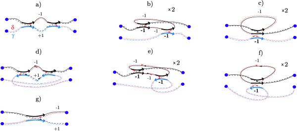
Figure 7: Families of trajectory quadruplets contributing to the covariance of conductance (coinciding with Fig.  4c-h,j). The trajectories $\gamma$ and $\delta$ are highlighted through dashing and dotting, assuming that $\delta$ connects the same points as $\gamma$. The picture also indicates all non-vanishing numbers $\eta_{i}$ and $\eta_{\sigma}$ (the latter in bold font).

The leading contribution to the conductance covariance corresponds to dropping in (61) all coefficients but $x_{1},d_{0}^{\;(\delta\gamma)},d_{0}^{\;(\delta\alpha)},d_{1}^{\;(\delta\gamma)},d_{2}^{\;(\delta\gamma)}$. For the conductance variance, we had seen that the contributions of $d$-quadruplets that fall into pairs ($\alpha$, $\beta$) and $(\gamma$, $\delta$) contributing to conductance cancel with the squared average conductance. The same remains valid here, since for these pairs $\gamma$ and $\delta$ traverse the same links and encounters, and all $\eta_{i}$ and $\eta_{\sigma}$ vanish. Again, the contributions of diagonal quadruplets $\alpha=\delta$, $\beta=\gamma$ and $x$-quadruplets as in Fig. 4j (see also Fig. 7g) mutually compensate; compared to the variance both kinds of quadruplets receive the same additional factors due to one link with $\eta_{i}=1$ (the trajectory $\beta=\gamma$ and the lower left link in Fig. 7g) and one link with $\eta_{i}=-1$ (the trajectory $\alpha=\delta$ and the upper left link in Fig. 7g).

Like for the conductance variance, the leading contribution to the covariance thus originates from the $d$-families in Fig. 4c-h which contain encounters between $\alpha$ and $\gamma$ and thus do not fall into pairs relevant for conductance. These families are redrawn in Fig. 7a-f, together with all non-vanishing numbers $\eta_{i}$ and $\eta_{\sigma}$. The trajectories $\gamma$ and $\delta$ are highlighted through dashing and dotting, assuming that $\delta$ connects the same points as $\gamma$; channel combinations with $\delta$ connecting the same points as $\alpha$ only contribute to higher orders in $\frac{1}{N}$. The family of Fig. 7a involves a link with $\eta_{i}=-1$ (the upper central one) and a link with $\eta_{i}=1$ (immediately below), and thus yields $\frac{N_{1}^{2}N_{2}^{2}(-N)^{2}}{N^{6}(1+{\rm i}\epsilon)(1-{\rm i}\epsilon)}=\frac{N_{1}^{2}N_{2}^{2}}{N^{4}(1+\epsilon^{2})}$. The same holds for the family in Fig. 7d, which requires time-reversal invariance. In contrast, the contributions of Fig. 7b,c,e, and f remain independent of $\epsilon$, since additional factors from links with $\eta_{i}=-1$ and encounters with $\eta_{\sigma}=-1$ mutually compensate; the same applies for the families represented by “$\times 2$” in Fig. 7, with ($\alpha$, $\beta$) and ($\gamma$, $\delta$) interchanged and the signs of $\eta_{i}$ and $\eta_{\sigma}$ flipped. As for the variance of conductance, the contributions of Fig. 7b,c,e,f thus mutually cancel, both in the orthogonal case and in the unitary case (where only Figs. 7b,c may exist). Altogether, we now obtain

$$\left\langle G(E)G\left(E+\frac{\epsilon N}{2\pi\overline{\rho}}\right)\right\rangle=\begin{cases}\frac{N_{1}^{2}N_{2}^{2}}{N^{4}(1+\epsilon^{2})}+{\cal O}\left(\frac{1}{N}\right)&\text{unitary case}\\ \frac{2N_{1}^{2}N_{2}^{2}}{N^{4}(1+\epsilon^{2})}+{\cal O}\left(\frac{1}{N}\right)&\text{orthogonal case}\,.\end{cases}$$ (62)

The Lorentzian form of (62) confirms the random-matrix predictions of Ericson .

Higher orders in $\frac{1}{N}$, not known from random-matrix theory, can be accessed by straightforward computer-assisted counting of families of quadruples differing in a larger number of encounters, or in encounters with more stretches. To do so, we generated permutations which describe possible structures of orbit pairs (see Appendix B and EssenFF ). We then “cut” through these pairs as described in Appendices A and B to obtain quadruplets of trajectories and determined the corresponding $\eta_{i}$, $\eta_{\sigma}$. The final result can be written as

$$\left\langle G(E)G\left(E+\frac{\epsilon N}{2\pi\overline{\rho}}\right)\right\rangle=\begin{cases}\frac{N_{1}^{2}N_{2}^{2}}{N^{4}}\left\{\frac{1}{(1+\epsilon^{2})}+\frac{1+3\epsilon^{2}+21\epsilon^{4}+5\epsilon^{6}+2\epsilon^{8}}{N^{2}\left(1+\epsilon^{2}\right)^{5}}\right\}\\ +{\cal O}\left(\frac{1}{N^{4}}\right)&\text{unitary case;}\\ \frac{2N_{1}^{2}N_{2}^{2}}{N^{4}\left(1+\epsilon^{2}\right)}+\frac{2N_{1}N_{2}}{N^{3}\left(1+\epsilon^{2}\right)}-\frac{2N_{1}^{2}N_{2}^{2}\left(5+12\epsilon^{2}+3\epsilon^{4}\right)}{N^{5}\left(1+\epsilon^{2}\right)^{3}}\\ -\frac{4N_{1}N_{2}}{N^{4}\left(1+\epsilon^{2}\right)^{3}}+\frac{2N_{1}^{2}N_{2}^{2}\left(18+78\epsilon^{2}+177\epsilon^{4}+48\epsilon^{6}+11\epsilon^{8}\right)}{N^{6}\left(1+\epsilon^{2}\right)^{5}}\\ +{\cal O}\left(\frac{1}{N^{3}}\right)&\text{orthogonal case}\,.\end{cases}$$ (63)

In the unitary case the $x$-type contribution cancels in all orders with the $d^{\;(\delta\alpha)}$-contribution; for that reason the overall result is proportional to $N_{1}^{2}N_{2}^{2}$.

VII Quantum transport in the presence of a weak magnetic field

VII.1 Changed diagrammatic rules

Our methods can also be applied to the case of a weak magnetic field, with a magnetic action of the order of $\hbar$. The necessary modifications were introduced in Nagao for the spectral form factor; see also JapanEssen . As in Nagao , we will obtain results interpolating between the orthogonal case (without a magnetic field) and the unitary case, where the magnetic field is strong enough to fully break time-reversal invariance. We shall assume that the field is too weak to influence the classical motion, meaning that we have to deal with the same families of trajectory pairs as in the orthogonal case. However, the action of each trajectory is increased by an amount proportional to the integral of the vector potential ${\bf A}$ along that trajectory, e.g., by

$$\Theta_{\alpha}=\int_{\alpha}\frac{e}{c}{\bf A}({\bf q})\cdot d{\bf q}\,,$$ (64)

for the trajectory $\alpha$. When we evaluate the average conductance, the action difference inside each pair of trajectories $\alpha$ and $\beta$ is thus increased by $\Theta_{\alpha}-\Theta_{\beta}$. This additional term may be neglected for pairs of trajectories where all encounters are parallel. For these pairs, all links and stretches of $\beta$ are close in phase space to links and stretches of $\alpha$, and therefore receive almost the same magnetic action.

The situation is different for pairs where $\alpha$ and $\beta$ traverse links or stretches with opposite sense of motion. Since the magnetic action changes sign under time reversal, such orbit pairs have significant magnetic action differences $\Theta_{\alpha}-\Theta_{\beta}$. These differences can be split into contributions from the individual links and encounters. Let us first consider links. If $\beta$ contains the time-reversed of the $i$-th link of $\alpha$, it must obtain the negative of the corresponding magnetic action $\Theta_{i}$. The difference $\Theta_{\alpha}-\Theta_{\beta}$ then receives a contribution $2\Theta_{i}$. Therefore we may write the contribution of each link as $2\mu_{i}\Theta_{i}$ with $\mu_{i}=1$ if the link changes direction on $\beta$ and $\mu_{i}=0$ otherwise.

Consider now the contribution of encounters. We assume that in the original trajectory $\alpha$ the encounter $\sigma$ had $\nu_{\sigma}$ stretches traversed in some direction (arbitrarily chosen as“positive”) meaning that the remaining $l_{\sigma}-\nu_{\sigma}$ stretches were traversed in the opposite, “negative” direction; in the trajectory partner $\beta$ these numbers will generally change to $\nu_{\sigma}^{\prime},l_{\sigma}-\nu_{\sigma}^{\prime}$ correspondingly. Denoting the magnetic action accumulated on a single stretch traversed in a positive direction by $\Theta_{\sigma}$ we see that the encounter $\sigma$ yields $2\mu_{\sigma}\Theta_{\sigma}$ to the magnetic action difference, with $\mu_{\sigma}=\nu_{\sigma}^{\prime}-\nu_{\sigma}$. The overall magnetic contribution to the action difference now reads

$$\Theta_{\alpha}-\Theta_{\beta}=\sum_{i=1}^{L+1}2\mu_{i}\Theta_{i}+\sum_{\sigma=1}^{V}2\mu_{\sigma}\Theta_{\sigma}$$ (65)

and yields a phase factor

$$\prod_{i=1}^{L+1}{\rm e}^{{\rm i}2\mu_{i}\Theta_{i}/\hbar}\prod_{\sigma=1}^{V}{\rm e}^{{\rm i}2\mu_{\sigma}\Theta_{\sigma}/\hbar}\,,$$ (66)

where we again distinguish between links and encounters only through Latin vs. Greek subscripts.

To handle this additional phase factor, we show that for fully chaotic (in particular, ergodic and mixing) dynamics, the magnetic action may effectively be seen as a random variable Nagao . For fully chaotic systems, any point on any trajectory can be located everywhere on the energy shell, with a uniform probability given by the Liouville measure. Moreover, phase-space points following each other after times larger than a certain classical “equilibration” time $t_{\rm cl}$ can be seen as uncorrelated. We will therefore split each link or encounter stretch into pieces of duration $t_{\rm cl}$. These pieces have different magnetic actions. Let us consider the probability density for these actions. Since positive and negative contributions to the magnetic action are equally likely, the expectation value for the action of an orbit piece must be equal to zero. The width $W$ (i.e., the square root of the variance $W^{2}$) must be proportional to the vector potential and therefore to the magnetic field $B$. Since the magnetic actions of the individual pieces are uncorrelated, the central limit theorem then implies that the magnetic actions of links with $K\equiv\frac{t_{i}}{t_{\rm cl}}\gg 1$ pieces obey a Gaussian probability distribution with the width $\sqrt{K}W$, i.e.,

$$P(\Theta_{i})=\frac{1}{\sqrt{2\pi KW^{2}}}{\rm e}^{-\frac{\Theta_{i}^{2}}{2KW^{2}}}$$ (67)

The phase factor arising from a link averages to $\int d\Theta_{i}P(\Theta_{i}){\rm e}^{{\rm i}2\mu_{i}\Theta_{i}/\hbar}={\rm e}^{-\mu_{i}bt_{i}}$, depending on the system-specific parameter $b=\frac{2KW^{2}}{\hbar^{2}t_{i}}=\frac{2W^{2}}{\hbar^{2}t_{\rm cl}}\propto\frac{B^{2}}{\hbar^{2}}$ and on $\mu_{i}=\mu_{i}^{2}\in\{0,1\}$. Similarly, the phase factor associated with the $\sigma$-th encounter averages to ${\rm e}^{-\mu_{\sigma}^{2}bt_{\rm enc}^{\sigma}}$ Nagao . Links and stretches traversed in opposite directions by $\alpha$ and $\beta$ thus lead to exponential suppression factors in the contributions of trajectory pairs.

These factors have to be taken into account when evaluating the average conductance, starting from (22). The link integrals are changed into

$$\int_{0}^{\infty}dt_{i}{\rm e}^{-\frac{N}{T_{H}}t_{i}}{\rm e}^{-\mu_{i}bt_{i}}=\frac{T_{H}}{N(1+\mu_{i}\xi)}\,,$$ (68)

with $\xi\equiv\frac{T_{H}}{N}b\propto\frac{B^{2}}{\hbar}$, whereas for each encounter we find an integral

$$\left\langle\int d^{l-1}sd^{l-1}u\frac{1}{\Omega^{l-1}\,t_{\rm enc}^{\sigma}(s,u)}{\rm e}^{-\frac{N}{T_{H}}t_{\rm enc}^{\sigma}(s,u)}{\rm e}^{-\mu_{\sigma}^{2}bt_{\rm enc}^{\sigma}(s,u)}{\rm e}^{{\rm i}\sum_{j}s_{\sigma j}u_{\sigma j}/\hbar}\right\rangle=-\frac{N(1+\mu_{\sigma}^{2}\xi)}{T_{H}^{l-1}}\,.$$ (69)

Since the $T_{H}$’s again mutually cancel, our diagrammatic rules are changed to give a factor $\frac{1}{N(1+\mu_{i}\xi)}$ for each link and a factor $-N(1+\mu_{\sigma}^{2}\xi)$ for each encounter; the arising product has to be multiplied with the number of channel combinations, i.e., $N_{1}N_{2}$ for the average conductance.

The same rules carry over to the conductance variance, shot noise, and correlations in a three-lead geometry. In these cases, $\mu_{i}$ is equal to 1 if the $i$-th link of the pair ($\alpha$, $\gamma$) is reverted in ($\beta$, $\delta$), and $\mu_{\sigma}$ counts the stretches of the $\sigma$-th encounter of ($\alpha$, $\gamma$) which are reverted in ($\beta$, $\delta$); the sign of $\mu_{\sigma}$ is fixed as above.

VII.2 Mean conductance

For the average conductance, the diagonal contribution, $\frac{N_{1}N_{2}}{N}$, remains unaffected by the magnetic field. The contribution of Richter/Sieber pairs, $-\frac{N_{1}N_{2}}{N^{2}}$, obtains an additional factor $\frac{1}{1+\xi}$, since one of the three links of $\alpha$ in Fig. 1 or 2a is traversed by $\beta$ in opposite sense. The next order originates from trajectory pairs as in Fig. 2b-j where arrows indicate the direction of motion inside the encounters and highlight those links which are traversed by $\alpha$ and $\beta$ with opposite sense of motion. The contributions of the families in Fig. 2b, c, d, g, i, j remain unchanged: In Fig. 2b, g no links or encounter stretches are reverted; for Fig. 2c, d, i, j the number of links with $\mu_{i}=1$ and encounters with $\mu_{\sigma}^{2}=1$ coincide, meaning that the $\xi$-dependent factors mutually compensate. The six above families cancel mutually due to the negative sign for Fig. 2g, i, j. The contributions of Fig. 2e, f, h obtain a factor $\frac{1}{(1+\xi)^{2}}$ from two reverted links; due to the negative sign of Fig. 2h, they sum up to $\frac{N_{1}N_{2}}{N^{3}(1+\xi)^{2}}$. We thus find

$$\langle{\rm tr}(tt^{\dagger})\rangle=\frac{N_{1}N_{2}}{N}\left\{1-\frac{1}{N(1+\xi)}+\frac{1}{N^{2}(1+\xi)^{2}}\right\}+{\cal O}\left(\frac{1}{N^{2}}\right)\,.$$ (70)

Counting further families of trajectory pairs with the help of a computer program one is able to proceed to rather high orders in $\frac{1}{N}$. We then find

$$\langle{\rm tr}(tt^{\dagger})\rangle=\frac{N_{1}N_{2}}{N}\Bigg{\{}1 - \frac{1}{N}\frac{1}{(1+\xi)}+\frac{1}{N^{2}}\frac{1}{(1+\xi)^{2}}-\frac{1}{N^{3}}\frac{1+2\xi+13\xi^{2}+4\xi^{3}+\xi^{4}}{(1+\xi)^{5}}+\frac{1}{N^{4}}\frac{1+2\xi+49\xi^{2}+4\xi^{3}+\xi^{4}}{(1+\xi)^{6}}$$ (71)

$$+ {\cal O}\left(\frac{1}{N^{5}}\right)\Bigg{\}}$$

As expected, (70) and (71) interpolate between the results for the orthogonal case, reached for $B\to 0$ and thus $\xi\to 0$, and the unitary case, formally reached for $B\to\infty$ and thus $\xi\to\infty$. The convergence to the unitary result is non-trivial: The contributions of the families in Fig. 2c,d,i,j are not affected by a magnetic field, because all $\xi$-dependent factors cancel. These contributions thus survive in the limit $\xi\to\infty$ (i.e., when the magnetic action becomes much larger than $\hbar$, but the trajectory deformations due to Lorentz force can still be disregarded), but vanish in the unitary case (i.e., when the magnetic field is strong enough to considerably deform the trajectories). The agreement between the limit $\xi\to\infty$ and the unitary result implies that the contributions of all such families must sum to zero, for all orders in $\frac{1}{N}$. Order by order, (71) coincides with the results of Weidenmueller , where the individual coefficients were given as (rather involved) random-matrix integrals.

VII.3 Conductance variance, shot noise and three-lead correlations

For observables determined by families of trajectory quadruplets, it is convenient to first evaluate the overall contributions of $d$- and $x$-families per channel combination. These contributions, denoted by $D$ and $X$, now depend on the parameter $\xi$. The contribution of $d$-families reads

$$D = \frac{1}{N^{2}}-\frac{2}{N^{3}(1+\xi)}+\frac{1}{N^{4}}\left[1+\frac{4}{(1+\xi)^{2}}\right]$$ (72)

$$+\frac{1}{N^{5}}\left[-\frac{10}{1+\xi}-\frac{4}{(1+\xi)^{3}}-\frac{2(1+4\xi)^{2}}{(1+\xi)^{5}}+\frac{2(1+9\xi)}{(1+\xi)^{4}}\right]+{\cal O}\left(\frac{1}{N^{6}}\right)\,,$$

generalizing our previous results (III.2) and (III.2) for the unitary and orthogonal cases. The leading term, originating from diagonal quadruplets, remains unaffected by the magnetic field. The second term is due to quadruplets as in Fig. 4b. Since in these quadruplets, one link of ($\alpha$, $\gamma$) is time-reversed in ($\beta$, $\delta$), the corresponding contribution is proportional to $\frac{1}{1+\xi}$. It is easy to check that the third term correctly accounts for $d$-quadruplets differing in two 2-encounters, or in one 3-encounter; compare Subsection III.2 and Fig. 4. The higher-order terms were again generated by a computer program.

In the overall contribution of $x$-families,

$$X=-\frac{1}{N^{3}}+\frac{4}{N^{4}(1+\xi)}+\frac{1}{N^{5}}\left[-1-\frac{10}{(1+\xi)^{2}}-\frac{2(1+4\xi)}{(1+\xi)^{4}}\right]+{\cal O}\left(\frac{1}{N^{6}}\right)\,,$$ (73)

the term $-\frac{1}{N^{3}}$ accounts for $x$-quadruplets differing in a parallel 2-encounter, Fig. 4j. These quadruplets are not affected by the magnetic field. All families responsible for the second term, Fig. 5a-c, display a Lorentzian field dependence $\frac{1}{1+\xi}$: While Figs. 5a and 5c contain one time-reversed link and only encounters with $\mu_{\sigma}=0$, Fig. 5b involves two time-reversed links and one encounter with $\mu_{\sigma}^{2}=1$. The remaining terms were again found with the help of a computer.

With these values of $D$ and $X$, we obtain, writing out only terms up to ${\cal O}(N^{-1})$,

• the conductance variance

  $$\big{\langle}({\rm tr}(tt^{\dagger}))^{2}\big{\rangle}-\big{\langle}{\rm tr}(tt^{\dagger})\big{\rangle}^{2}=\frac{N_{1}^{2}N_{2}^{2}}{N^{4}}\left(1+\frac{1}{(1+\xi)^{2}}\right)+-\frac{2N_{1}^{2}N_{2}^{2}(5+8\xi+4\xi^{2})}{N^{5}(1+\xi)^{3}}+\frac{2N_{1}N_{2}}{N^{3}(1+\xi)}+{\cal O}\left(\frac{1}{N^{2}}\right)\,,$$ (74)

• the power of shot noise

  $$\big{\langle}{\rm tr}(tt^{\dagger})-{\rm tr}(tt^{\dagger}tt^{\dagger})\big{\rangle}=\frac{N_{1}^{2}N_{2}^{2}}{N^{3}}+\frac{N_{1}N_{2}(N_{1}-N_{2})^{2}}{N^{4}(1+\xi)}+\frac{N_{1}^{2}N_{2}^{2}(13+32\xi+16\xi^{2}+4\xi^{3}+\xi^{4})}{N^{5}(1+\xi)^{4}}-\frac{3N_{1}N_{2}}{N^{3}(1+\xi)^{2}}+{\cal O}\left(\frac{1}{N^{2}}\right)\,,$$ (75)

• and current correlations for a cavity with three leads

  $$\langle{\rm tr}(t^{(1\to 2)}{t^{(1\to 2)}}^{\dagger}t^{(1\to 3)}{t^{(1\to 3)}}^{\dagger})\rangle=\frac{N_{1}N_{2}N_{3}(N_{2}+N_{3})}{N^{3}}+\frac{2N_{1}N_{2}N_{3}(N_{1}-N_{2}-N_{3})}{N^{4}(1+\xi)}$$

  $$+\frac{N_{1}N_{2}N_{3}\left[(N_{2}+N_{3})(1+\xi)^{2}(5+2\xi+\xi^{2})-2N_{1}(4+10\xi+3\xi^{2})\right]}{N^{5}(1+\xi)^{4}}+{\cal O}\left(\frac{1}{N^{2}}\right)\,.$$ (76)

At least the higher orders in $\frac{1}{N}$ are new results. In particular, for the power of shot noise, we do not only obtain the previously known cancellation of the second term at $N_{1}=N_{2}=\frac{N}{2}$, but also a new field dependence due to the third term,

$$\big{\langle}{\rm tr}(tt^{\dagger})-{\rm tr}(tt^{\dagger}tt^{\dagger})\big{\rangle}=\frac{N}{16}+\frac{1}{N}\frac{1+8\xi+4\xi^{2}+4\xi^{3}+\xi^{4}}{16(1+\xi)^{4}}+{\cal O}\Big{(}\frac{1}{N^{2}}\Big{)}\,;$$ (77)

VII.4 Ericson fluctuations

When studying Ericson fluctuations in a weak magnetic field, we have to deal with two parameters (apart from the channel numbers): the scaled energy difference $\epsilon$ and the parameter $\xi$ proportional to the squared magnetic field. Our diagrammatic rules are then changed in a straightforward way. Each link yields a factor $\frac{1}{N(1+\mu_{i}\xi-{\rm i}\eta_{\sigma}\epsilon)}$, whereas each encounter gives $-N(1+\mu_{\sigma}\xi-{\rm i}\eta_{\sigma}\epsilon)$, to be multiplied with the number of channel combinations.

As in the orthogonal and unitary cases, the leading contribution can be attributed to the quadruplets in Figs. 7a and 7d; all other contributions of the same or lower order, including the remaining families in Fig. 7, mutually cancel. Quadruplets as in Fig. 7a do not feel the magnetic field, and thus yield $\frac{N_{1}^{2}N_{2}^{2}}{N^{4}(1+\epsilon^{2})}$ as shown in Section VI; here we dropped lower-order corrections due to the case of coinciding channels. For the family of quadruplets depicted in Fig. 7d, the two links with $\eta_{i}=\pm 1$ connecting the two encounters are reversed inside ($\beta$, $\delta$) and thus have $\mu_{i}=1$. We obtain factors $\frac{1}{N(1+\xi-{\rm i}\epsilon)}$ and $\frac{1}{N(1+\xi+{\rm i}\epsilon)}$ from these two links, $\frac{1}{N}$ from each of the four remaining link, and $-N$ from the encounter. Multiplication with the number of channel combination yields a contribution $\frac{N_{1}^{2}N_{2}^{2}}{N^{4}((1+\xi)^{2}+\epsilon^{2})}$. Ericson fluctuations in a weak magnetic field are therefore determined as

$$\left\langle G(E)G\left(E+\frac{\epsilon N}{2\pi\overline{\rho}}\right)\right\rangle-\langle G\rangle^{2}=\frac{N_{1}^{2}N_{2}^{2}}{N^{4}}\left\{\frac{1}{1+\epsilon^{2}}+\frac{1}{(1+\xi)^{2}+\epsilon^{2}}\right\}+{\cal O}\left(\frac{1}{N}\right)\,.$$ (78)

VIII Conclusions

Contribution of each link	simplest case		$\frac{1}{N}$
	with energy diff.	$\propto\epsilon$ and squ. magn. field $\propto\xi$	$\frac{1}{N(1+\mu_{i}\xi-i\eta_{i}\epsilon)}$
Contribution of each encounter	simplest case		$-N$
	with energy diff.	$\propto\epsilon$ and squ. magn. field $\propto\xi$	$-{N(1+\mu_{\sigma}^{2}\xi-i\eta_{\sigma}\epsilon)}$
Total contribution	trajectory pairs	unitary case	$\frac{1}{N}$
per channel combination		orthogonal case	$\frac{1}{N+1}$
	$d$-quadruplets	unitary case	$\frac{1}{N^{2}-1}$
		orthogonal case	$\frac{N+2}{N(N+1)(N+3)}$
	$x$-quadruplets	unitary case	$-\frac{1}{N(N^{2}-1)}$
		orthogonal case	$-\frac{1}{N(N+1)(N+3)}$
Number of channel combinations	trajectory pairs	conductance	$N_{1}N_{2}$
	$d$-quadruplets	variance of conductance	$N_{1}^{2}N_{2}^{2}+N_{1}N_{2}$
		shot noise	$N_{1}N_{2}N$
		3-lead correlations	$N_{1}N_{2}N_{3}$
	$x$-quadruplets	variance of conductance	$N_{1}N_{2}N$
		shot noise	$N_{1}^{2}N_{2}^{2}+N_{1}N_{2}$
		3-lead correlations	$N_{1}^{2}N_{2}N_{3}$

Table 1: Diagrammatic rules determining chaotic quantum transport. The table shows link and encounter contributions for all observables discussed in the present paper. For the simplest cases (conductance, conductance variance, shot noise, 3-lead correlations), we have also listed the summed-up contributions of trajectory pairs and $d$- and $x$-quadruplets and the numbers of channel combinations.

A semiclassical approach to transport through chaotic cavities is established. We calculate mean and variance of the conductance, the power of shot noise, current fluctuations in cavities with three leads, and the covariance of the conductance at two different energies. These observables are dealt with for systems with and without a magnetic field breaking time-reversal invariance, as well as in the crossover between these scenarios caused by a weak magnetic field leading to a magnetic action of the order of $\hbar$. In contrast to random-matrix theory, our results apply to individual chaotic cavities, and do not require any averaging over ensembles of systems. Moreover, we go to all orders in the inverse number of channels.

Transport properties are expressed as sums over pairs or quadruplets of classical trajectories. These sums draw systematic contributions from pairs and quadruplets whose members differ by their connections in close encounters, and almost coincide in the intervening links. The contributions arising from the topologically different families of quadruplets or pairs are evaluated using simple and general diagrammatic rules, summarized in Tab. 1. (These rules remain in place even for observables involving higher powers of the transition matrix, as shown in Appendix C).

Our work shows that, under a set of conditions, individual chaotic systems demonstrate transport properties devoid of any system-specific features and coinciding with the RMT predictions. An obvious next stage would be investigation of the system-specific deviations from RMT observed when these conditions are not met. Previous work RS ; EssenCond ; EssenShot has already motivated an extension to the regime where the average dwell time $T_{D}$ is of the order of the Ehrenfest time $T_{E}$, i.e. the duration of the relevant encounters. Here, the semiclassical approach helped to settle questions controversial in the random-matrix literature EhrenfestRMT . As shown in Brouwer ; Whitney , the leading contributions to the average conductance and the power of shot noise become proportional to powers of ${\rm e}^{-T_{E}/T_{D}}$, ultimately arising from the exponential decay of the survival probability. On the other hand, the conductance variance turned out to be independent of $T_{E}$ Brouwer .

The door is open for a semiclassical treatment of many more transport phenomena, such as quantum decay Puhlmann , weak antilocalization Zaitsev , parametric correlations JapanEssen ; KuipersSieber , the full counting statistics of two-port cavities, and cavities with more leads. Extensions to the symplectic symmetry class, along the lines of Symplectic ; EssenFF , and to the seven new symmetry classes NewSymm (relevant e.g. for normal-metal/superconductor heterostructures or quantum chromodynamics) should be within reach. A generalization to quasi one-dimensional wires would finally lead to a semiclassical understanding of dynamical localization.

We are indebted to Dmitry Savin and Hans-Jürgen Sommers (who have reproduced our prediction (50) in random-matrix theory Dima ); to Piet Brouwer, Phillippe Jacquod, Saar Rahav, and Robert Whitney for friendly correspondence; to Taro Nagao, Alexander Altland, Ben Simons, Peter Silvestrov, and Martin Zirnbauer for useful discussions; to Austen Lamacraft for pointing us to OneChannel ; and to the Sonderforschungsbereich SFB/TR12 of the Deutsche Forschungsgemeinschaft and to the EPSRC for financial support.

Appendix A Trajectory quadruplets vs orbit pairs

In this Appendix we will establish a combinatorial method for counting families of trajectory quadruplets appearing in the theory of conductance variance and shot noise. We will see that trajectory quadruplets can be glued together to form orbit pairs, and orbit pairs can be cut into quadruplets of trajectories. In contrast to the case of trajectory pairs, see Fig. 2, we shall now need two cuts.

Our approach will be purely topological; e.g., an orbit pair $({\cal A},{\cal B})$ is regarded just as a pair of directed closed lines with links coinciding in ${\cal A}$ and ${\cal B}$ but differently connected in the encounters. Similarly, within each quadruplet $(\alpha,\beta,\gamma,\delta)$ we can assume that the links of $\alpha,\gamma$ exactly coincide with those of $\beta,\delta$. Mostly, we can even think of the quadruplets as black boxes with two left ports $a_{1},c_{1}$ and and two right ports $a_{2},c_{2}$. Regardless of the actual number of encounters inside, an $x$-quadruplet can then be treated like a “dressed” 2-encounter: connections $a_{1}$—$a_{2}$, $c_{1}$—$c_{2}$ in one of the trajectory pairs are replaced by $a_{1}$—$c_{2}$, $c_{1}$—$a_{2}$ in the partner pair, exactly as if a single 2-encounter existed between the trajectories $\alpha,\gamma$ of the quadruplet. On the other hand, no change in the connections occurs between the ports in a $d$-quadruplet, hence it is topologically equivalent to a pair of dressed links.

We shall consider both the unitary and the orthogonal case. In each case, we will use two slightly different methods to relate trajectory quadruplets and orbit pairs. This will allow us to express the quantities $x_{m}$ and $d_{m}$ defined in (III.2) through the auxiliary sums

$$A_{m} = \sum_{\vec{v}}^{M(\vec{v})=m}(-1)^{V(\vec{v})}(L(\vec{v})+1){\cal N}(\vec{v})$$

$$B_{m} = \sum_{\vec{v}}^{M(\vec{v})=m}(-1)^{V(\vec{v})}{\cal N}(\vec{v},2)\,,$$ (79)

where ${\cal N}(\vec{v})$ and ${\cal N}(\vec{v},2)$ are numbers of structures of orbit pairs (see Subsection II.4) and we have $M(\vec{v})\equiv L(\vec{v})-V(\vec{v})$; these auxiliary sums will be determined recursively in Subsection A.3 below.

A.1 Unitary case

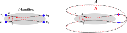
Figure 8: Left-hand side: Schematic picture of a $d$-quadruplet of trajectories $\alpha,\gamma$ (full lines), $\beta$, $\delta$ (dashed lines). Right-hand side: Outside the “bubble”, we added connection lines joining $(\alpha,\gamma)$ and $(\beta,\delta)$ into periodic orbits ${\cal A}$ and ${\cal B}$ with the initial link indicated by ”1.”. The additional lines of ${\cal A}$ and ${\cal B}$ coincide.

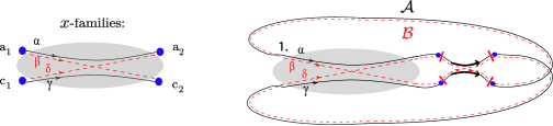
Figure 9: Left-hand side: Schematic picture of an $x$-quadruplet of trajectories $\alpha,\gamma$ (full lines), $\beta$, $\delta$ (dashed lines). Right-hand side: Outside the “bubble”, we added connection lines joining $(\alpha,\gamma)$ and $(\beta,\delta)$ into periodic orbits ${\cal A}$ and ${\cal B}$. The additional lines of ${\cal A}$ and ${\cal B}$ differ from each other, and can be viewed as an additional 2-encounter.

To illustrate method I, let us consider a $d$-quadruplet $(\alpha,\beta,\gamma,\delta)$, as on the left-hand side of Fig. 8, and merge $\alpha$ and $\gamma$ into one “orbit” ${\cal A}$. We connect the final point of $\alpha$ to the initial point of $\gamma$ and the final point of $\gamma$ to the initial point of $\alpha$, as shown on the right-hand side. Likewise, $\beta$ and $\delta$ can be glued together to an “orbit” ${\cal B}$. The connection lines added are the same for $(\alpha,\gamma)$ and for $(\beta,\delta)$: one connection line joins the coinciding final links of $\alpha$ and $\beta$ with the coinciding initial links of $\gamma$ and $\delta$, whereas the second one joins the final links of $\gamma$ and $\delta$ with the initial links of $\alpha$ and $\beta$. The orbits ${\cal A}$ and ${\cal B}$ differ in the same encounters as $(\alpha,\gamma)$ and $(\beta,\delta)$. To fix one structure for the orbit pair ${\cal A},{\cal B}$, we have to single out one link as the “first” and choose as such the link of ${\cal A}$ created by merging the final link of $\gamma$ with the initial link of $\alpha$ (indicated by ”1.” in Fig. 8).

We can revert the above procedure, to obtain families of $d$-quadruplets from structures of orbit pairs. We first have to cut both orbits inside the “initial” link. This leads to a trajectory pair with $L(\vec{v})+1$ rather than $L(\vec{v})$ links. We then have $L(\vec{v})+1$ choices for placing a second cut in any of these links. In each case, we end up with a trajectory quadruplet. Within this quadruplet, the trajectories following the first cut through ${\cal A}$ and ${\cal B}$ are labelled by $\alpha$ and $\beta$; the remaining ones are called $\gamma$ and $\delta$. In this way, each of the ${\cal N}(\vec{v})$ structures of orbit pairs related to a given $\vec{v}$ gives rise to $L(\vec{v})+1$ families of $d$-quadruplets with the same $\vec{v}$. The quantities ${\cal N}_{d}(\vec{v})$ and $d_{m}$ characterizing the $d$-families in (III.2) thus become accessible as

$${\cal N}_{d}(\vec{v}) = (L(\vec{v})+1){\cal N}(\vec{v})\,,$$ (80)

$$d_{m} = \sum_{\vec{v}}^{L(\vec{v})-V(\vec{v})=m}(-1)^{V(\vec{v})}(L(\vec{v})+1){\cal N}(\vec{v})=A_{m}\,.$$ (81)

Let us discuss a few examples. According to (81) the coefficient $d_{1}$ is determined by orbit pairs with $m=1$ (i.e., only one 2-encounter). Since in the unitary case there are no such orbit pairs, we have $d_{1}=0$. The following coefficient $d_{2}$ is determined by orbit pairs with $m=2$. In the unitary case there are only two such structures, ppi and pc (Fig. 2b and g). All quadruplets responsible for the coefficient $d_{2}$ can be obtained by making two cuts through these orbit pairs, one through the initial link which may be chosen arbitrarily. The second cut can go through any link; in particular, there are two possibilities for the second cut in the initial link, before and after the first cut. That means $L+1$=5 possible positions of the second cut for ppi. These lead to the quadruplets as in Fig. 4c and d, the reflected version of Fig. 4d, and quadruplets where either $\alpha$ or $\gamma$ contain two 2-encounters and the other trajectory contains none. For pc there are four possible positions for the second cut, corresponding to Fig. 4e, its reflected version, and quadruplets where either $\alpha$ or $\gamma$ contain the full 3-encounter. All quadruplet families related to a given structure make the same contributions $(-1)^{V}$ to the coefficient $d_{2}$, i.e., 1 for those obtained from ppi and -1 for those obtained from pc; we again see that $d_{2}=5-4=1$.

To explain method II, let us now consider $x$-quadruplets as on the left-hand side in Fig. 9. On the right-hand side, $\alpha$ and $\gamma$ are again merged into a periodic orbit ${\cal A}$, and $\beta$ and $\delta$ are once more merged into ${\cal B}$, by connection lines leading from the end of one trajectory to the beginning of the other one. In contrast to the first scenario, the pair $({\cal A},{\cal B})$ has one further 2-encounter between these lines, with different connections for the two partner orbits. To fix one structure for the latter orbit pair, we take the initial link of $\alpha$ as the “first” link of the orbit pair. This link is preceded by a “final” stretch, which must belong to the added 2-encounter. We must therefore reckon with orbit pairs associated to the vector $\vec{v}^{[\to 2]}$ and whose final stretches belong to a 2-encounter. In the notation of Subsection II.4, the number of structures of such orbit pairs is given by ${\cal N}(\vec{v}^{[\to 2]},2)$.

Each of these structures can be turned back into one family of $x$-quadruplets, by cutting out the added 2-encounter. Consequently, there is a one-to-one relation between $x$-families and the structures of orbit pairs considered. The number of $x$-families related to $\vec{v}$ and the coefficients $x_{m}$ defined in (III.2) are given by

$${\cal N}_{x}(\vec{v}) = {\cal N}(\vec{v}^{[\to 2]},2)\,,$$ (82)

$$x_{m} = \sum_{\vec{v}}^{L(\vec{v})-V(\vec{v})=m}(-1)^{V(\vec{v})}{\cal N}(\vec{v}^{[\to 2]},2)\,.$$ (83)

Rather than over $\vec{v}$, we may sum over $\vec{v}^{\prime}\equiv\vec{v}^{[\to 2]}$ with $L(\vec{v}^{\prime})-V(\vec{v}^{\prime})=(L(\vec{v})+2)-(V(\vec{v})+1)=m+1$. While the latter sum should be restricted to $\vec{v}^{\prime}$ with $v_{2}^{\prime}>0$, that restriction may be ignored since $\vec{v}^{\prime}$ with $v_{2}^{\prime}=0$ have ${\cal N}(\vec{v}^{\prime},2)=0$. Using $(-1)^{V(\vec{v}^{\prime})}=-(-1)^{V(\vec{v}^{\prime})}$ and dropping the primes we can express the coefficient $x_{m}$ as

$$x_{m}=-\sum_{\vec{v}}^{L(\vec{v})-V(\vec{v})=m+1}(-1)^{V(\vec{v})}{\cal N}(\vec{v},2)=-B_{m+1}\,.$$ (84)

For instance, the coefficient $x_{1}$ is determined by orbit pairs with $L(\vec{v})-V(\vec{v})=2$. Only one such structure (ppi) contains 2-encounters and yields a contribution $-1$, whereas pc involves only one 3-encounter. We thus find $x_{1}=-1$, as already seen previously.

Taken together, Eqs. (81), (84), and (26) indeed relate the conductance variance to structures of orbit pairs.

A.2 Orthogonal case

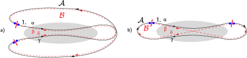
Figure 10: Sketches of orbit pairs $({\cal A},{\cal B})$. Inside the bubbles: quadruplets of trajectories obtained by cutting $({\cal A},{\cal B})$ in the initial link (indicated by ”1.”), and in one further link. In (a) both links are traversed by ${\cal A}$ and ${\cal B}$ with the same sense of motion, and the trajectory quadruplet is of type $d$. In (b), the second cut is placed in a link traversed with opposite senses of motion, and the resulting quadruplet is of type $x$.

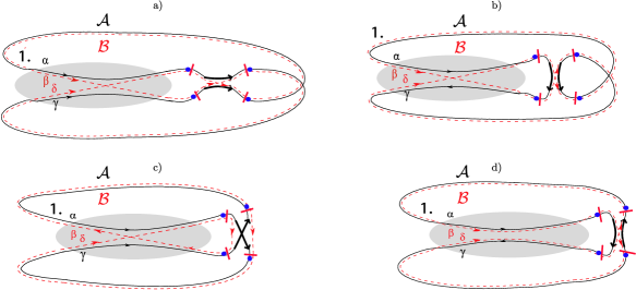
Figure 11: Sketches of orbit pairs $({\cal A},{\cal B})$ with one 2-encounter singled out. This 2-encounter contains the “final” encounter stretch, and is either (a) parallel in both ${\cal A}$ and ${\cal B}$, (b) parallel in ${\cal A}$ and antiparallel in ${\cal B}$, (c) antiparallel in ${\cal A}$ and parallel in ${\cal B}$, or (d) antiparallel in both ${\cal A}$ and ${\cal B}$.

For time-reversal invariant systems, we must now consider pairs of orbits ${\cal A}$, ${\cal B}$ differing in encounters whose stretches are either close or almost mutually time-reversed. The sense of traversal of an orbit now being arbitrary we fix the direction of ${\cal B}$ such that ${\cal B}$ traverses the “initial” link of ${\cal A}$ in the same direction.

We start with method I, i.e., we cut an orbit pair $({\cal A},{\cal B})$ inside links, first inside the initial link and afterwards in an arbitrary link. We have to distinguish two cases, respectively leading to $d$- and $x$-quadruplets. First assume that the second cut is placed in a link traversed by ${\cal A}$ and ${\cal B}$ with the same sense of motion; see Fig. 8 or 10a. As in the unitary case we then obtain a $d$-quadruplet of trajectories; this quadruplet is highlighted by a grey “bubble” in Fig. 8 and 10a, without depicting the encounters. Inside this quadruplet, $\alpha$ is defined as the trajectory following the cut through the initial link (marked by ”1.” in Fig. 8-11).

Now assume that the second cut is placed in a link traversed by ${\cal A}$ and ${\cal B}$ with opposite senses of motion. The resulting quadruplet, shown in the grey bubble in Fig. 10b, resembles an $x$-quadruplet, apart from the directions of motion. To obtain a true $x$-quadruplet, one has to revert the directions of motion of two trajectories in Fig. 10b, such that all trajectories point in the same direction as $\alpha$ (i.e., the trajectory following the cut inside the initial link).

We hence obtain the following relation between orbit pairs and trajectory quadruplets: By cutting inside links, each of the ${\cal N}(\vec{v})$ structures of orbit pairs related to $\vec{v}$ can be turned into a family of trajectory quadruplets in $L(\vec{v})+1$ possible ways. Through such cuts, all ${\cal N}_{d}(\vec{v})$ $d$-families and all ${\cal N}_{x}(\vec{v})$ $x$-families are obtained exactly once, since each $d$- or $x$-family could be inserted inside the bubble in Fig. 10a or 10b, respectively. We thus have

$$(L(\vec{v})+1){\cal N}(\vec{v})={\cal N}_{d}(\vec{v})+{\cal N}_{x}(\vec{v})\,$$ (85)

and summation as in the unitary case leads to

$$A_{m}=d_{m}+x_{m}$$ (86)

with $A_{m}$ defined in (A) and $d_{m}$, $x_{m}$ defined in (III.2).

We now turn to method II (cutting inside 2-encounters). We consider orbit pairs ${\cal A},{\cal B}$ containing one more 2-encounter compared with the quadruplets in question, assuming that the final encounter stretch of the orbits belongs to the “added” 2-encounter; the number of these structures is ${\cal N}(\vec{v}^{[\to 2]},2)$. Cutting out the added 2-encounter will create all possible quadruplets associated to $\vec{v}$, some of them, as we shall see, in several copies.

The added 2-encounter can be either parallel or antiparallel in the orbit ${\cal A}$ as well as in its partner ${\cal B}$. This leads to four different possibilities, depicted by arrows on white background in Fig. 11a-d. First suppose that the encounter in question is antiparallel in both ${\cal A}$ and ${\cal B}$, as in Fig. 11d. This is possible only if the ports of this encounter are connected in the same way in ${\cal A}$ and ${\cal B}$, up to time reversal; one can easily check that all other connections would lead to either ${\cal A}$ or ${\cal B}$ decomposing into several disjoint orbits. The connections outside the encounter, as depicted in the bubble in Fig. 11d, thus resemble $d$-quadruplets and can be turned into true $d$-quadruplets if we revert the sense of motion on some trajectories. Any $d$-family could be substituted for the bubble in Fig. 11d. Thus, cutting through 2-encounters of the kind in Fig. 11d produces all possible families of $d$-quadruplets.

In the three other cases, Fig. 11a-c, the remaining connections have to be of type $x$, up to the sense of motion on some trajectories, since connections of type $d$ would lead to decomposing orbits. To better understand these cases, it is helpful to view the corresponding $x$-quadruplets as a “dressed” 2-encounters. Then, the orbit pairs of Fig. 11a-c are topologically equivalent to the simple diagrams in Fig. 2. The orbit pair in Fig. 11a is of the type ppi whereas the pairs in Fig. 11b and c are both of the type api. (In Fig. 11b the initially parallel encounter is identified with the added encounter, and the initially antiparallel encounter is identified with the $x$-quadruplet, whereas the situation is opposite in Fig. 11c.) Any family of type $x$ could be substituted for the bubbles in each of the Figs. 11a-c, and can therefore be obtained by cutting three different structures of orbit pairs.

We have thus seen that by cutting through 2-encounters of the ${\cal N}(\vec{v}^{[\to 2]},2)$ structures of orbit pairs considered, we obtain each family of $d$-quadruplet once and once only, whereas each $x$-family is produced by three different structures. We therefore have

$${\cal N}(\vec{v}^{[\to 2]},2)={\cal N}_{d}(\vec{v})+3{\cal N}_{x}(\vec{v})\,,$$ (87)

and, by summing over $\vec{v}$ as in Subsection A.1,

$$-B_{m+1}=d_{m}+3x_{m}\,.$$ (88)

Eqs. (86) and (88) form a system of equations for the coefficients $d_{m}$, $x_{m}$, with the solution

$$d_{m} = \frac{3}{2}A_{m}+\frac{1}{2}B_{m+1}$$ (89a)

$$x_{m} = -\frac{1}{2}A_{m}-\frac{1}{2}B_{m+1}$$ (89b)

A.3 Recursion relations

We must calculate the auxiliary sums $A_{m},B_{m}$ defined in (A) for both the unitary and the orthogonal cases. We start from the recursion for the number of structures ${\cal N}(\vec{v})$ already used to evaluate the average conductance in Subsection II.4

$${\cal N}(\vec{v},2)-\sum_{k\geq 2}{\cal N}(\vec{v}^{[k,2\to k+1]},k+1)=\left(\frac{2}{\beta}-1\right){\cal N}(\vec{v}^{[2\to]})\,;$$ (90)

see Eq. (27). This time, (90) has to be multiplied not with $(-1)^{V(\vec{v})}$, but with $(-1)^{V(\vec{v})}L(\vec{v})=-(-1)^{V(\vec{v}^{[k,2\to k+1]})}(L(\vec{v}^{[k,2\to k+1]})+1)=-(-1)^{V(\vec{v}^{[2\to]})}(L(\vec{v}^{[2\to]})+2)$. If we subsequently sum over all $\vec{v}$ with $M(\vec{v})=m$, our recursion turns into

$$\sum_{\vec{v}}^{M(\vec{v})=m}\left\{(-1)^{V(\vec{v})}L(\vec{v}){\cal N}(\vec{v},2)+\sum_{k\geq 2}(-1)^{V(\vec{v}^{[k,2\to k+1]})}(L(\vec{v}^{[k,2\to k+1]})+1){\cal N}(\vec{v}^{[k,2\to k+1]},k+1)\right\}$$

$$=-\left(\frac{2}{\beta}-1\right)\sum_{\vec{v}}^{M(\vec{v})=m}(-1)^{V(\vec{v}^{[2\to]})}(L(\vec{v}^{[2\to]})+2){\cal N}(\vec{v})\,.$$ (91)

Changing the summation variables as in Subsection II.4, we find

$$\sum_{\vec{v}}^{M(\vec{v})=m}\left\{(-1)^{V(\vec{v})}L(\vec{v}){\cal N}(\vec{v},2)+\sum_{k\geq 2}(-1)^{V(\vec{v})}(L(\vec{v})+1){\cal N}(\vec{v},k+1)\right\}$$

$$=-\left(\frac{2}{\beta}-1\right)\sum_{\vec{v}}^{M(\vec{v})=m-1}(-1)^{V(\vec{v})}(L(\vec{v})+2){\cal N}(\vec{v})\,.$$ (92)

Using ${\cal N}(\vec{v},2)+\sum_{k\geq 2}{\cal N}(\vec{v},k+1)={\cal N}(\vec{v})$, we can simplify the left-hand side to $\sum_{\vec{v}}^{M(\vec{v})=m}(-1)^{V(\vec{v})}(L(\vec{v})+1){\cal N}(\vec{v})-\sum_{\vec{v}}^{M(\vec{v})=m}(-1)^{V(\vec{v})}{\cal N}(\vec{v},2)=A_{m}-B_{m}$, whereas the right-hand side turns into $-\left(\frac{2}{\beta}-1\right)(A_{m-1}+c_{m-1})$ with $c_{m-1}=\sum_{\vec{v}}^{M(\vec{v})=m-1}(-1)^{V(\vec{v})}{\cal N}(\vec{v})$, see Eq. (25). We thus find a first relation between $A_{m}$ and $B_{m}$,

$$A_{m}-B_{m}=-\left(\frac{2}{\beta}-1\right)(A_{m-1}+c_{m-1})\,.$$ (93)

A second relation between $A_{m}$ and $B_{m}$ follows from the recursion EssenFF

$${\cal N}(\vec{v},3)-\sum_{k\geq 2}{\cal N}(\vec{v}^{[k,3\to k+2]},k+2)=2\left(\frac{2}{\beta}-1\right){\cal N}(\vec{v}^{[3\to 2]},2)+\frac{2}{\beta}(L(\vec{v}^{[3\to]})+1){\cal N}(\vec{v}^{[3\to]})\,,$$ (94)

which has to be multiplied with $(-1)^{V(\vec{v})}=-(-1)^{V(\vec{v}^{[k,3\to k+2]})}=(-1)^{V(\vec{v}^{[3\to 2]})}=-(-1)^{V(\vec{v}^{[3\to]})}$ and summed over all $\vec{v}$ with $M(\vec{v})=m$. It is easy to see that the changed vectors $\vec{v}^{[k,2\to k+1]},\vec{v}^{[3\to 2]},\vec{v}^{[3\to]}$ in the arguments of ${\cal N}$ have $M(\vec{v}^{[k,3\to k+2]})=m$, $M(\vec{v}^{[3\to 2]})=m-1$, and $M(\vec{v}^{[3\to]})=m-2$. Again transforming the sums over $\vec{v}$ into sums over the arguments of ${\cal N}$, we are led to

$$\sum_{\vec{v}}^{M(\vec{v})=m}(-1)^{V(\vec{v})}\left\{{\cal N}(\vec{v},3)+\sum_{k\geq 2}{\cal N}(\vec{v},k+2)\right\}$$

$$=2\left(\frac{2}{\beta}-1\right)\sum_{\vec{v}}^{M(\vec{v})=m-1}(-1)^{V(\vec{v})}{\cal N}(\vec{v},2)-\frac{2}{\beta}\sum_{\vec{v}}^{M(\vec{v})=m-2}(-1)^{V(\vec{v})}(L(\vec{v})+1){\cal N}(\vec{v})\,.$$ (95)

Eq. (A.3) can be simplified if we use ${\cal N}(\vec{v},3)+\sum_{k\geq 2}{\cal N}(\vec{v},k+2)={\cal N}(\vec{v})-{\cal N}(\vec{v},2)$, and recall the definitions of $A_{m}$, $B_{m}$ and $c_{m}$, to get

$$c_{m}-B_{m}=2\left(\frac{2}{\beta}-1\right)B_{m-1}-\frac{2}{\beta}A_{m-2}$$ (96)

A.4 Results

In the unitary case the two relations between $A_{m}$ and $B_{m}$, Eqs. (93) and (96) yield a recursion for both quantities. In the unitary case, $\frac{2}{\beta}-1=0$, $c_{m}=0$, the two equations simplify to

$$A_{m}-B_{m}=0,\qquad-B_{m}=-A_{m-2}\,,$$ (97)

i.e., $A_{m}$ and $B_{m}$ coincide and depend only on whether $m$ is even or odd. Since in the unitary case $d_{m}=A_{m},\,x_{m}=-B_{m+1}$, see (81), and since the initial values $d_{1}=0,d_{2}=1$ are already established, we come to the expressions (40) for $x_{m},d_{m}$.

In the orthogonal case $\frac{2}{\beta}-1=1$, $c_{m}=(-1)^{m}$, Eqs. (93) and (96) take the form

$$A_{m}-B_{m} = -A_{m-1}+(-1)^{m}$$ (98a)

$$(-1)^{m}-B_{m} = 2B_{m-1}-2A_{m-2}\,.$$ (98b)

Eliminating $B_{m}$ and $B_{m-1}$ in (98b) with the help of (98a), we find a recursion for $A_{m}$,

$$A_{m}=-3A_{m-1}\,.$$ (99)

An initial condition is provided by $A_{1}=-3$, which accounts for the Richter/Sieber family of trajectory pairs with one 2-encounter, $V=1$, $L=2$ and $m=1$. We thus obtain

$$A_{m}=(-3)^{m},\qquad B_{m}\stackrel{{\scriptstyle\mbox{(\ref{orth1})}}}{{=}}A_{m}+A_{m-1}+(-1)^{m-1}=(-1)^{m}(2\cdot 3^{m-1}-1)\,.$$ (100)

After that, using (89a), (89b) we arrive at the result (43) of the main text.

Appendix B An algorithm for counting trajectory pairs and quadruplets

In our approach transport properties phenomena are related to trajectory pairs or quadruplets differing in encounters; we showed that all topologically different families of pairs or quadruplets can be found using the corresponding structures of orbit pairs considered in the theory of spectral fluctuations EssenFF . The number of structures to be considered grows exponentially with the order of approximation, and in absence of an analytic formula (in particular, for Ericson fluctuations or crossover in a magnetic field) can be evaluated only with the help of a computer. Here we describe an algorithm for the systematic generation of orbit pairs.

Assume time-reversal invariant dynamics, and let $\mathcal{A}$ be a periodic orbit and $\mathcal{B}$ its partner obtained by reconnections in a set of encounters associated to the vector $\vec{v}=\left(v_{2},v_{3},v_{4},\ldots\right)$. Let us then number all the $L=L(\vec{v})$ encounter stretches in $\mathcal{A}$ in order of traversal. Each encounter has two sides which can be arbitrarily named left and right such that the two ends of the $i$ -th encounter stretch can be called its left ($i_{l}$) and right ($i_{r}$) ports. The direction of traversal of the encounter stretches in $\mathcal{A}$ will be denoted by another vector $\overrightarrow{\sigma}=\left(\sigma_{1}\sigma_{2}\ldots\sigma_{L}\right)$. Here $\sigma_{i}$ is equal to $1$ if the $i$ -th stretch is traversed from the left to the right such that $i_{l}$ and $i_{r}$ are its entrance and exit ports respectively, and equal to -1 in the opposite case. There can be $2^{L}$ different $\vec{\sigma}$. However, only relative direction of motion within encounters is physically meaningful: we can, e.g., assume that the first stretch of each of the $V\left(\vec{v}\right)$ encounters is passed from the left to the right. This leaves $2^{L-V}$ physically different $\vec{\sigma}$. Each orbit link connects the exit port of an encounter stretch of $\mathcal{A}$ with the entrance port of the following stretch. Both of these ports can be left or right which makes four combinations possible, $i_{r}\to(i+1)_{l},\quad i_{r}\to(i+1)_{r},\quad i_{l}\to(i+1)_{l},\quad i_{l}\to(i+1)_{l}$, the sense of the link traversal in $\mathcal{A}$ being in all cases $i\to i+1$. These choices are uniquely fixed by the vector $\vec{\sigma}$.

In the partner orbit $\mathcal{B}$ the left port $i_{l}$ will be connected by an encounter stretch not with the right port $i_{r}$ but with some other right port $f(i)_{r}$. The set of reconnections of all ports can be written as a permutation

$$P_{\rm enc}={{1,\quad 2,\ldots L}\choose{f(1),f(2)\ldots f(L)}}$$ (101)

in which the upper and lower lines refer to the left and right encounter ports, correspondingly. Since reconnections are possible only within encounters, $P_{\rm enc}$ must consist of as many independent cyclic permutations (cycles) as there are encounters in the orbit $\cal A$, with each cycle of $l$ elements corresponding to an $l$-encounter. The links of the orbit $\mathcal{B}$ are unchanged compared to $\mathcal{A}$, but may be passed with the opposite sense. The orbit $\mathcal{B}$ may exist in two time reversed versions; we shall choose the one in which the encounter stretch with the port $1_{l}$ at its left is passed from the left to the right. This choice made, the sequence of visits of all ports and the direction of traversal of all encounter stretches and links in $\mathcal{B}$ become uniquely fixed by the permutation $P_{\rm enc}$ and the the vector $\vec{\sigma}$. Indeed, let us start from $1_{l}$, move along the encounter stretch arriving at the right  port $f(1)_{r}$ and then traverse the link attached. Where we move next in $\mathcal{B}$ depends on the ports connected by this link in the original orbit $\mathcal{A}$:

1. $f(1)_{r}\to\ \left[f(1)+1\right]_{l}$ . The sense of traversal of the link in $\mathcal{B}$ is the same as in $\mathcal{A}$. The next encounter stretch is traversed from the left to the right leading from the port $p_{2}^{\prime}=\left[f(1)+1\right]_{l}$ to $\ \left[f(p_{2}^{\prime})\right]_{r}$.

2. $f(1)_{r}\to\left[f(1)+1\right]_{r}.$ The sense of traversal of the link in $\mathcal{B}$ is the same as in $\mathcal{A}$. The next encounter stretch is traversed from the right to the left leading from $p_{2}^{\prime}=\left[f(1)+1\right]_{r}$ to $\left[f^{-1}(p_{2}^{\prime})\right]_{l}$, i.e., to the element of the upper row in $P_{\rm enc}$ corresponding to $f(1)+1$ in the lower row.

3. $\left[f(1)-1\right]_{l}\to f(1)_{r}\ .$ The link is traversed in $\mathcal{B}$ in the direction opposite to $\mathcal{A}$ leading from $f(1)_{r}$ to $p_{2}^{\prime}=\left[f(1)-1\right]_{l}$. The next encounter stretch leads from the left port $p_{2}^{\prime}$ to the right port $\left[f(p_{2}^{\prime})\right]_{r}.$

4. $\left[f(1)-1\right]_{r}\to f(1)_{r}.$ The link is traversed in $\mathcal{B}$ in the direction opposite to $\mathcal{A}$ leading from $\ f(1)_{r}$ to $p_{2}^{\prime}=\left[f(1)-1\right]_{r}$. The next encounter stretch leads from the right port $p_{2}^{\prime}$ to the left port $\left[f^{-1}(p_{2}^{\prime})\right]_{l}$.

Continuing our way we eventually return to the starting port $1_{l}$. If that return occurs before all $2L$ encounter ports are visited the combination $P_{\rm enc},\vec{\sigma}$ has to be discarded since it leads to a partner consisting of several disjoint orbits, a so called pseudo-orbit. Otherwise we have found a structure of the periodic orbit pair $\mathcal{(A,B)}$ with the encounter set $\vec{v}$ and established the port sequence in $\mathcal{B}$ as well as the sense of traversal of all its links and encounter stretches. Running through all $L!/\prod_{l\geq 2}l^{v_{l}}v_{l}!$ permutations associated to $\vec{v}$ and through all $2^{L-V}$ essentially different $\vec{\sigma}$ we find all $N(\vec{v})$ structures of the orbit pairs.

Suitable cuts yield all trajectory doublets and quadruplets relevant for quantum transport. E.g., if we cut $\mathcal{A}$ and $\mathcal{B}$ in the initial link (i.e. in the link preceding the port $1_{l}$) we obtain a trajectory pair contributing to the conductance; the numbers $\mu_{i},\mu_{\sigma}$ needed for calculating conductance in a magnetic field are obtained by counting the number of links and encounter stretches changing their direction in $\mathcal{B}$ compared with $\mathcal{A}$.

The trajectory quadruplets contributing to the conductance covariance and other properties are obtained, in accordance with our method I (see Appendix A), by cutting the pair $\mathcal{(A,B)}$ twice, in the initial link and in any of the $L$ orbit links producing thus $L+1$ quadruplets per orbit pair. If the second cut goes through a link preserving its sense of traversal the result is a $d$-quadruplet, otherwise it is an $x$-quadruplet. (We remind the reader that in the last case the sense of traversal of the trajectories $\gamma,\delta$ is changed to the opposite compared with the periodic orbits; this has to be taken into account in calculation of the transport properties in the magnetic field.) Method II of producing quadruplets consists of cutting a 2-encounter out of the orbit pair $\mathcal{(A,B)}$ which is possible only if the encounter set $\vec{v}$ contains at least one 2-encounter, i.e. $v_{2}>0$; the resulting quadruplet will be characterized by the encounter set $\vec{v}^{\prime}=\vec{v}^{[2\to]}$.

The relatively trivial case when time reversal is absent can be treated by choosing $\sigma_{i}=+1,\,\,i=1,\ldots,L$ (all encounter stretches are traversed from the left to the right, and all links are attached to the ports like $i_{r}\to\left(i+1\right)_{l}).$

Appendix C Diagrammatic rules for arbitrary multiplets of trajectories

Our semiclassical techniques can be expanded to a huge class of transport problems, for cavities with arbitrary numbers of leads, and observables involving arbitrary powers of transition matrices. We then have to evaluate (sums of) general products of the type

$$\langle Z\rangle=\left\langle\prod_{m=1}^{M}t_{a_{1}^{(m)}a_{2}^{(m)}}t_{a_{1}^{(m)}a_{2}^{(\Pi(m))}}^{*}\right\rangle\,,$$ (102)

with $a_{1}^{(1)},\ldots,a_{1}^{(M)},a_{2}^{(1)},\ldots,a_{2}^{(M)}$ denoting $2M$ mutually different channel indices associated to any of the attached leads, and $\Pi$ a permutation of $1,2,\ldots,M$. Using the semiclassical transition amplitudes (1), we express $\langle Z\rangle$ as a sum over multiplets of trajectories $\alpha_{k},\beta_{k}$ connecting channels as $\alpha_{m}\big{(}a_{1}^{(m)}\to a_{2}^{(m)}\big{)}$, $\beta_{m}\big{(}a_{1}^{(m)}\to a_{2}^{(\Pi(m))}\big{)}$,

$$\langle Z\rangle=\frac{1}{T_{H}^{M}}\left\langle\sum_{\alpha_{1},\ldots,\alpha_{M}\atop\beta_{1},\ldots,\beta_{M}}A_{\alpha_{1}}\ldots A_{\alpha_{M}}A_{\beta_{1}}^{*}\ldots A_{\beta_{M}}^{*}{\rm e}^{{\rm i}(S_{\alpha_{1}}+\ldots+S_{\alpha_{M}}-S_{\beta_{1}}-\ldots-S_{\beta_{M}})/\hbar}\right\rangle\,.$$ (103)

Contributions to (103) arise from multiplets of trajectories where $\beta_{1},\ldots,\beta_{M}$ either coincide with $\alpha_{1},\ldots,\alpha_{M}$, or differ from the latter trajectories only inside close encounters in phase space. $\langle Z\rangle$ thus turns into a sum over families of multiplets characterized by a vector $\vec{v}$.

Proceeding as in Subsections II.3 and III.2, we represent the contribution of each family as a sum over the trajectories $\alpha_{1},\ldots,\alpha_{M}$ and an integral over the density of stable and unstable coordinates,

$$\langle Z\rangle\big{|}_{\rm fam}=\frac{1}{T_{H}^{M}}\left\langle\sum_{\alpha_{1},\ldots,\alpha_{M}}|A_{\alpha_{1}}|^{2}\ldots|A_{\alpha_{M}}|^{2}\int d^{L-V}s\,d^{L-V}u\,w(s,u){\rm e}^{-\frac{N}{T_{H}}\left(\sum_{i=1}^{L+M}t_{i}+\sum_{\sigma=1}^{V}t_{\rm enc}^{\sigma}(s,u)\right)}{\rm e}^{{\rm i}\sum_{\sigma,j}s_{\sigma j}u_{\sigma j}/\hbar}\right\rangle\,;$$ (104)

here, $w(s,u)$ is obtained by integrating $\{\Omega^{L-V}\prod_{\sigma=1}^{V}t_{\rm enc}^{\sigma}(s,u)\}^{-1}$ over the durations of all links except the final link of each of the $M$ trajectories. Doing the sum over $\alpha_{k}$ with the Richter/Sieber rule, we find the same link and encounter integrals as before, and thus a contributions $\frac{1}{N}$ from each link and a contribution $-N$ from each encounter.

The same rule applies for products slightly different from (102). First, if some of the channels $a_{1}^{(1)},\ldots,a_{1}^{(M)}$ or some of the channels $a_{2}^{(1)},\ldots,a_{2}^{(M)}$ coincide (as in many examples studied in the main part) some of the subscripts in (102) will appear not twice but $4,6,8,\ldots$ times. We then have to consider all possible ways to pair these subscripts. In the spirit of Wick’s theorem, each of these possibilities contributes separately. (Note that, if a subscript appears an odd number of times, the corresponding product cannot be related to multiplets of trajectories, and may be expected to vanish after averaging over the energy). Second, in the orthogonal case the two subscripts of one $t$ or $t^{*}$ in (102) may be interchanged without affecting the final result; the corresponding trajectory is then reverted in time.

With these rules, one can evaluate a huge class of observables relevant for quantum transport. For each single application, only the counting of families remains to be mastered.

Appendix D Spectral statistics revisited

We here want to reformulate our previous results on spectral statistics EssenFF in the present language of diagrammatic rules. In contrast to EssenFF , we start from the level staircase $N(E)$, defined as the number of energy eigenvalues below $E$. $N(E)$ can be split into a smooth local average $\overline{N}(E)$ and an fluctuating part $N_{\rm osc}(E)$ describing fluctuations around that average. We want to study the two-point correlation function of $N_{\rm osc}(E)$

$$C(\epsilon)=\left\langle N_{\rm osc}\left(E+\frac{\epsilon}{2\pi\overline{\rho}}\right)N_{\rm osc}\left(E-\frac{\epsilon}{2\pi\overline{\rho}}\right)\right\rangle\,.$$ (105)

The latter correlator yields the spectral form factor $K(\tau)=\frac{1}{\pi}\int_{-\infty}^{\infty}d\epsilon\,{\rm e}^{2{\rm i}\epsilon\tau}R(\epsilon)$ through the identity $R(\epsilon)=\frac{1}{\overline{\rho}^{2}}\left\langle\frac{dN_{\rm osc}}{dE}\left(E+\frac{\epsilon}{2\pi\overline{\rho}}\right)\frac{dN_{\rm osc}}{dE}\left(E-\frac{\epsilon}{2\pi\overline{\rho}}\right)\right\rangle=-\pi^{2}\frac{d^{2}C}{d\epsilon^{2}}$. To check on the last member of the foregoing chain of equations one must write the average $\langle\cdot\rangle$ in (105) as an integral over the center energy $E$, take its second derivative by $\epsilon$ and integrate by parts the terms containing $N^{\prime\prime}N$ in the integrand.

In the semiclassical limit, Gutzwiller’s trace formula determines $N_{\rm osc}(E)$ as a sum over periodic orbits ${\cal A}$ of arbitrary period $T_{\cal A}(E)$, $N_{\rm osc}(E)=\frac{1}{\pi}{\rm Im}\sum_{\cal A}F_{\cal A}{\rm e}^{{\rm i}S_{\cal A}(E)}$; here, $F_{\cal A}$ depends on the stability matrix $M_{\cal A}$ and the Maslov index $\mu_{\cal A}$ of ${\cal A}$ as $F_{\cal A}=\frac{1}{\sqrt{|\det(M_{\cal A}-1)|}}{\rm e}^{{\rm i}\mu_{\cal A}\frac{\pi}{2}}$, and $S_{\cal A}(E)$ is the classical action of ${\cal A}$ at energy $E$. The correlation function $C(\epsilon)$ turns into a double sum over periodic orbits ${\cal A}$ and ${\cal B}$,

$$C(\epsilon)=\frac{1}{2\pi^{2}}{\rm Re}\left\langle\sum_{{\cal A},{\cal B}}F_{\cal A}F_{\cal B}^{*}{\rm e}^{{\rm i}(S_{\cal A}(E)-S_{\cal B}(E))/\hbar}{\rm e}^{{\rm i}\frac{T_{\cal A}(E)+T_{\cal B}(E)}{T_{H}}\epsilon}\right\rangle\,,$$ (106)

where we have used $S_{\cal A}(E+\frac{\epsilon}{2\pi\overline{\rho}})\approx S_{\cal A}(E)+T_{\cal A}(E)\frac{\epsilon}{2\pi\overline{\rho}}$, $S_{\cal B}(E-\frac{\epsilon}{2\pi\overline{\rho}})\approx S_{\cal B}(E)-T_{\cal B}(E)\frac{\epsilon}{2\pi\overline{\rho}}$ and $T_{H}=2\pi\hbar\overline{\rho}$.

To evaluate the contribution to (106) resulting from a given structure of orbit pairs differing in encounters (see Subsection II.3), we replace the sum over ${\cal B}$ by an integral over a density $w(s,u)$ of phase-space separations inside ${\cal A}$. Similarly as for transport $w(s,u)$ is defined as the integral of $\frac{1}{\Omega^{L-V}\prod_{\sigma=1}^{V}t_{\rm enc}^{\sigma}(s,u)}$ over all piercing times; integration over the first piercing time leads to multiplication with the orbit period, whereas the remaining integrals can be transformed into integrals over all link durations but one. Approximating $F_{\cal B}\approx F_{\cal A}$ and $T_{\cal B}\approx T_{\cal A}$, we find

$$C(\epsilon)\big{|}_{\rm fam}=\frac{1}{2\pi^{2}L}\left\langle\sum_{\cal A}|F_{\cal A}|^{2}\int d^{L-V}s\int d^{L-V}u\,w(s,u){\rm e}^{{\rm i}(S_{\cal A}(E)-S_{\cal B}(E))/\hbar}{\rm e}^{2{\rm i}T_{\cal A}\epsilon/T_{H}}\right\rangle\,.$$ (107)

We here divided out $L$, because for each orbit pair any of the $L$ links may be chosen as the “first”; without this division, each pair would be counted $L$ times. The sum over ${\cal A}$ can now be done using the sum rule of Hannay and Ozorio de Almeida HOdA ,

$$\sum_{\cal A}|F_{\cal A}|^{2}\delta(T-T_{\cal A})=\frac{1}{T}\;\;\Rightarrow\;\;\sum_{\cal A}|F_{\cal A}|^{2}\,(\cdot)=\int dT\frac{1}{T}\,(\cdot)\,.$$ (108)

The multiplication with the orbit period is thus replaced by integration over the period or, equivalently, over the duration of the remaining link. Writing $T_{\cal A}=\sum_{i=1}^{L}t_{i}+\sum_{\sigma=1}^{V}l_{\sigma}t_{\rm enc}^{\sigma}(s,u)$, we can now split (107) into the prefactor $\frac{1}{2\pi^{2}L}$, an integral

$$\int_{0}^{\infty}dt_{i}{\rm e}^{2{\rm i}t_{i}\epsilon/T_{H}}=-\frac{T_{H}}{2{\rm i\epsilon}}$$ (109)

for each link and an integral

$$\left\langle\int d^{l-1}sd^{l-1}u\frac{1}{\Omega^{l-1}\,t_{\rm enc}^{\sigma}(s,u)}{\rm e}^{2{\rm i}l_{\sigma}t_{\rm enc}^{\sigma}(s,u)\epsilon/T_{H}}{\rm e}^{{\rm i}\sum_{j}s_{\sigma j}u_{\sigma j}/\hbar}\right\rangle=\frac{2l_{\sigma}{\rm i}\epsilon}{T_{H}^{l}}$$ (110)

for each encounter; to ensure convergence we assume $\epsilon$ to have an infinitesimal positive imaginary part. Since all $T_{H}$’s cancel, we obtain a factor $-\frac{1}{2{\rm i}\epsilon}$ for each link, and a factor $2l{\rm i}\epsilon$ for each $l$-encounter. The overall product reads

$$C(\epsilon)\big{|}_{\rm fam}=\frac{1}{2\pi^{2}L}(-1)^{L}\prod_{l}l^{v_{l}}{\rm Re}(2{\rm i}\epsilon)^{V-L}\,.$$ (111)

The corresponding contribution to the spectral form factor is easily evaluated as

$$K(\tau)\big{|}_{\rm fam}=\frac{(-1)^{V}\prod_{l}l^{v_{l}}}{(L-V-1)!L}\tau^{L-V+1}\,.$$ (112)

We have thus rederived one of the main results of EssenFF in the elegant fashion suggested by the present work on transport.

References

- (1) C. W. J. Beenakker, Rev. Mod. Phys. 69, 731 (1997).
- (2) K. Richter and M. Sieber, Phys. Rev. Lett. 89, 206801 (2002).
- (3) H. Schanz, M. Puhlmann, and T. Geisel, Phys. Rev. Lett. 91, 134101 (2003).
- (4) S. Heusler, S. Müller, P. Braun, and F. Haake, Phys. Rev. Lett 96, 066804 (2006).
- (5) P. Braun, S. Heusler, S. Müller, and F. Haake, J. Phys. A 39, L159 (2006).
- (6) M. V. Berry, Proc. R. Soc. Lond., Ser. A 400, 229 (1985).
- (7) N. Argaman, F.-M. Dittes, E. Doron, J. P. Keating, A. Yu. Kitaev, M. Sieber, and U. Smilansky, Phys. Rev. Lett. 71, 4326 (1993).
- (8) M. Sieber and K. Richter, Physica Scripta T90, 128 (2001); M. Sieber, J. Phys. A 35, L613 (2002).
- (9) S. Müller, S. Heusler, P. Braun, F. Haake, and A. Altland, Phys. Rev. Lett. 93, 014103 (2004); Phys. Rev. E 72, 046207 (2005).
- (10) R. A. Jalabert, J. L. Pichard, and C. W. J. Beenakker, Europhys. Lett. 27, 255 (1994); H. U. Baranger and P. A. Mello, Phys. Rev. Lett. 73, 142 (1994).
- (11) P. Brouwer and S. Rahav, Phys. Rev. Lett. 95, 056806 (2005).
- (12) P. Brouwer and S. Rahav, cond-mat/0512095 (2005); Phys. Rev. Lett. 96, 196804 (2006).
- (13) R. S. Whitney and P. Jacquod, Phys. Rev. Lett. 96, 206804 (2006).
- (14) R. Landauer, J. Res. Dev. 1, 223 (1957); D. S. Fisher, P. A. Lee, Phys. Rev. B 23, R6851 (1981).
- (15) M. Büttiker, Phys. Rev. Lett. 65, 1901 (1990).
- (16) K. Richter, Semiclassical Theory of Mesoscopic Quantum Systems (Springer, 2000).
- (17) H. U. Baranger, R. A. Jalabert, and A. D. Stone, Phys. Rev. Lett. 70, 3876 (1993).
- (18) S. Müller, Eur. Phys. J. B 34, 305 (2003).
- (19) M. Turek, D. Spehner, S. Müller, and K. Richter, Phys. Rev. E 71, 016210 (2005).
- (20) S. Müller, PhD thesis, Universität Duisburg-Essen, nlin.CD/0512058 (2005).
- (21) P. Gaspard, Chaos, Scattering, and Statistical Mechanics (Cambridge University Press, Cambridge, England, 1998).
- (22) D. Spehner, J. Phys. A 36, 7269 (2003).
- (23) M. Turek and K. Richter, J. Phys. A 36, L455 (2003).
- (24) I. L. Aleiner and A. I. Larkin, Phys. Rev. B 54, 14423 (1996); R. A. Smith, I. V. Lerner, and B. L. Altshuler, Phys. Rev. B 58, 10343 (1998); R. S. Whitney, I. V. Lerner, and R. A. Smith, Waves Random Media 9, 179 (1999).
- (25) S. Heusler, S. Müller, P. Braun, and F. Haake, J. Phys. A 37, L31 (2004).
- (26) C. W. J. Beenakker, H. van Houten, Solid State Physics 44, 1 (Academic Press, New York, 1991).
- (27) M. H. Pedersen, S. A. van Langen, M. Büttiker, Phys. Rev. B 57, 1838 (1998).
- (28) D. Savin and H.-J. Sommers, Phys. Rev. B 73, 081307 (2006).
- (29) Th. Martin and R. Landauer, Phys. Rev. B 45, 1742 (1992).
- (30) M. Büttiker, Phys. Rev. B 46, 12485 (1992); Ya. M. Blanter, M. Büttiker, Phys. Rep. 336, 1 (2000).
- (31) R. Hanbury Brown and R. Q. Twiss, Nature 177, 27 (1956).
- (32) T. Ericson, Phys. Rev. Lett. 5, 430 (1960).
- (33) J.J. M. Verbaarschot, H. A. Weidenmüller and M. R. Zirnbauer, Phys. Lett. B 149, 263 (1984); Phys. Rep. 129, 367 (1985).
- (34) E.D. Davis and D. Boose, Z. Phys. A - Atomic Nuclei 332, 427 (1989).
- (35) R. Blümel and U. Smilanski, Phys. Rev. Lett. 60, 477 (1988).
- (36) J. Main and G. Wunner, J. Phys. B: At. Mol. Opt. Phys. 27, 2835 (1994).
- (37) T. Nagao and K. Saito, Phys. Lett. A 311, 353 (2003); K. Saito and T. Nagao, Phys. Lett. A352, 380 (2006).
- (38) T. Nagao, P. Braun, S. Müller, K. Saito, S. Heusler, and F. Haake, nlin.CD/0607070 (2006).
- (39) Z. Pluhar, H.A. Weidenmüller, J.A. Zuk, C.H. Lewenkopf, F.J. Wegner, Ann. of Phys. 243, 1 (1995).
- (40) M. Puhlmann, H. Schanz, T. Kottos, and T. Geisel, Europhys. Lett. 69, 313 (2005).
- (41) O. Zaitsev, D. Frustaglia, and K. Richter, Phys. Rev. Lett. 94, 026809 (2005); Phys. Rev. B 72, 155325 (2005).
- (42) J. Kuipers and M. Sieber, nlin.CD/0608008 (2006).
- (43) J. Bolte and S. Keppeler, J. Phys. A 32, 8863 (1999); S. Keppeler, Spinning Particles - Semiclassics and Spectral Statistics (Springer, Berlin, 2003); S. Heusler, J. Phys. A 34, L483 (2001); J. Bolte and J. Harrison, J. Phys. A 36, 2747 (2003); J. Phys. A 36, L433 (2003).
- (44) M. R. Zirnbauer, J. Math. Phys. 37, 4986 (1996); J. J. M. Verbaarschot and I. Zahed, Phys. Rev. Lett. 70, 3852 (1993); A. Altland and M. R. Zirnbauer, Phys. Rev. B 55, 1142 (1997); S. Gnutzmann, B. Seif, F. v. Oppen, and M. R. Zirnbauer, Phys. Rev. E 67, 046225 (2003).
- (45) J. H. Hannay and A. M. Ozorio de Almeida, J. Phys. A 17, 3429 (1984)