Magnetic switching of a single molecular magnet due to spin-polarized current

Abstract

Magnetic switching of a single molecular magnet (SMM) due to spin-polarized current flowing between ferromagnetic metallic leads (electrodes) is investigated theoretically. Magnetic moments of the leads are assumed to be collinear and parallel to magnetic easy axis of the molecule. Electrons tunneling through the barrier between magnetic leads are coupled to the SMM via exchange interaction. The current flowing through the system as well as the spin relaxation times of the SMM are calculated from the Fermi golden rule. It is shown that spin of the SMM can be reversed by applying a certain voltage between the two magnetic electrodes. Moreover, the switching may be visible in the corresponding current-voltage characteristics.

I Introduction

Although first synthesized in the 1980s, single molecular magnets (SMMs) Gatteschi and Sessoli (2003) did not get much attention until the beginning of the 1990s, when their unusual magnetic properties were discovered Sessoli et al. (1993). Owing to large spin and high anisotropy barrier, SMMs in a time dependent magnetic field were shown to exhibit magnetic hysteresis loops with characteristic steps caused by the effect of quantum tunneling of magnetization. Current interest in SMMs is a consequence of recent progress in nanotechnology, which enables to attach electrodes to a single molecule and investigate its transport properties Heersche et al. (2006); Jo et al. (2006); Elste and Timm (2006); Romeike et al. (2006); Romeike et al. (2006). Physical properties of SMMs and their nanoscale size make them a promising candidate for future applications in information storage and information processing, as well as in various spintronics devices Timm and Elste (2006).

Magnetic switching of a SMM due to quantum tunneling of magnetization in a magnetic field varying linearly in time was considered theoretically long time ago and was also studied experimentally Sessoli et al. (1993). From both practical and fundamental reasons it would be, however, interesting to have a possibility of switching the SMM without external magnetic field. Such a possibility is offered by a spin polarized current. As it is already well known, spin polarized current can switch magnetic layers in spin valve structures, like for instance magnetic nanopillars Katine00 . The main objective of this paper is just to investigate theoretically the mechanism of SMM’s spin reversal due to spin polarized current.

As a simplest system for current-induced molecular switching we consider a SMM embedded in the barrier between ferromagnetic electrodes (called also leads in the following). When voltage is applied, the charge current flowing in the system is associated with a spin current. In this paper we show that this spin current can lead to magnetic switching of the SMM, when the voltage surpasses a certain threshold value. Moreover, when bias increases (linearly) in time, the switching can be observed in the corresponding current-voltage characteristics as an additional feature (dip or peak) in the current.

It is worth to note that spin polarized transport through artificial quantum dots attached to ferromagnetic leads was extensively studied in recent few years, mostly theoretically Rudzinski01 ; koenig05 ; Weymann06 , though some experimental data are already available hamaya06 . However, investigations of spin polarized electronic transport through molecules, and particularly through magnetic ones, are in early stage of development.

The paper is organized as follows. In section 2 we present the model Hamiltonian assumed to describe a molecule interacting with magnetic leads. Theoretical analysis of electric current flowing through the system under consideration is carried out in section 3. Numerical results on electric current and magnetic state of the molecule are presented and discussed in section 4.

II Model

We consider a model magnetic tunnel junction which consists of two ferromagnetic leads separated by a nonmagnetic barrier, with a SMM embedded in the barrier. Electronic transport in the system occurs owing to tunneling processes between the leads. However, the tunneling electrons can interact with the SMM via exchange interaction, leading to spin switching of the molecule. For simplicity, we will consider only collinear (parallel and antiparallel) configurations of the leads’ magnetic moments. In addition, magnetic moments of the leads are parallel to the magnetic easy axis of the SMM, as shown schematically in Fig. 1(a).

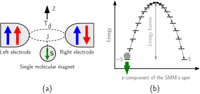
Figure 1: (color online)(a) Schematic picture of the system under consideration for two collinear configurations of the electrodes’ spin moments; parallel (blue arrows) and antiparallel (red arrows). Dashed lines represent the two possible tunneling processes: direct tunneling (the top line) and tunneling with scattering on the SMM’s spin due to exchange interaction (the bottom line). (b) Energy levels corresponding to different spin states of the SMM. The grey dot represents the initial spin state, $|-S\rangle$, of the molecule.

For the sake of simplicity we assume that the spin number $S$ of the molecule is constant, i.e. it does not change when current flows through the system. This also means that the charge state of SMM is fixed and only projection of the molecule’s spin on the quantization axis (anisotropy axis) can be changed due to the current. In addition, we restrict the following discussion to the case of weak coupling between the molecule and electrodes.

The full Hamiltonian of the system under consideration takes the form

$$\mathcal{H}=\mathcal{H}_{S\!M\!M}+\mathcal{H}_{L}+\mathcal{H}_{R}+\mathcal{H}_{T}.$$ (1)

The first term describes the SMM and is assumed in the form,

$$\mathcal{H}_{S\!M\!M}=-DS_{z}^{2},$$ (2)

where $S_{z}$ is the $z$ component of the spin operator, and $D$ is the uniaxial anisotropy constant. Although Eq. (2) represents the simplest Hamiltonian of a free SMM, it is sufficient for the effects to be described here. The next two terms describe ferromagnetic electrodes,

$$\mathcal{H}_{q}=\sum_{{\bf k}\alpha}\epsilon_{{\bf k}\alpha}^{q}\>a_{{\bf k}\alpha}^{q{\dagger}}a_{{\bf k}\alpha}^{q}$$ (3)

for $q=L$ (left lead) and $q=R$ (right lead). The electrodes are characterized by conduction bands with the energy dispersion $\epsilon_{{\bf k}\alpha}^{q}$, where ${\bf k}$ denotes a wave vector and $\alpha$ is the electron spin index. In Eq.(2) $a^{q}_{{\bf k}\alpha}$ and $a^{q{\dagger}}_{{\bf k}\alpha}$ are the relevant annihilation and creation operators, respectively.

The last term of the Hamiltonian $\mathcal{H}$ stands for the tunneling processes Appelbaum (1966, 1967); KimPRL04 ,

$$\mathcal{H}_{T}=\frac{1}{2}\sum_{q,q^{\prime}}\sum_{{\bf k}{\bf k}^{\prime}\alpha\beta}\frac{J_{q,q^{\prime}}}{\sqrt{N_{q}\,N_{q^{\prime}}}}\>\bm{\sigma}_{\alpha\beta}\cdot\mathbf{S}\>a_{{\bf k}\alpha}^{q{\dagger}}a_{{\bf k}^{\prime}\beta}^{q^{\prime}}\$$

$$+\sum_{{\bf k}{\bf k}^{\prime}\alpha}\frac{T_{d}}{\sqrt{N_{L}\,N_{R}}}\>a_{{\bf k}\alpha}^{L{\dagger}}a_{{\bf k}^{\prime}\alpha}^{R}\>+\>\textrm{H.c.}$$ (4)

The first term in the above equation describes tunneling with simultaneous interaction of tunneling electrons with the SMM via exchange coupling, with $J_{q,q^{\prime}}$ being the relevant exchange parameter. In a general case $J_{L,L}\neq J_{R,R}\neq J_{L,R}=J_{R,L}$. In the following, however, we assume symmetrical situation, where $J_{L,L}=J_{R,R}=J_{L,R}=J_{R,L}\equiv J$. The second term of Eq. (II) describes direct tunneling between the leads, with $T_{d}$ denoting the corresponding tunneling parameter. Apart from this, $\mathbf{S}$ is the SMM’s spin operator, and $\bm{\sigma}=(\sigma^{x},\sigma^{y},\sigma^{z})$ is the Pauli spin operator for conduction electrons. We assume that both, $T_{d}$ and $J$, are independent of energy and polarization of the leads. Additionally, $T_{d}$ and $J$ are normalized in such a way that they are independent of the size of electrodes, with $N_{q}$ ($q=L,R$) denoting the number of elementary cells in the $q$-th electrode.

The electric current flowing in the system is determined from the Fermi golden rule, KimPRL04 ,

$$I =e\sum_{mm^{\prime}}\sum_{{\bf k}{\bf k}^{\prime}\alpha\beta}\Bigg{\{}P_{m}\>W^{L{\bf k}\alpha m}_{R{\bf k}^{\prime}\beta m^{\prime}}\>f(\epsilon_{{\bf k}\alpha}^{L})\left[1-f(\epsilon_{{\bf k}^{\prime}\beta}^{R})\right]$$

$$\hskip 68.28644pt-(L{\bf k}\alpha m\leftrightarrow R{\bf k}^{\prime}\beta m^{\prime})\Bigg{\}},$$ (5)

where $e$ is the electron charge (for simplicity we assume $e>0$, so current is positive when electrons flow from left to right), $f(\epsilon)$ is the Fermi–Dirac distribution, $P_{m}$ is the probability to find the SMM in the spin state $|m\rangle$, and $W^{L{\bf k}\alpha m}_{R{\bf k}^{\prime}\beta m^{\prime}}$ is the rate of electron transitions from the initial state $\{L{\bf k}\alpha m\}$ to the final one $\{R{\bf k}^{\prime}\beta m^{\prime}\}$.

Up to the leading terms with respect to the coupling constants $T_{d}$ and $J$, the current is given by the formula

$$I =\frac{2\pi}{\hbar}\>e^{2}\>\Big{[}|T_{d}|^{2}+|J|^{2}\left\langle S_{z}^{2}\right\rangle\Big{]}\Big{(}D_{\uparrow}^{L}D_{\uparrow}^{R}+D_{\downarrow}^{L}D_{\downarrow}^{R}\Big{)}\>V\allowdisplaybreaks[1]$$

$$+\frac{2\pi}{\hbar}\>e\>|J|^{2}\>\sum_{m}P_{m}\sum_{\eta=+,-}\eta$$

$$\hskip 11.38092pt\times\Bigg{\{}D_{\downarrow}^{L}D_{\uparrow}^{R}A_{-\eta}(m)\zeta\Big{(}D(-\eta 2m+1)+\eta eV\Big{)}$$

$$\hskip 19.91684pt+D_{\uparrow}^{L}D_{\downarrow}^{R}A_{\eta}(m)\zeta\Big{(}D(\eta 2m+1)+\eta eV\Big{)}\Bigg{\}}.$$ (6)

Here, $D_{\sigma}^{q}$ is the density of states (DOS) at the Fermi level in the $q$-th electrode for spin $\sigma$, $\left\langle S_{z}^{2}\right\rangle=\sum_{m}m^{2}P_{m}$, and $V$ is the voltage between the leads, $eV=\mu_{L}-\mu_{R}$, with $\mu_{L}$ and $\mu_{R}$ denoting the electrochemical potentials of the leads. Finally, $A_{\pm}(m)=S(S+1)-m(m\pm 1)$, and $\zeta(\epsilon)=\epsilon\big{[}1-\exp(-\epsilon\beta)\big{]}^{-1}$ with $\beta^{-1}=k_{B}T$.

III Theoretical analysis

To calculate electric current from Eq. (II) we need to know the probabilities $P_{m}$. To find them, we assume the initial state of the SMM’s spin to be $|-S\rangle$, as indicated in Fig. 1(b). By applying a sufficiently large voltage, one can switch the molecule to the final state $|S\rangle$. The reversal process takes place via the consecutive intermediate states; $|-S+1\rangle,\ldots,|S-1\rangle$. In the following we assume that the voltage applied to the system grows linearly in time, $V=c\,t$, where $c$ denotes the velocity at which the voltage is increased. This allows to observe switching directly in the current flowing through the system when the voltage surpasses a critical value. The probabilities $P_{m}$ can be then found from the following master equations:

$$\left\{\begin{aligned} c\,\dot{P}_{S}\>=\>&-\>\gamma_{S}^{-}P_{S}\>+\>\gamma_{S-1}^{+}P_{S-1},\\ c\,\dot{P}_{m}\>=\>&-\>\gamma_{m}^{-}P_{m}\>-\>\gamma_{m}^{+}P_{m}\\ &+\>\gamma_{m+1}^{-}P_{m+1}\>+\>\gamma_{m-1}^{+}P_{m-1},\\ c\,\dot{P}_{-S}\>=\>&-\gamma_{-S}^{+}P_{-S}\>+\>\gamma_{-S+1}^{-}P_{-S+1},\end{aligned}\right.$$ (7)

for $-S<m<S$ and $\dot{P}$ defined as $\dot{P}\equiv dP/dV$. The transition rates $\gamma_{m}^{+(-)}$ are given by

$$\gamma_{m}^{+(-)} =\frac{2\pi}{\hbar}|J|^{2}A_{\pm}(m)$$

$$\hskip 11.38092pt\times\Big{\{}D_{\uparrow}^{L}D_{\downarrow}^{R}\zeta\Big{(}D(\pm 2m+1)\pm eV\Big{)}$$

$$\hskip 18.49411pt+D_{\downarrow}^{L}D_{\uparrow}^{R}\zeta\Big{(}D(\pm 2m+1)\mp eV\Big{)}$$

$$\hskip 18.49411pt+\Big{[}D_{\uparrow}^{L}D_{\downarrow}^{L}+D_{\uparrow}^{R}D_{\downarrow}^{R}\Big{]}\zeta\Big{(}D(\pm 2m+1)\Big{)}\Big{\}}.$$ (8)

The relevant boundary conditions are: $P_{-S}(V=0)=1$ and $P_{m}(V=0)=0$, for $m\neq-S$.

IV Numerical results and discussion

Numerical calculations have been performed for an octanuclear iron(III) oxo-hydroxo cluster of the formula $\left[\textrm{Fe}_{8}\textrm{O}_{2}(\textrm{OH})_{12}(\textrm{tacn})_{6}\right]^{8+}$ (shortly $\textrm{Fe}_{8}$), whose total spin number is $S=10$. The anizotropy constant is $D=0.292$ K Wernsdorfer and Sessoli (1999), and we assume that $J\approx T_{d}\approx 100$ meV. Furthermore, both the leads are assumed to be made of the same metallic material, with the elementary cells occupied by 2 atoms contributing 2 electrons each. The density of free electrons is assumed to be $n\approx 10^{29}m^{-3}$. The electrodes are characterized by the polarization parameter $P^{q}=(D_{+}^{q}\>-\>D_{-}^{q})/(D_{+}^{q}\>+\>D_{-}^{q})$, where $D_{+(-)}^{q}$ denotes the DOS of majority (minority) electrons in the $q$-th electrode. The temperature of the system is assumed to be $T=0.01$ K, which is below the blocking temperature $T_{B}=0.36$ K of $\textrm{Fe}_{8}$.

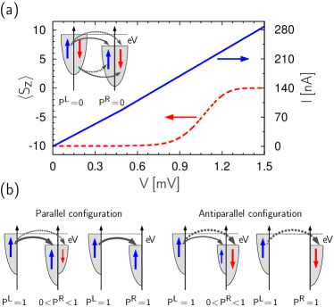
Figure 2: (color online) (a) The mean value of the SMM’s spin $\left\langle S_{z}\right\rangle$ and the current $I$ flowing through the system as a function of voltage $V$ in the case of nonmagnetic electrodes, and for $c=10$ kV/s and $T=0.01$ K. The inset shows schematically the density of states and the allowed tunneling processes (the solid arrows correspond to electrons tunneling without spin reversal, whereas the dashed arrows correspond to electrons tunneling with simultaneous spin-flip). (b) Schematic representation of the DOS and tunneling processes for both parallel and antiparallel magnetic configurations, shown in the case when the left electrode is made of a half-metallic ferromagnet while the right one is either a typical 3d ferromagnet or a half-metallic ferromagnet.

Let us begin with the case where both electrodes are nonmagnetic. In Fig. 2(a) we show the average value of the $z$ component of the SMM’s spin, $\langle S_{z}\rangle\>=\>\sum_{n=-S}^{S}nP_{n}$, and the charge current $I$. The spin reversal is not found, though the current affects the SMM’s spin for $V$ exceeding the threshold voltage determined by the anisotropy constant $D$ (energy level separation). At this voltage, transport associated with spin-flip of the conduction electrons becomes energetically allowed, exciting the molecule to the spin state $|-S+1\rangle$. As the voltage is increased further, the different SMM’s spin states $|m\rangle$ become equally probable and $\left\langle S_{z}\right\rangle\to 0$.

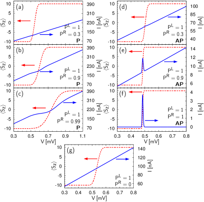
Figure 3: (color online) The mean value of the SMM’s spin $\left\langle S_{z}\right\rangle$ and the current $I$ flowing through the system as a function of voltage V for indicated polarization parameters in the parallel (P) (a)–(c) and antiparallel (AP) (d)–(f) configurations, and for $c=10$ kV/s and $T=0.01$ K. Part (g) corresponds to the case with one electrode being nonmagnetic.

The situation becomes significantly different when the electrodes are ferromagnetic, and tunneling processes are strongly spin dependent. The following discussion is limited to the most interesting situation, when one (say the left) electrode is a half-metallic ferromagnet with fully spin-polarized electrons at the Fermi level, $P^{L}=1$. The second electrode can be either nonmagnetic, or typical 3d ferromagnet, or even half-metallic. Tunneling processes with and without spin flip are indicated schematically in Fig.2(b). The corresponding transport characteristics and the average value of $S_{z}$ are shown in Fig. 3 for both parallel and antiparallel magnetic configurations of the leads, and for various spin polarizations of the right electrode. The complete reversal of the SMM’s spin becomes now possible, independently of the magnetic polarization of the right electrode. Starting with the spin state $|-S\rangle$ at zero bias, one arrives at the state $|S\rangle$ when the bias voltage surpasses the threshold value. Moreover, the switching leads to some features in the tunneling current. We note that switching also takes place for $0<P^{L}<1$, but the switching time becomes longer.

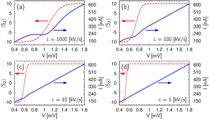
Figure 4: The mean value of the SMM’s spin $\left\langle S_{z}\right\rangle$ and the current $I$ as a function of the voltage $V$ for various voltage sweeping speeds $c$ in the parallel magnetic configuration of the system. The numerical results are for $T=0.01\>K$, $P^{L}=1$ and $P^{R}=0.9$.

In the parallel configuration, Figs 3(a)–(c), the reversal process can be observed as a dip in the current, which becomes more pronounced when $P^{R}\rightarrow 1$. The dip corresponds to the voltage range where the SMM’s spin reversal process takes place. It begins at the same voltage, $V\approx 0.48$ mV, which corresponds to the energy gap between the SMM’s spin states $|-S\rangle$ and $|-S+1\rangle$ (approximately $5.55$ K in the case considered). Because the energy gaps between the higher spin states are smaller, this energy is the activation energy for the current induced switching. Below the threshold voltage only direct tunneling (described by the second term in Eq.(4)) and the non-spin-flip part of the first term in Eq.(4) contribute to charge current. When the voltage activating spin reversal is reached, some of the tunneling electrons can flip their spins due to exchange interaction with the molecule, and this leads to spin reversal of the SMM. As a result $|\langle S_{z}\rangle|$ becomes reduced. This leads to partial suppression of the non-spin-flip contribution to current from the first term in Eq.(4). Instead of this, a spin-flip contribution becomes nonzero. However, the latter contribution is small as it involves DOS in the minority electron band of the right electrode, and cannot compensate the loss of current due to the non-spin-flip tunneling (which involves DOS for majority electrons). This leads effectively to a dip in the current, which occurs in the voltage range where spin switching of the SMM takes place. The dip disappears when spin of the SMM is completely reversed. The broadening of the dip, in turn, stems from the fact that as $P^{R}\rightarrow 1$, the transition times, $1/\gamma_{m}^{-(+)}$, become longer and longer (see Eq. (III)), and the time required for complete SMM’s spin reversal becomes longer as well. This also makes the dip more pronounced.

The situation is significantly different in the antiparallel configuration, Figs 3(d)–(f). Instead of the dip in current, there is now a peak in the voltage range where the switching takes place. This is because now the role of spin minority and spin majority electron bands in the right lead is interchanged. Additionally, the current flowing through the system tends to 0 when $P^{R}\rightarrow 1$ (perfect spin valve effect), except for a small voltage range where the reversal of the SMM’s spin occurs.

In the parallel configuration and for fully polarized electrodes ($P^{L}=P^{R}=1$), no reversal of the SMM’s spin occurs and a simple linear current-voltage characteristics is observed. On the other hand, the linear characteristics disappears in the antiparallel configuration, and the current does not flow through the system except for the voltage range where the magnetic switching of the molecule takes place, Fig. 3(f).

The probabilities $P_{m}$ depend on the velocity $c$ of the voltage increase, Eq. (7). In Fig.4 we show $\langle S_{z}\rangle$ and current $I$ in the parallel configuration and for several values of $c$. The magnetic switching becomes clearly visible as a dip in the current for larger values of $c$, Fig. 4(a). At smaller values of $c$, the reversal is not resolved in the current, Fig. 4(d). In fact, the change in $c$ does not affect the time range within which the magnetic switching takes place, but it only modifies the dependence between the time and voltage scales. As a result, the transition times $1/\gamma_{m}^{-(+)}$ become effectively longer within the time scale set by the rate at which the voltage is increased. Therefore for the higher speeds one can observe the broadening of the dip.

In summary, we showed that spin of a SMM can be reversed by a spin polarized current, and the switching process may be visible in current when voltage is increased in time. Full reversal of the molecule’s spin can be reached when at least one electrode is spin polarized. The numerical results presented above apply to the case with one electrode being fully spin polarized. However, the current-induced switching also takes place when spin polarization of this electrode is smaller. The switching time becomes then appropriately longer. Moreover, for the parameters assumed in numerical calculations the switching for positive current was only from the state $|-S\rangle$ to $|S\rangle$. If the molecule would be initially in the state $|S\rangle$, switching to the state $|-S\rangle$ could be achieved by negative (reversed) current.

Acknowledgements This work is supported by funds of the Polish Ministry of Science and Higher Education as a research project in years 2006-2009.

References

- Gatteschi and Sessoli (2003) D. Gatteschi and R. Sessoli, Angew. Chem. Int. Ed. 42, 268 (2003).
- Sessoli et al. (1993) R. Sessoli, D. Gatteschi, A. Caneschi, and M. A. Novak, Nature (London) 365, 141 (1993).
- Heersche et al. (2006) H. Heersche et al., Phys. Rev. Lett. 96, 206801 (2006).
- Jo et al. (2006) M.-H. Jo et al., Nano Lett. 6, 2014 (2006).
- Elste and Timm (2006) F. Elste and C. Timm, Phys. Rev. B 73, 235305 (2006).
- Romeike et al. (2006) C. Romeike, M. Wegewijs, and H. Schoeller, Phys. Rev. Lett. 96, 196805 (2006).
- Romeike et al. (2006) C. Romeike et al., Phys. Rev. Lett. 96, 196601 (2006).
- Timm and Elste (2006) C. Timm and F. Elste, Phys. Rev. B 73, 235304 (2006).
- (9) J. A. Katine, F.J. Albert, R.A. Buhrman, E.B. Myers, and D.C. Ralph, Phys. Rev. Lett. 84, 3149 (2000).
- (10) W. Rudziński and J. Barnaś, Phys. Rev. B 64, 085318 (2001).
- (11) J. Koenig, J. Martinek, J. Barnaś , and G. Schoen, in Lecture Notes in Physics 658, pp 145-164 (Springer-Verlag Berlin Heidelberg 2005) and references therin.
- (12) I. Weymann, J. Barnaś, Phys. Rev. B 73, 205309 (2006).
- (13) K. Hamaya, S. Masubuchi, M. Kawamura, T. Machida, M. Jung, K. Shibata, and K. Hirakawa, T. Taniyama, S. Ishida and Y. Arakawa, cond-mat/0611269 (unpublished).
- Appelbaum (1966) J. Appelbaum, Phys. Rev. Lett. 17, 91 (1966).
- Appelbaum (1967) J. Appelbaum, Phys. Rev. 154, 633 (1967).
- (16) G.-H. Kim and T.-S. Kim, Phys. Rev. Lett. 92, 137203 (2004).
- Wernsdorfer and Sessoli (1999) W. Wernsdorfer and R. Sessoli, Science 284, 133 (1999).