A unified origin for the 3D magnetism and superconductivity in Na_xCoO₂

Abstract

We analyze the origin of the three dimensional (3D) magnetism observed in nonhydrated Na-rich Na_xCoO₂ within an itinerant spin picture using a 3D Hubbard model. The origin is identified as the 3D nesting between the inner and outer portions of the Fermi surface, which arise due to the local minimum structure of the $a_{1g}$ band at the $\Gamma$-A line. The calculated spin wave dispersion strikingly resembles the neutron scattering result. We argue that this 3D magnetism and the spin fluctuations responsible for superconductivity in the hydrated systems share essentially the same origin.

The discovery of superconductivity (SC) in Na_xCoO${}_{2}\cdot y$ H₂O has attracted much attention.Takada Although the experiments are still somewhat controversial, we briefly summarize the present understanding. (i) Up to now, all the angle resolved photoemission (ARPES) measurements Hasan ; Yang2 ; Takeuchi ; Shimojima show the absence of the $e_{g}^{\prime}$ hole pockets predicted in the first principles calculation.Singh Thus the remaining $a_{1g}$ seems to be the relevant band. (ii) In the bilayer hydrated (BLH) SC samples, there is an enhancement in $(T_{1}T)^{-1}$ at low temperatures at the Co site Ishida3 ; Fujimoto ; Imai ; Ihara ; Michioka and at the O site, Imai ; Ihara2 ($T_{1}^{-1}$ is the spin-lattice relaxation rate) indicating the presence of spin fluctuations (SF) located away from the Brillouin zone (BZ) edge,Imai ; Ihara2 while such an enhancement is not seen in non-SC monolayer hydrated and nonhydrated Na-poor samples. On the other hand, the Knight shift stays nearly constant at low temperatures in the SC samples,Imai ; Ihara2 ; Alloul which means that the SF is not purely ferromagnetic. The bottom line is that SF that is neither purely ferromagnetic nor antiferromagnetic is strongly related to SC. (iii) Unconventional SC gap is suggested from the absence of the coherence peak in $T_{1}^{-1}$ as well as the power law decay below $T_{c}$.Ishida3 ; Fujimoto ; Kobayashi ; Zheng Several experiments suggest spin singlet pairing,Kobayashi ; Zheng2 and moreover, the effect of the impurities on $T_{c}$ is found to be small, Yokoi ; Oeschler suggesting a $s$-wave like gap.

In a previous paper, as a solution for understanding these experimental results, we have proposed a mechanism for an unconventional $s$-wave pairing, in which the local minimum structure (LMS) of the $a_{1g}$ band at the $\Gamma$ point plays an important role.Kuroki For appropriate band fillings, LMS results in disconnected inner and outer Fermi surfaces (FS), whose partial nesting induces SF at wave vectors that bridge the two FS (see Fig.6 left panel). This incommensurate SF can give rise to an “extended $s$-wave” pairing in which the gap changes sign between the two FS, but not within each FS. A recent multiorbital analysis also shows that such a pairing can occur when the inner and outer $a_{1g}$ FS are present.MO

The purpose of this paper is to investigate the relation between this SC and the 3D spin-density-wave(SDW)-like, metallic magnetism observed in the nonhydrated Na-rich systems, Motohashi ; Sugiyama ; Foo ; Keimer1 whose magnetic structure has been revealed by neutron scattering experiments to have in-plane ferromagnetic and out-of-plane antiferromagnetic character. Keimer2 ; Helme Neutron scattering experiments have further obtained the spin wave dispersion of this 3D magnetism. Analysis of this dispersion based on the localized spin picture have found that the out-of-plane antiferromagnetic coupling is of the order of the in-plane ferromagnetic coupling, Keimer2 ; Helme ; Johannes despite the strong 2D nature of the material. Moreover, Curie-Weiss temperature is expected to be positive from the evaluated coupling constants,Keimer2 while it is actually negative. Motohashi ; Sugiyama ; Foo ; Keimer1 ; Galivano ; Wang ; Alloul A theory based on a spin-orbital polaron picture has been proposed for this puzzle.Khaliullin

In the present study, since the system remains metallic in the magnetically ordered state, we take an itinerant spin viewpoint. From the consistency between the experiments and the calculated results, we propose that the origin of the 3D magnetism is essentially the same with the SF responsible for SC : the nesting between inner and outer portions of the Fermi surface that arises due to the local minimum of the $a_{1g}$ band.Korshunov

There exist two CoO₂ layers within a unit cell due to the alternation of the oxygen arrangement, but neither the effective hopping integrals nor the on-site energy alter along the $c$ axis, so the BZ folding in the $c$ direction occurs without inducing a gap in the band. Thus, in a 3D effective theory in which O and Na site degrees of freedom are integrated out, the unit cell contains only one layer, which results in an unfolded BZ shown in the upper right of Fig.1. Taking into account only the $a_{1g}$ band, we consider a single band Hubbard model $H=\sum_{i,j}\sum_{\sigma}t_{ij}c_{i\sigma}^{\dagger}c_{j\sigma}+U\sum_{i}n_{i\uparrow}n_{i\downarrow}$, on a 3D triangular lattice, where the 1st, 2nd and 3rd neighbor in-plane hopping integrals $t_{1}$, $t_{2}$, $t_{3}$ and the out-of-plane nearest neighbor hopping $t_{z}$ (Fig.1 upper left) are chosen so as to roughly reproduce the $a_{1g}$ portions of the band obtained in the first principles calculation.Singh Throughout the paper, we take $t_{2}=-0.35$, $t_{3}=-0.07$, and $t_{z}=-0.15$ (unless otherwise noted) in units of $t_{1}=1$, which corresponds to about (or slightly less than) 0.1eV according to ARPES measurements.Takeuchi The band (with $U=0$) for this choice of parameter values is shown in Fig.1. The band filling is $n=$number of electrons/site, and it is related to the actual Na content $x$ by $n-1=x$ (provided that the $e_{g}^{\prime}$ bands are fully occupied). We calculate the spin susceptibility using the fluctuation exchange (FLEX) approximationBickers as $\chi_{s}(q)=\chi_{\rm irr}(q)/[1-U\chi_{\rm irr}(q)]$, where $q=(\mbox{\boldmath$q$},i\omega_{n})$. Here, the irreducible susceptibility is $\chi_{\rm irr}(q)=-\frac{1}{N}\sum_{k}G(k+q)G(k)$ ($N$:number of $k$-point meshes), where $G$ is the renormalized Green’s function self-consistently obtained from the Dyson’s equation, in which the self energy is calculated using $G$ and $\chi_{\rm irr}$. We take up to $N=64\times 64\times 64$ $k$-point meshes and up to 16384 Matsubara frequencies.

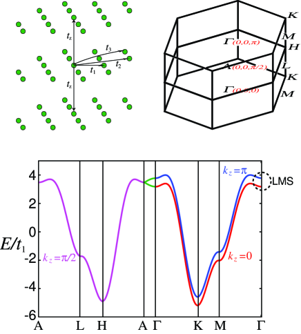
Figure 1: (color online) Upper left: the 3D model in the present study. Upper right: the Brillouin zone. The wave numbers in the parenthesis are those in the unfolded BZ scheme. Lower panel: the band structure of the present model with $U=0$. $k_{z}=0,\pi/2,\pi$ are $k_{z}$ in the unfolded BZ scheme.

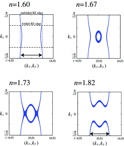
Figure 2: (color online) The vertical cross section $(k_{y}=0)$ of the FS for various $n$ with $U=0$. Here we use the unfolded BZ scheme, but for $n=1.60$ we also show the FS in the usual folded BZ scheme by dashed lines. The unfolded BZ edge in the $k_{z}$ direction is denoted as “$\frac{\pi}{c/2}$” to stress that the unit cell is halved in the $c$ direction. The finite thickness is due to a finite range of energy $(E_{F}\pm 0.03t_{1})$ taken in obtaining the FS. The thickness thus represents the density of states or the effective mass. The arrows present the diameter of the FS.

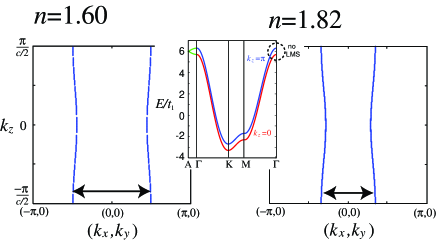
Figure 3: (color online) Similar as in Fig.2 except $t_{2}=t_{3}=0$. The band is shown in the inset.

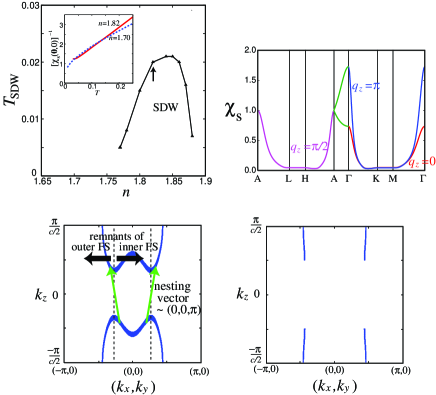
Figure 4: (color online) Upper left: The band filling dependence of $T_{\rm SDW}$ obtained by FLEX. The inset shows the $T$ dependence of $\chi_{s}(\mbox{\boldmath$0$},0)^{-1}$ for $n=1.82$ and $n=1.7$. Upper right: The FLEX $\chi_{s}(\mbox{\boldmath$q$},0)$ for $n=1.82$, $U=6$, and $T=0.05$. Lower left: the nesting vector of the FS for $n=1.82$ is shown. Lower right: The FS in the ordered state $(T=0.015)$ obtained by the mean field calculation is shown. Although the unit cell is “truely” doubled in this case ($\pi/2<|k_{z}|<\pi$ part should actually be drawn repeatedly in $0<|k_{z}|<\pi/2$ region), we continue to use the unfolded scheme for a clear comparison with the FS in the non-ordered state in the left.

In order to analyze the magnetically ordered state with a wave vector $Q$ at which the FLEX spin susceptibility is maximized, we consider a mean field Hamiltonian

$$H=\sum_{\sigma=\uparrow,\downarrow}\sum_{\mbox{\boldmath$k$}}\sum_{m=0,1}\left[\varepsilon(\mbox{\boldmath$k$}+m\mbox{\boldmath$Q$})c^{\dagger}_{\mbox{\boldmath$k$}+m\mbox{\boldmath$Q$},\sigma}c_{\mbox{\boldmath$k$}+m\mbox{\boldmath$Q$},\sigma}\right.$$

$$\left.+U\sum_{l=0,1}\langle n_{m\mbox{\boldmath$Q$},-\sigma}\rangle c^{\dagger}_{\mbox{\boldmath$k$}+(m+l)\mbox{\boldmath$Q$},\sigma}c_{\mbox{\boldmath$k$}+m\mbox{\boldmath$Q$},\sigma}\right]$$

$$=\sum_{\sigma=\uparrow,\downarrow}\sum_{\mbox{\boldmath$k$}}\sum_{\alpha=1,2}E_{\alpha,\sigma}(\mbox{\boldmath$k$})\gamma^{\dagger}_{\mbox{\boldmath$k$},\sigma,\alpha}\gamma_{\mbox{\boldmath$k$},\sigma,\alpha}$$

where $\varepsilon({\mbox{\boldmath$k$}})$ is the bare band dispersion, $c_{\mbox{\boldmath$k$}+m\mbox{\boldmath$Q$},\sigma}=\sum_{\alpha=1,2}u_{\alpha,\sigma,m}(\mbox{\boldmath$k$})\gamma_{\mbox{\boldmath$k$},\sigma,\alpha}$ is a unitary transformation that diagonalizes the Hamiltonian to obtain the two bands $E_{1\sigma}$ and $E_{2\sigma}$, and $\langle n_{\mbox{\boldmath$Q$},\sigma}\rangle$ is self-consistently determined in the usual procedure. We then calculate the irreducible susceptibility matrix by

$$\left(\chi_{0}^{\sigma\sigma^{\prime}}(\mbox{\boldmath$k$},\omega)\right)_{ij}=\frac{1}{N}\sum_{\mbox{\boldmath$p$}}\sum_{m,n,\alpha,\alpha^{\prime}}u_{\alpha,\sigma,m+i}(\mbox{\boldmath$p$}+\mbox{\boldmath$k$})$$

$$\times u_{\alpha,\sigma,m+n+j}(\mbox{\boldmath$p$}+\mbox{\boldmath$k$})u_{\alpha^{\prime},\sigma^{\prime},m+n}(\mbox{\boldmath$p$})u_{\alpha^{\prime},\sigma^{\prime},m}(\mbox{\boldmath$p$})$$

$$\times\frac{f(E_{\alpha^{\prime},\sigma^{\prime}}(\mbox{\boldmath$p$}))-f(E_{\alpha,\sigma}(\mbox{\boldmath$p$}+\mbox{\boldmath$k$}))}{E_{\alpha,\sigma}(\mbox{\boldmath$k$}+\mbox{\boldmath$p$})-E_{\alpha^{\prime},\sigma^{\prime}}(\mbox{\boldmath$p$})+\omega+i\epsilon},$$

where $f(E)$ is the Fermi distribution function. The spin wave dispersion can be determined by the condition that the real part of the eigenvalue of the matrix $1-U\chi^{\uparrow\downarrow}_{0}(\mbox{\boldmath$q$},\omega)$ equals zero. We take up to $N=192\times 192\times 96$ $k$-point meshes here.

We first show in Fig.2 the evolution of the 3D FS (with $U=0$) as the band filling is increased. Here the vertical cross section of the FS is given in the unfolded BZ. The FS is a 2D cylinder for small band filling, that is, for low Na content. As the band filling is increased, an inner FS appears around the $\Gamma$ point. As in the purely 2D($\sim$ BLH) case (see Fig.6 or ref.Kuroki, ), this FS is disconnected from the outer 2D cylindrical FS, but the inner FS is 3D in the NH case.comment5 For larger band fillings, the two FS become connected (around $n=1.73$), and then finally for higher band fillings it becomes a single 3D FS. The appearance of the 3D FS despite the small $t_{z}$ is a consequence of LMS of the band along the $\Gamma$-A line. In fact, if we take a band that does not have LMS, $i.e.,$ for $t_{2}=t_{3}=0$ but with the same $t_{z}(=-0.15)$, the FS remains to be 2D (unless the band filling becomes very close to 2) as shown in Fig.3. The 3D evolution of the FS is consistent with the ARPES observations, where the in-plane $k_{F}$ barely decreases with the increase of the Na content for $x>0.6$.Yang2 ; Hasan2 In fact, the decrease of the FS diameter in Fig.2 is very small compared to that in Fig.3.

In the inset of the upper left of Fig.4 , FLEX results of $\chi^{-1}_{s}(\mbox{\boldmath$q$}=0,i\omega_{n}=0)$ are plotted as functions of $T$ for $U=6$ and $n=1.82$ or $n=1.7$. The Curie-Weiss behavior at high temperatures with a negative Curie-Weiss temperature is consistent with the experiments. Motohashi ; Sugiyama ; Galivano ; Keimer1 ; Foo ; Wang ; Imai ; Alloul In the upper left of Fig.4, $T_{\rm SDW}$, defined as the temperature where the maximum value of $U\chi_{\rm irr}$ reaches $\simeq 1$, is plotted as a function of the band filling. $T_{\rm SDW}$ exists only in the regime $1.75<n<1.9$, which is consistent with the fact that the magnetic ordering is not observed experimentally for $x<0.75$.Foo ; Imai The maximum $T_{\rm SDW}$ corresponds to about 20K, in agreement with the experiments.Motohashi ; Sugiyama ; Keimer1 Around $n\sim 1.8$, the ordering occurs with $\mbox{\boldmath$Q$}=(0,0,\pi)$, as shown in the upper right of Fig.4 for $n=1.82$, which corresponds to in-plane ferromagnetic, out-of-plane antiferromagnetic spin structure, as found experimentally.Keimer2 ; Helme The origin of this spin correlation can be found in the shape of the 3D FS. Namely, the FS at $n\sim 1.8$ is partially nested with a nesting vector close to $(0,0,\pi)$, as can be seen in Fig.4 (lower left panel). In fact, this nesting occurs between portions of the FS that can be considered as remnants of the inner and outer FS, which are disconnected for lower band fillings.comment2 On the other hand, as the band filling comes close to $n=1.9$ ($x=0.9$), the FS becomes too small for $(0,0,\pi)$ nesting, and the ordering wave number becomes incommensurate in the $c$ direction, which is also consistent with the finding in ref.Sugiyama, .

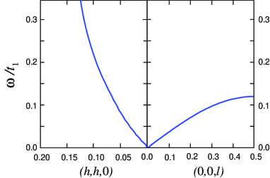
Figure 5: (color online) The calculated in-plane (left) and out-of-plane (right) spin wave dispersion for $n=1.82$, $U=4$, and $T=0.015$. Here the wave vectors are presented in units of the reciprocal lattice primitive vector in the usual folded BZ for clear comparison with Fig.4 of ref.Keimer2, .

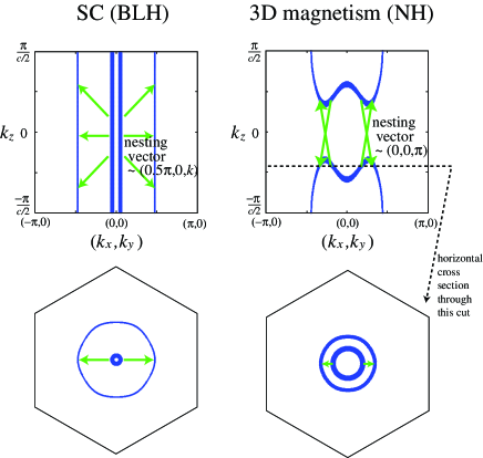
Figure 6: (color online) The FS nesting relevant for SC and the 3D magnetism.

We now move on to the mean field results in the $\mbox{\boldmath$Q$}=(0,0,\pi)$ SDW ordered state. We focus on $n=1.82$ and take $U$ smaller than $U=6$ adopted in FLEX since the mean field approach tends to overestimate the tendency toward ordering. In fact, taking $U=4$ gives a self-consistently determined $\langle n_{\mbox{\boldmath$Q$}\uparrow}\rangle$ value of 0.075 at low $T$, corresponding to a magnetic moment of $0.15\mu_{B}$ per site (Co atom), in rough agreement with a $\mu$SR estimation $0.18\mu_{B}$.Sugiyama In Fig.4 (lower right panel), we show the calculation result of the FS in the ordered state. The portions of the FS around $k_{z}=\pm\pi/2$ disappear, but other portions remain to result in a FS with a strong 2D character. This is consistent with the fact that system remains metallic in the magnetically ordered state.Motohashi Note also that the disappearing portions of the FS are thick, i.e., they have heavy mass, which is consistent with what has been suggested in ref.Motohashi, from the enhancement of the mobility in the magnetically ordered state.

In Fig.5, we show the calculated spin wave dispersion. The overall feature as well as the in-plane to out-of-plane ratio $\omega(0.1,0.1,0)/\omega(0,0,0.5)\sim 2.1$ strikingly resembles the neutron scattering result of ref.Keimer2, for $x=0.82$. The energy scale ($\omega(0,0,0.5)\simeq 0.1t_{1}$ corresponds to $\sim 10$ meV) is also close to the experimental result. Here again, our results show that the 3D magnetism is well understood within the present itinerant spin picture.Sushko

Finally, let us discuss the relation between this 3D magnetism and SC. As we have seen, the SF in the nonhydrated systems becomes weak for small band fillings. This is because the nesting between the 2D outer and the 3D inner FS is not good. However, the nesting between the inner and the outer FScomment3 can be restrengthened if the two dimensionality is increased by hydration, resulting in enhanced SF. As we have mentioned in the beginning, our proposal is that this SF is responsible for SC.Kuroki Thus, in our view, the 3D magnetism and the incommensurate SF that gives rise to SC share the same origin as shown in Fig.6: the nesting between the inner and the outer (connected or disconnected) FS that originate from the local minimum of the $a_{1g}$ band.

Numerical calculation were performed at the facilities of the Supercomputer Center, ISSP, University of Tokyo. This study has been supported by Grants-in-Aid for Scientific Research from the Ministry of Education, Culture, Sports, Science and Technology of Japan, and from the Japan Society for the Promotion of Science.

References

- (1) Present affiliation: NHK Spring Co.
- (2) Present affiliation: Nikon Co.
- (3) K. Takada et al., Nature 422, 53 (2003).
- (4) M.Z. Hasan et al., Phys. Rev. Lett. 92, 246402 (2004).
- (5) H.-B. Yang et al., Phys. Rev. Lett. 95, 146401 (2005).
- (6) T. Takeuchi et al., Proc. 24th Int. Conf. Thermoelectrics. (2005) p.435.
- (7) T. Shimojima et al., cond-mat/0606424.
- (8) D.J.Singh, Phys. Rev. B 61, 13397 (2000).
- (9) K. Ishida et al., J. Phys. Soc. Jpn. 72, 3041 (2003).
- (10) T. Fujimoto et al., Phys. Rev. Lett. 92, 047004 (2004).
- (11) F.L. Ning et al., Phys. Rev. Lett. 93, 237201 (2004); F.L. Ning and T. Imai, Phys. Rev. Lett. 94, 227004 (2005).
- (12) Y. Ihara et al., J. Phys. Soc. Jpn. 74, 867 (2005).
- (13) C. Michioka et al., J. Phys. Soc. Jpn. 75, 063701 (2006).
- (14) Y. Ihara et al., J. Phys. Soc. Jpn. 74, 2177 (2005).
- (15) I.R. Mukhamedshin et al., Phys. Rev. Lett. 94, 247602 (2005).
- (16) Y. Kobayashi et al., J. Phys. Soc. Jpn. 74, 1800 (2005).
- (17) G.-q. Zheng et al., J. Cond. Matt. 18, L63 (2006).
- (18) G.-q. Zheng et al., Phys. Rev. B 73, 180503 (2006).
- (19) M. Yokoi et al., J. Phys. Soc. Jpn. 73, 1297 (2004).
- (20) N. Oeschler et al., cond-mat/0503690.
- (21) K. Kuroki et al., Phys. Rev. B 75, 051013 (2006).
- (22) M. Mochizuki and M. Ogata, cond-mat/0609443, to be published in J. Phys. Soc. Jpn.
- (23) T. Motohashi et al., Phys. Rev. B 67, 064406 (2003).
- (24) J. Sugiyama et al., Phys. Rev. B 67, 214420 (2003); ibid. 69 214423 (2004).
- (25) M.L. Foo et al., Phys. Rev. Lett. 92, 247001 (2004).
- (26) S.P. Bayrakci et al., Phys. Rev. B 69, 100410 (2004).
- (27) S.P. Bayrakci et al., Phys. Rev. Lett. 94, 157205 (2005).
- (28) A.T.Boothroyd et al, Phys. Rev. Lett. 92, 197201 (2004); L.M. Helme et al., Phys. Rev. Lett. 94, 157206 (2005).
- (29) M.D. Johannes et al., Phys. Rev. B 71, 214410 (2005).
- (30) J.L. Galivano et al., Phys. Rev. B 69, 100404 (2004).
- (31) Y. Wang et al., Nature 423, 425 (2003).
- (32) M. Daghofer et al., Phys. Rev. Lett. 96, 216404 (2006).
- (33) Quite recently, M.M. Korshunov et al. in cond-mat/0608327 discuss the relation between LMS and ferromagnetic SF, but neglect the three dimensionality of the system.
- (34) N.E. Bickers, D.J. Scalapino, and S.R. White, Phys. Rev. Lett. 62, 961 (1989).
- (35) The term “inner” and “outer” FS in the present study should not be mixed up with the commonly known “bilayer-coupling-originated inner and outer” FS, which in the unfolded BZ scheme correspond to FS at and (see Fig.2, ).
- (36) D. Qian et al., Phys. Rev. Lett. 96, 216405 (2006).
- (37) We have investigated other sets of hopping values and found that the spin correlation (with a possible slight incommensurability as expected from the nesting vector) is robust when the band filling is around as far as LMS of the band exists.
- (38) In cond-mat/0509308, Y.V. Sushko et al. find that the magnetic ordering temperature increases with applying pressure, unusual for an SDW state. In fact, applying pressure should increase , which according to our FLEX calculation favors the SDW (as far as the increase of is within ) because the origin of the nesting here is the 3D FS itself. Applying pressure may also increase and , which makes LMS of the band deeper, and thus also favors the SDW.
- (39) The inner FS can appear despite the low Na content of because of the presence of H3O+ ions suggested in e.g., H. Sakurai et al., Phys. Rev. B 74, 092502 (2006).