Stress-free states of continuum dislocation fields: Rotations, grain boundaries, and the Nye dislocation density tensor

Abstract

We derive general relations between grain boundaries, rotational deformations, and stress-free states for the mesoscale continuum Nye dislocation density tensor. Dislocations generally are associated with long-range stress fields. We provide the general form for dislocation density fields whose stress fields vanish. We explain that a grain boundary (a dislocation wall satisfying Frank’s formula) has vanishing stress in the continuum limit. We show that the general stress-free state can be written explicitly as a (perhaps continuous) superposition of flat Frank walls. We show that the stress-free states are also naturally interpreted as configurations generated by a general spatially-dependent rotational deformation. Finally, we propose a least-squares definition for the spatially-dependent rotation field of a general (stressful) dislocation density field.

I Introduction

The crystalline phase breaks two continuous symmetries: translational invariance and rotational invariance. Dislocations are the topological defect associated with broken translational symmetry. Rotational distortions in crystals relax into wall structures formed from arrays of dislocations. It would seem natural to describe the formation and evolution of these mesoscale dislocation structures using a continuum dislocation density theory. Individual dislocations are associated with long-range stress fields, and the dislocation evolution and structure formation is strongly constrained by the need to screen these stresses. In the 1950s, a number of authors Eshelby (1956); Kröner (1958, 1981); Kosevich (1962); Mura (1963, 1991) (building on ideas from differential geometry) developed such a continuum description involving the coarse-grained net topological charge of the dislocations in a region, organized into dislocation density tensor named for Nye. Since the long-range stress fields and the rotational distortions only depend upon the net dislocation density, it is natural for us to use this order parameter to describe the connections between rotations, dislocations, and stress. In this manuscript, we provide a systematic mathematical analysis of the relations between rotational deformations, domain walls, and dislocation stress within the framework of Nye’s continuum dislocation density tensor.

In equilibrium, a large crystal with boundary conditions imposing a rotational deformation will relax by forming a few grain boundaries—sharp walls formed by dislocation arrays, separating perfect crystalline grains, with elastic stress confined locally near the grain boundaries. In the continuum theory, the region of local elastic stress vanishes, and grain boundaries are described as $\delta$-function dislocation densities with zero stress. We analyze stress-free dislocation walls in the continuum theory in section III, and connect them with Frank’s formula Frank (1950) for the dislocation content of grain boundaries in appendix A.

At high temperatures, an initially disordered or microscopically deformed material will approach equilibrium through the formation and coarsening of polycrystals—the rotation gradients are confined to sharp grain boundaries, separating local regions of different orientations. Again, the strain fields in a polycrystal are confined to small regions around the grain boundaries. In the continuum dislocation theory a polycrystal is thus a stress-free configuration of dislocations. In section II, we derive the most general solution for the dislocation density tensor with zero stress. In section III, we show that this solution can be decomposed into a superposition of flat grain boundaries. In appendix B and figure 3 we explicitly represent a (zero-stress) curved grain boundary as a continuum superposition of flat walls. In section IV, we also show that the most general stress-free state can be represented in terms of a local rotation field. Hence the stress-free states in the continuum theory can be interpreted as polycrystals with arbitrarily small crystallites; the strain energy for grain boundaries is zero, so the crystalline axes can vary arbitrarily in space. This would suggest that sharp, discrete wall formation is not implied by the energetics within the continuum theory; recent work elsewhere Limkumnerd and Sethna (2006a, b) has shown that they may nonetheless form via shock formation in the natural dislocation dynamics.

At low temperatures, where mass transport by diffusion of vacancies and interstitial diffusion is frozen out, external strain is relieved by (volume-preserving) dislocation glide. The motion, entanglement, and multiplication of dislocations under this low-temperature plastic deformation leads to work hardening and the development of a yield stress. These systems have long been modeled using continuum dislocation theories,Limkumnerd and Sethna (2006a, b); Groma (1997); Bakó and Groma (1999); Zaiser et al. (2001); El-Azab (2000); Roy and Acharya (2005); Acharya and Sawant (2006); Acharya and Roy (2006); Roy and Acharya (2006) sometimes simplifying the dislocation density into a scalar quantity, but sometimes incorporating information not contained in the Nye tensor (‘geometrically unnecessary’ dislocation densities with canceling topological charge, yield stress laws, and separate dislocation densities for each slip system, …). Continuum dislocation theories have been important not only in understanding large-scale discrete dislocation simulations,Miguel et al. (2001a); Bakó and Groma (1999); Barts and Carlsson (1997); Gullouglu and Hartly (1993); Groma and Pawley (1993a, b); Fournet and Salazar (1996); Benzerga et al. (2004, 2005); Groma and Bakó (2000); Gómez-García et al. (2006) but also in understanding emergent dislocation avalanche phenomena.Zaiser et al. (2001); Miguel et al. (2001a, b, 2002); Weiss and Marsan (2003); Richeton et al. (2005); Sammonds (2005); Miguel and Zapperi (2006); Zaiser (2006); Dimiduk et al. (2006) At large deformations (stage III plasticity), these tangles of dislocations begin to organize again into walls (here called cell walls) separating largely undeformed regionsHughes et al. (1998); Kuhlmann-Wilsdorf and Hansen (1991); Hughes and Hansen (1993, 1995, 2001); Hughes (2001) with small misorientation angles between cells (again potentially explained by a shock formation in the climb-free dynamical evolution law Limkumnerd and Sethna (2006a, b)). In section V we provide the relation between the local rotation field for a general dislocation density tensor, which (for general stressful densities) is a formula providing a least-squares best approximation for the local orientation of the crystalline axes.

II The general stress-free dislocation density

A dislocation is a crystallographic defect representing extra rows or columns of atoms and is characterized by two quantities; its line direction $\mathbf{t}$, and its Burgers vector $\mathbf{b}$. After a passage around a closed contour $C$ that encircles a dislocation line, a displacement field $\mathbf{u}$ receives an increment $\mathbf{b}$ according to

$$\oint_{C}du_{i}=\oint_{C}\beta^{\text{P}}_{ij}\,dx_{j}=-b_{i}$$ (1)

where $\bm{\beta^{\text{P}}}$ describes the irreversible plastic deformation. The Nye dislocation density tensor $\bm{\rho}$ is defined by $\bm{\rho}=(\mathbf{t}\otimes\mathbf{b})\delta(\bm{\xi})$ where $\bm{\xi}$ is the two-dimensional radius vector measured from the axis of the dislocation in the plane locally perpendicular to $\mathbf{t}$. When many dislocations labeled by $\alpha$ are present, a coarse-graining description of a conglomerate of dislocations is preferred. In this picture,

$$\rho_{ij}(\mathbf{x})=\sum_{\alpha}\int t^{\alpha}_{i}b^{\alpha}_{j}\delta(\mathbf{x}^{\prime}-\bm{\xi}^{\alpha})G(\mathbf{x}-\mathbf{x}^{\prime})d^{3}\mathbf{x}^{\prime},$$ (2)

with Gaussian weighting $G(\mathbf{x}-\mathbf{x}^{\prime})\simeq(1/\sqrt{2\pi}L)^{3}\,\text{exp}[-(\mathbf{x}-\mathbf{x}^{\prime})^{2}/(2L^{2})]$ over some distance scale $L$ large compared to the distance between dislocations and small compared to the dislocation structures being modeled. Since dislocation lines are topological and cannot end inside the crystal, $\bm{\rho}$ is divergence free: $\partial_{i}\rho_{ij}=0$.

A dislocation strains the crystal, and creates a long-range stress field. Peach and Koehler derived the relationship for stress fields due to dislocations in an isotropic material.Peach and Koehler (1950) In terms of the Nye dislocation tensor $\bm{\rho}$, the stress can be written as the sum of two convolutions:

$$\sigma_{\alpha\beta}(\mathbf{x})=-\frac{\mu}{8\pi}\int_{V}\\ \Big{[}(\varepsilon_{im\alpha}\rho_{\beta m}(\mathbf{x}^{\prime})+\varepsilon_{im\beta}\rho_{\alpha m}(\mathbf{x}^{\prime}))\frac{\partial^{3}|\mathbf{x}-\mathbf{x}^{\prime}|}{\partial x^{\prime}_{i}\partial x^{\prime}_{j}\partial x^{\prime}_{j}}-\frac{\mu}{4\pi(1-\nu)}\\ \varepsilon_{imk}\rho_{km}(\mathbf{x}^{\prime})\left(\frac{\partial^{3}|\mathbf{x}-\mathbf{x}^{\prime}|}{\partial x^{\prime}_{i}\partial x^{\prime}_{\alpha}\partial x^{\prime}_{\beta}}-\delta_{\alpha\beta}\frac{\partial^{3}|\mathbf{x}-\mathbf{x}^{\prime}|}{\partial x^{\prime}_{i}\partial x^{\prime}_{j}\partial x^{\prime}_{j}}\right)\Big{]}\,d^{3}\mathbf{x}^{\prime}.$$ (3)

In Fourier space, the stress is given as a product:

$$\widetilde{\sigma}_{\alpha\beta}(\mathbf{k})=K_{\alpha\beta\mu\nu}(\mathbf{k})\widetilde{\rho}_{\mu\nu}(\mathbf{k})\,,$$ (4)

where the kernel

$$K_{\alpha\beta\mu\nu}(\mathbf{k})=-\frac{i\mu k_{\gamma}}{k^{2}}\\ \left[\varepsilon_{\gamma\nu\alpha}\delta_{\beta\mu}+\varepsilon_{\gamma\nu\beta}\delta_{\alpha\mu}+\frac{2\varepsilon_{\gamma\nu\mu}}{1-\nu}\left(\frac{k_{\alpha}k_{\beta}}{k^{2}}-\delta_{\alpha\beta}\right)\right].$$

The problem of finding a family of dislocation configurations with zero stress is equivalent to finding those densities $\widetilde{\bm{\rho}}$ which are divergence free ($ik_{i}\widetilde{\rho}_{ij}=0$) and are in the null space of $\bm{K}$. Systematic investigation using Mathematica^® shows that the solutions to the system of equations which incorporate both setting $K_{ijkm}\widetilde{\rho}_{km}=0$ and $ik_{i}\widetilde{\rho}_{ij}=0$ are

$$\widetilde{\rho}_{xx}=-\frac{k_{y}}{k_{z}}\widetilde{\rho}_{yz}-\frac{k_{z}}{k_{y}}\widetilde{\rho}_{zy}\,,\quad \widetilde{\rho}_{yy}=-\frac{k_{x}}{k_{z}}\widetilde{\rho}_{xz}-\frac{k_{z}}{k_{y}}\widetilde{\rho}_{zy}\,,$$

$$\widetilde{\rho}_{zz}=-\frac{k_{x}}{k_{z}}\widetilde{\rho}_{xz}-\frac{k_{y}}{k_{z}}\widetilde{\rho}_{yz}\,, \widetilde{\rho}_{xy}=\frac{k_{y}}{k_{z}}\widetilde{\rho}_{xz}\,,$$

$$\widetilde{\rho}_{yx}=\frac{k_{x}}{k_{z}}\widetilde{\rho}_{yz}\,,\quad \widetilde{\rho}_{zx}=\frac{k_{x}}{k_{y}}\widetilde{\rho}_{zy}\,,$$ (5)

or, in matrix form,

$$\bm{K}^{\prime}\cdot\bm{\rho}=\begin{pmatrix}1&0&0&0&0&\dfrac{k_{y}}{k_{z}}&0&\dfrac{k_{z}}{k_{y}}&0\\ 0&0&\dfrac{k_{x}}{k_{z}}&0&1&0&0&\dfrac{k_{z}}{k_{y}}&0\\ 0&0&\dfrac{k_{x}}{k_{z}}&0&0&\dfrac{k_{y}}{k_{z}}&0&0&1\\ 0&1&-\dfrac{k_{y}}{k_{z}}&0&0&0&0&0&0\\ 0&0&0&1&0&-\dfrac{k_{x}}{k_{z}}&0&0&0\\ 0&0&0&0&0&0&1&-\dfrac{k_{x}}{k_{y}}&0\end{pmatrix}\begin{pmatrix}\widetilde{\rho}_{xx}\\ \widetilde{\rho}_{xy}\\ \widetilde{\rho}_{xz}\\ \widetilde{\rho}_{yx}\\ \widetilde{\rho}_{yy}\\ \widetilde{\rho}_{yz}\\ \widetilde{\rho}_{zx}\\ \widetilde{\rho}_{zy}\\ \widetilde{\rho}_{zz}\end{pmatrix}=\bm{0}$$ (6)

Since any given $\bm{\widetilde{\rho}}$ has nine components and six constraints, and since (e.g. for $\mathbf{k}=0$) $\bm{K}^{\prime}$ has full rank, three basis tensors span the space of solutions. We solve for them and label them $\bm{E}^{x},\bm{E}^{y}$ and $\bm{E}^{z}$.

$$\bm{E}^{x}=\begin{pmatrix}0&ik_{y}&ik_{z}\\ 0&-ik_{x}&0\\ 0&0&-ik_{x}\end{pmatrix},\,\bm{E}^{y}=\begin{pmatrix}-ik_{y}&0&0\\ ik_{x}&0&ik_{z}\\ 0&0&-ik_{y}\end{pmatrix},\,$$

$$\bm{E}^{z}=\begin{pmatrix}-ik_{z}&0&0\\ 0&-ik_{z}&0\\ ik_{x}&ik_{y}&0\end{pmatrix},$$ (7)

or simply

$$\boxed{E^{\alpha}_{ij}=-ik_{\alpha}\delta_{ij}+ik_{j}\delta_{i\alpha}=ik_{l}\varepsilon_{ilm}\varepsilon_{j\alpha m}}$$ (8)

Direct substitutions of the form of $\bm{E}^{\alpha}$ in place of $\bm{\widetilde{\rho}}$ show that (4) and the divergence free condition are simultaneously satisfied for all values of $\alpha$. It is convenient to include the imaginary number $i$ into the expression for $\bm{E}^{\alpha}$, because the Fourier transform of the gradient of a function is given by multiplying by $i\mathbf{k}$.

A general stress-free dislocation configuration therefore can be written as a superposition of the three basis tensors $\bm{E}^{\alpha}$:

$$\widetilde{\rho}^{\text{SF}}_{ij}=E^{\alpha}_{ij}\widetilde{\Lambda}^{\alpha}$$ (9)

The coefficients $\widetilde{\Lambda}^{l}(\mathbf{k})$ form a valid vector field (i.e. $\widetilde{\bm{\Lambda}}$ transforms like a vector). This vector will play a special role in determining the grain orientation inside each cell.

III Decompositions of a stress free state into flat Frank walls

These three basis tensors can be used to describe grain boundaries. As an example, consider a tilt boundary in the $x$-$y$ plane constructed from a set of parallel dislocation lines pointing along the $\hat{\mathbf{x}}$ direction with the Burgers vector $\mathbf{b}$ pointing along the $\hat{\mathbf{z}}$ direction. Let $n$ be the number of dislocation lines per unit length along $\hat{\mathbf{y}}$. To make a plane in real space, we need two $\delta$-functions in Fourier space. The boundary is then written

$$\begin{split}\bm{\widetilde{\rho}}^{\text{tilt}\,\hat{\mathbf{x}}}&=(2\pi)^{2}\frac{nb}{ik_{z}}\,\delta(k_{x})\delta(k_{y})\bm{E}^{x}\\ &=(2\pi)^{2}nb\,\delta(k_{x})\delta(k_{y})\begin{pmatrix}0&0&1\\ 0&0&0\\ 0&0&0\end{pmatrix}\!.\end{split}$$ (10)

Notice that, for low-angle boundaries (small $n$), the tilt misorientation angle about the $\hat{\mathbf{x}}$ axis is given by $\omega_{x}=nb$.

We can write this tilt boundary in terms of our stress-free basis function $\bm{E}^{x}$. But why is the tilt-boundary stress free? Real grain boundaries have stresses from their constituent dislocations that cancel at long distances—they decay exponentially with distance over a length scale given by a typical distance between dislocations. Hence in the continuum limit where the dislocations become infinitely close together, the stress vanishes. Equivalently, the elastic energy of a boundary with low misorientation angle $\theta$ goes as $-b\,\theta\log\theta$, which vanishes in the continuum limit $b\rightarrow 0$. Grain boundaries mediating rigid rotations have vanishing stress in the mesoscale continuum dislocation theory.

Similarly, a twist boundary in the $x$-$y$ plane can be generated by two sets of parallel dislocations oriented perpendicular to one another, one pointing in the $\hat{\mathbf{x}}$ direction while another pointing in the $\hat{\mathbf{y}}$ direction. It can be written simply as

$$\begin{split}\bm{\widetilde{\rho}}^{\text{twist}}&=-(2\pi)^{2}\frac{nb}{ik_{z}}\,\delta(k_{x})\delta(k_{y})\bm{E}^{z}\\ &=(2\pi)^{2}nb\,\delta(k_{x})\delta(k_{y})\begin{pmatrix}1&0&0\\ 0&1&0\\ 0&0&0\end{pmatrix}\!,\\ &=(2\pi)^{2}nb\,\delta(k_{x})\delta(k_{y})\!\!\left[\!\!\begin{pmatrix}1\\ 0\\ 0\end{pmatrix}\!\otimes\!\begin{pmatrix}1\\ 0\\ 0\end{pmatrix}\!+\!\begin{pmatrix}0\\ 1\\ 0\end{pmatrix}\!\otimes\!\begin{pmatrix}0\\ 1\\ 0\end{pmatrix}\!\!\right]\!,\end{split}$$ (11)

with the twist misorientation angle $\omega_{z}=nb$. The fact that one needs two perpendicular sets of parallel dislocations comes out naturally in this formulation. Because the number densities of the screw dislocations are the same in both directions, $n$ here denotes the number density in one of the two directions.

\psfrag{q}{$\bm{\omega}$}\psfrag{x}{$\hat{\mathbf{x}}$}\psfrag{y}{$\hat{\mathbf{y}}$}\psfrag{z}{$\hat{\mathbf{z}}$}\psfrag{n}{$\hat{\mathbf{n}}$}\psfrag{t}{$\theta$}\psfrag{f}{$\phi$}\psfrag{D}{$\bm{\Delta}$}\includegraphics[width=216.81pt]{fig1.eps}

Figure 1: A general grain boundary whose normal is $\hat{\mathbf{n}}$ positioned at the distance $\bm{\Delta}$ away from the origin separates two unstrained regions with a relative orientation defined by $\bm{\omega}$.

A general boundary on the $x$-$y$ plane is the sum of three types of boundary (a tilt along $\hat{\mathbf{x}}$, a tilt along $\hat{\mathbf{y}}$, and a twist along $\hat{\mathbf{z}}$):

$$\bm{\widetilde{\rho}}^{x\text{-}y}=\bm{\widetilde{\rho}}^{\text{tilt}\,\hat{\mathbf{x}}}+\bm{\widetilde{\rho}}^{\text{tilt}\,\hat{\mathbf{y}}}+\bm{\widetilde{\rho}}^{\text{twist}}=(2\pi)^{2}\frac{\delta(k_{x})\delta(k_{y})}{ik_{z}}\,\omega_{n}\bm{E}^{n}\,,$$ (12)

where $\bm{\omega}$ is the Rodrigues vector giving the angle of misorientation across the wall. The wall can be translated to a new position ($z=\Delta$) by multiplying by $\text{e}^{-ik_{z}\Delta}$. The most general grain boundary with an arbitrary plane orientation can be obtained by then further rotating equation 12 by the rotation matrix

$$\bm{R}^{-1}[\Omega=(\theta,\phi)]=\left[\bm{R}_{\hat{\mathbf{z}}}(\phi)\cdot\bm{R}_{\hat{\mathbf{y}}}(-\theta)\right]^{-1}\\ =\begin{pmatrix}\cos(\theta)\cos(\phi)&\cos(\theta)\sin(\phi)&-\sin(\theta)\\ -\sin(\phi)&\cos(\phi)&0\\ \sin(\theta)\cos(\phi)&\sin(\theta)\sin(\phi)&\cos(\theta)\end{pmatrix},$$ (13)

to get

$$\widetilde{\rho}^{\text{GB}}_{ij}[\mathbf{k},\bm{\omega},\Omega,\bm{\Delta}]=(2\pi)^{2}\,\frac{\delta(R^{-1}_{xp}k_{p})\delta(R^{-1}_{yq}k_{q})}{iR^{-1}_{zr}k_{r}}\,\omega_{n}E^{n}_{ij}\,\text{e}^{-i\mathbf{k}\cdot\bm{\Delta}}\,,$$ (14)

where $\Omega\Leftrightarrow(\theta,\phi)$ defines a unit vector $\hat{\mathbf{n}}$ normal to the plane of the boundary (see figure 1), and $\mathbf{k}\cdot\bm{\Delta}=k_{i}n_{i}\Delta=k_{i}R_{iz}\Delta=R^{-1}_{zi}k_{i}\Delta$. Equation 14 is Frank’s formula in the language of continuum dislocations. The connection with Frank’s original formula is discussed in appendix A.

To take this one step further, since it is possible to decompose any stress-free state into a linear combination of the tensor $\bm{E}^{\alpha}$, it should also be possible to write a stress-free state as a superposition of flat cell walls.

Theorem 1.

Any stress-free state $\bm{\widetilde{\rho}}^{\text{SF}}$ can be written as a superposition of flat cell walls. Or more precisely,

$$\widetilde{\rho}^{\text{SF}}_{ij}(\mathbf{k})=E^{\alpha}_{ij}\,\widetilde{\Lambda}^{\alpha}(\mathbf{k})=\\ \int_{-\infty}^{\infty}\!d\Delta\int\!d\Omega\int\!d^{3}\bm{\omega}\,\left(a[\bm{\omega},\Omega,\Delta]\cdot\widetilde{\rho}^{\text{GB}}_{ij}[\mathbf{k},\bm{\omega},\Omega,\bm{\Delta}]\right),$$ (15)

where $\widetilde{\rho}^{\text{GB}}_{ij}$ is as previously defined, and

$$a[\bm{\omega},\Omega,\Delta]=\frac{i\,\omega_{l}}{(2\pi)^{3}\pi^{\nicefrac{{3}}{{2}}}}\,\text{e}^{-|\bm{\omega}|^{2}}\,\int_{-\infty}^{\infty}dk^{\prime}\,k^{\prime 3}\text{e}^{ik^{\prime}\Delta}\\ \widetilde{\Lambda}^{l}\left[\{k^{\prime}\sin(\theta)\cos(\phi),k^{\prime}\sin(\theta)\sin(\phi),k^{\prime}\cos(\theta)\}\right].$$ (16)

Proof.

To get a general stress-free dislocation distribution, one needs to integrate over three parameters denoting the misorientation between the two grains, two angles defining each boundary, and the position of each grain component.

To show this, we substitute the form of $a[\bm{\omega},\Omega,\Delta]$ into equation 15.

$$\begin{split}\widetilde{\rho}^{\text{SF}}_{ij}(\mathbf{k})&=\int_{-\infty}^{\infty}\!d\Delta\int\!d\Omega\int\!d^{3}\bm{\omega}\,\frac{i}{(2\pi)^{3}\pi^{\nicefrac{{3}}{{2}}}}\omega_{l}\,\text{e}^{-|\bm{\omega}|^{2}}\\ &\qquad\times\int_{-\infty}^{\infty}dk^{\prime}\,k^{\prime 3}\widetilde{\Lambda}^{l}\left[\ldots\right]\text{e}^{ik^{\prime}\Delta}\\ &\qquad\qquad\times(2\pi)^{2}\,\frac{\delta(R^{-1}_{xp}k_{p})\delta(R^{-1}_{yq}k_{q})}{iR^{-1}_{zr}k_{r}}\,\omega_{n}E^{n}_{ij}\,\text{e}^{-i\mathbf{k}\cdot\bm{\Delta}}\\ &=\frac{E^{n}_{ij}}{4\pi}\int_{-\infty}^{\infty}\!dk^{\prime}{k^{\prime}}^{3}\widetilde{\Lambda}^{l}\left[\ldots\right]\int\!d\Omega\,\frac{\delta(R^{-1}_{xp}k_{p})\delta(R^{-1}_{yq}k_{q})}{R^{-1}_{zr}k_{r}}\\ &\underbrace{\frac{2}{\pi^{\nicefrac{{3}}{{2}}}}\int\!d^{3}\bm{\omega}\,\omega_{l}\omega_{n}\,\text{e}^{-|\bm{\omega}|^{2}}}_{\delta_{ln}}\underbrace{\int_{-\infty}^{\infty}d\Delta\,\text{e}^{i(k^{\prime}-R^{-1}_{zr}k_{r})\Delta}}_{2\pi\delta(k^{\prime}-R^{-1}_{zr}k_{r})}\\ &=\frac{E^{l}_{ij}}{2}\int d\Omega\,\delta(R^{-1}_{xp}k_{p})\delta(R^{-1}_{yq}k_{q})\,(R^{-1}_{zr}k_{r})^{2}\widetilde{\Lambda}^{l}[\ldots]\end{split}$$ (17)

The integral over solid angle vanishes except along the line defined by the product of the two $\delta$-functions. Since our problem is isotropic, we may take this to be along the $k_{x}$ direction without loss of generality. Then the integral reduces to

$$\begin{split}&\int_{0}^{2\pi}\!d\phi\int_{-1}^{1}\!d(\cos\theta)\\ &\qquad\qquad\delta(k_{x}\cos\theta)\delta(k_{x}\sin\phi)\underbrace{(k_{x}\sin\theta\cos\phi)^{2}}_{(k_{x}\cos\phi)^{2}(1-\cos^{2}\theta)}\widetilde{\Lambda}^{l}[\dots]\\ &\qquad=\int_{0}^{2\pi}\!d\phi\,\delta(k_{x}\sin\phi)|k_{x}\cos\phi|\widetilde{\Lambda}^{l}[\{k_{x}\cos^{2}\phi,0,0\}]\\ &\qquad=\int_{0}^{2\pi}\!d\phi\left(\frac{\delta(\phi-0)}{|k_{x}\cos\phi|}+\frac{\delta(\phi-\pi)}{|k_{x}\cos\phi|}\right)\\ &\qquad\qquad\qquad\qquad\qquad\quad|k_{x}\cos\phi|\widetilde{\Lambda}^{l}[\{k_{x}\cos^{2}\phi,0,0\}]\\ &\qquad=2\widetilde{\Lambda}^{l}[\{k_{x},0,0\}],\end{split}$$ (18)

where we use $\delta(g(x))=\sum_{a}\delta(x-a)/|g^{\prime}(a)|$, and the sum is taken over all $a$’s with $g(a)=0$ and $g^{\prime}(a)\neq 0$.Arfken and Weber (1995) The argument works for any $\mathbf{k}$. Thus $\widetilde{\rho}^{\text{SF}}_{ij}(\mathbf{k})=E^{\alpha}_{ij}\,\widetilde{\Lambda}^{\alpha}(\mathbf{k})$ is shown. ∎

One must emphasize that this theorem does not explain the prevalence of grain boundaries. Most stress-free states will be formed by continuous superpositions of walls. Indeed, even a curved grain boundary will demand such a continuous superposition (see appendix B).

IV Stress-free states and continuous rotational deformations

In this section we show that the vector field $\bm{\Lambda}(\mathbf{x})$ introduced in the previous section is precisely the Rodrigues vector field giving the rotation matrix that describes the local orientation of the crystalline axes at position $\mathbf{x}$.

What is $\bm{\Lambda}^{\text{GB}}(\mathbf{x})$ associated with a grain boundary? Consider the form of $\bm{\widetilde{\Lambda}}^{xy}$ for a boundary lying in the $x$-$y$ plane:

$$\bm{\widetilde{\Lambda}}^{x\text{-}y}(\mathbf{k})=(2\pi)^{2}\frac{\delta(k_{x})\delta(k_{y})}{ik_{z}}\,\bm{\omega}$$ (19)

The inverse Fourier transform of this expression involves an integral over a semi-circular contour in the upper complex plane, resulting in

$$\bm{\Lambda}^{x\text{-}y}(\mathbf{x})=\frac{1}{2}\,\text{sign}[z]\bm{\omega}.$$ (20)

In general, $\bm{\Lambda}^{\text{GB}}$ is found after proper translation and rotation of the plane:

$$\bm{\Lambda}^{\text{GB}}(\mathbf{x})=\frac{1}{2}\,\text{sign}[\hat{\mathbf{n}}\cdot(\mathbf{x}-\bm{\Delta})]\bm{\omega}\,.$$ (21)

The vector $\bm{\Lambda}(\mathbf{x})$ provides information about the local crystal orientation at the point $\mathbf{x}$ relative to a fixed global orientation. This is true in general:

Theorem 2.

The direction of $\bm{\Lambda}$ gives the axis of rotation of the local crystal orientation with respect to a fixed global coordinates by the amount provided by its magnitude.

In other words, the Rodrigues vector $\bm{\Lambda}(\mathbf{x})$ describes the local crystal orientations due to the presence of the stress-free dislocation density field $\bm{\rho}^{\text{SF}}$.

Proof.

First, note that

$$\widetilde{\rho}^{\text{SF}}_{ij}=E^{\alpha}_{ij}\,\widetilde{\Lambda}^{\alpha}=ik_{j}\widetilde{\Lambda}_{i}-\delta_{ij}ik_{m}\widetilde{\Lambda}_{m}\,,$$ (22)

which, in real space, corresponds to

$$\rho^{\text{SF}}_{ij}=\partial_{j}\Lambda_{i}-\delta_{ij}\partial_{m}\Lambda_{m}.$$ (23)

Now consider a rotation field $R_{ij}(\bm{\Lambda}^{\prime})=\text{e}^{\varepsilon_{jik}\Lambda^{\prime}_{k}}$ where $\bm{\Lambda}^{\prime}(\mathbf{x})$ is the Rodrigues vector giving the local orientation, and we wish to argue that $\bm{\Lambda}^{\prime}$ can be used for $\bm{\Lambda}$. Consider a small Burgers circuit $C$ enclosing a region $S$ with local orientation given by the field of $\bm{\Lambda}^{\prime}(\mathbf{x})$. Integrating around the circuit $C$, the net closure failure $-\mathbf{b}$ due to the plastic distortion $\bm{\beta^{\text{P}}}$ is given in terms of the local rotation $\bm{R}(\bm{\Lambda}^{\prime})$ (see equation 1):

$$-b_{j}=\oint_{C}\beta^{\text{P}}_{ij}\,dx_{i}=\oint_{C}R_{ji}(\bm{\Lambda}^{\prime}(\mathbf{x}))\,dx_{i}$$ (24)

Applying Stokes’ theorem to equation 24 and noting that the change in $\bm{\Lambda}^{\prime}$ is small inside the small circuit $C$, we obtain

$$\begin{split}\oint_{C}R_{ji}(\bm{\Lambda}^{\prime}(\mathbf{x}))dx_{i}&=\int_{S}\varepsilon_{iln}\partial_{l}(\text{e}^{\varepsilon_{jnm}\Lambda^{\prime}_{m}})dS_{i}\\ &\simeq\int_{S}\varepsilon_{iln}\partial_{l}(\delta_{jn}+\varepsilon_{jnm}\Lambda^{\prime}_{m})dS_{i}\\ &=\int_{S}\varepsilon_{iln}\varepsilon_{jnm}\Lambda^{\prime}_{m}dS_{i}=-\int_{S}\rho_{ij}dS_{i}\,,\end{split}$$ (25)

where we use the definition of the Nye tensor in the last equality. This expression holds regardless of the enclosed surface $S$, thus

$$\rho_{ij}=-\varepsilon_{iln}\varepsilon_{jnm}\Lambda^{\prime}_{m}=\partial_{j}\Lambda^{\prime}_{i}-\delta_{ij}\partial_{m}\Lambda^{\prime}_{m}.\qed$$ (26)

Thus the stress-free distortions are precisely those generated by rotation fields, and its dislocation density tensor field is given by our decomposition (equation 23) with $\bm{\Lambda}$ equal to the Rodrigues vector for the local rotation.

V Extracting the local misorientation from the Nye tensor

The decomposition of $\widetilde{\rho}^{\text{SF}}_{ij}=\widetilde{\Lambda}^{\alpha}E^{\alpha}_{ij}$ is somewhat different from the problem of breaking up a vector into projections on various basis vectors. The main distinction lies in the fact that the three $E^{\alpha}_{ij}$’s are not orthogonal to one another, so finding the components along them is not a simple dot product. We instead will minimize the square of the difference between the actual $\widetilde{\rho}^{\text{SF}}_{ij}$ and the decomposition $E^{\alpha}_{ij}\,\widetilde{\Lambda}^{\alpha}$. Let’s define

$$f\equiv\sum_{ij}\left(\widetilde{\rho}_{ij}-E^{\alpha}_{ij}\,\widetilde{\Lambda}^{\alpha}\right)^{2}.$$ (27)

Minimizing $f$ will not only give the correct $\widetilde{\bm{\Lambda}}^{\alpha}$ for a stress-free $\widetilde{\bm{\rho}}^{\text{SF}}$, it will also provide a natural definition for the local crystalline orientation of a general (stressful) dislocation density field.

The minimization occurs when the derivative with respect to the component $\widetilde{\Lambda}^{\beta}$ is zero:

$$\begin{split}0&=\frac{\partial f}{\partial\widetilde{\Lambda}^{\beta}}\\ &=\frac{\partial\phantom{f}}{\partial\widetilde{\Lambda}^{\beta}}\sum_{ij}\left(\widetilde{\rho}_{ij}-E^{\alpha}_{ij}\,\widetilde{\Lambda}^{\alpha}\right)^{2}\\ &=-2E^{\beta}_{ij}\left(\widetilde{\rho}_{ij}-E^{\alpha}_{ij}\,\widetilde{\Lambda}^{\alpha}\right)\\ E^{\beta}_{ij}\,\widetilde{\rho}_{ij}&=\underbrace{E^{\beta}_{ij}\,E^{\alpha}_{ij}}_{M_{\alpha\beta}}\,\widetilde{\Lambda}^{\alpha},\end{split}$$ (28)

or,

$$\widetilde{\Lambda}^{\alpha}=M^{-1}_{\alpha\beta}\,E^{\beta}_{ij}\,\widetilde{\rho}_{ij}$$ (29)

where

$$\begin{split}M^{-1}_{\alpha\beta}&=\frac{1}{2k^{4}}(k_{\alpha}k_{\beta}-2k^{2}\delta_{\alpha\beta})\\ &=\frac{1}{2k^{4}}\begin{pmatrix}k^{2}_{x}-2k^{2}&k_{x}k_{y}&k_{x}k_{z}\\ k_{x}k_{y}&k^{2}_{y}-2k^{2}&k_{y}k_{z}\\ k_{x}k_{z}&k_{y}k_{z}&k^{2}_{z}-2k^{2}\end{pmatrix}\end{split}$$

and $k^{2}\equiv|\mathbf{k}|^{2}$.

It is possible to directly compute $\bm{\Lambda}$ in real space. From

$$\begin{split}\widetilde{\Lambda}^{i}&=M^{-1}_{ij}E^{j}_{mn}\widetilde{\rho}_{mn}\\ &=\frac{1}{2k^{4}}\left[k_{i}k_{j}-2k^{2}\delta_{ij}\right]\left[-ik_{j}\delta_{mn}+ik_{n}\delta_{jm}\right]\widetilde{\rho}_{mn}\\ &=\frac{1}{2k^{4}}\left[ik_{i}k_{m}k_{n}+2ik^{2}k_{i}\delta_{mn}-2ik^{2}k_{n}\delta_{im}\right]\widetilde{\rho}_{mn}\\ &=\frac{i}{k^{2}}\left[\frac{k_{i}k_{m}k_{n}}{2k^{2}}+k_{i}\delta_{mn}-k_{n}\delta_{im}\right]\widetilde{\rho}_{mn}\\ &=\frac{i}{k^{2}}\left[k_{i}\widetilde{\rho}_{nn}-k_{n}\widetilde{\rho}_{in}\right].\end{split}$$ (30)

The expression of the Rodrigues vector $\bm{\Lambda}$ in real space, therefore by analogy to $1/k^{2}$ factor in the Coulomb potential, is therefore

$$\Lambda^{i}(\mathbf{x})=\frac{1}{4\pi}\int\frac{\partial^{\prime}_{n}\rho_{in}(\mathbf{x}^{\prime})-\partial^{\prime}_{i}\rho_{nn}(\mathbf{x}^{\prime})}{|\mathbf{x}-\mathbf{x}^{\prime}|}\,d^{3}\mathbf{x}^{\prime}.$$ (31)

Equation 31 should be viewed as a natural definition of the local crystal axes, which could be invaluable for extracting information about the misorientation angle distribution, the wall positions, and hence the grain and cell size distributions.Sethna et al. (2003)

VI Conclusions

In this manuscript, we explored the space of stress–free dislocation densities for an isotropic system. We showed, from first principles, that any stress–free state can be decomposed into a superposition of flat walls (grain boundaries) and also can be written as a local rotational deformation field $\bm{\Lambda}(\mathbf{x})$. Finally, we provide a relationship between this rotation field and the Nye dislocation density tensor, which in addition provides a formula for the best least-squares approximation for the rotation field for a stressful dislocation density.

The analysis presented here forms the mathematical framework on which dynamical theories of continuum dislocation evolution are hung. It should offer basic tools for interpreting these simulations (identifying walls, mis-orientations, and rotational deformations during the evolution under polycrystalline coarsening or plastic deformation), for theories based on the Nye tensor or more microscopic formulations. It should provide also a theoretical basis for interpreting wall formation in continuum theories; minimizing stress provides a rationale for continua of walls, but not for discrete, individual grain boundaries or cell walls.

Appendix A Frank’s formula for a general grain boundary: connection to continuum theory

Frank gave conditions on dislocation density for wall separating two perfect crystals mis-aligned by a rigid-body rotation.Frank (1950) Our analysis in section III explicitly generated such walls, leading to a condition (equation 14) on the Nye dislocation density tensor. Here we relate Frank’s original formulation with ours. For simplicity, we shall restrict ourselves to a small angle of misfit $\theta$. For the treatment of large-angle boundaries, see Ref. Read and Shockley, 1950

Let $\mathbf{V}$ be an arbitrary vector lying in the plane of a grain boundary, $\bm{\omega}$ be an axis defining the relative rotation between the two grains separated by the boundary whose magnitude gives the net rotation angle $\theta$, and $\mathbf{b}$ be the sum of the Burgers vectors of the dislocations cut by $\mathbf{b}$, Frank’s formula reads

$$\mathbf{b}=\mathbf{V}\times\bm{\omega}\,.$$ (32)

(See Ref. Read, 1953 for the derivation, and Ref. Frank, 1950 for the formula with an arbitrarily large angle $\theta$.)

\psfrag{o}{$\bm{\omega}$}\psfrag{V}{$\mathbf{V}$}\psfrag{S}{$S$}\psfrag{b}{$\mathbf{b}$}\psfrag{D}{$\bm{\Delta}$}\psfrag{n}{$\hat{\mathbf{n}}$}\psfrag{xa}{$\mathbf{x}_{a}$}\psfrag{xb}{$\mathbf{x}_{b}$}\includegraphics[height=216.81pt]{fig2.eps}

Figure 2: The orientation of the plain is defined by the vector normal $\hat{\mathbf{n}}$. The Rodrigues vector $\bm{\omega}$ gives the axis of rotation and the angle of relative orientation between the two grains across the boundary.

Using the Nye tensor, we can rephrase (32) and then compare it with our statement of stress-free boundaries. Let’s start off by defining a Burgers circuit $C$ enclosing a surface $S$ that intersects a grain boundary at two points $\mathbf{x}_{a}$ and $\mathbf{x}_{b}$. The net Burgers vector encompassed by the surface is $\mathbf{b}$. Define $\mathbf{V}$ to be a vector lying in the boundary plane pointing from $\mathbf{x}_{a}$ to $\mathbf{x}_{b}$, $\mathbf{V}\equiv\mathbf{x}_{b}-\mathbf{x}_{a}$. We can represent this grain boundary by a constant matrix $\bm{\rho}^{0}$ multiplied by a plane defined by $\delta(\hat{\mathbf{n}}\cdot(\mathbf{x}-\bm{\Delta}))$, where $\hat{\mathbf{n}}$ is a unit vector normal to the plane, and $\bm{\Delta}$ is the perpendicular vector pointing from the origin to the plane. (See figure 2.) The integral of the Nye tensor $\bm{\rho}$ on the surface $S$ gives the net Burgers vector $\mathbf{b}$ passing through that surface:

$$\begin{split}b_{j}&=\int_{S}\rho_{ij}\,dS_{i}\\ &=\int_{S}\rho^{0}_{ij}\,\delta(\hat{\mathbf{n}}\cdot(\mathbf{x}-\bm{\Delta}))[\hat{\mathbf{n}}\times\hat{\mathbf{V}}]_{i}\,dA\end{split}$$ (33)

The $\delta$-function serves to collapse the area integral into a line integral since the value is zero outside of the plane defined by $\mathbf{x}\cdot\hat{\mathbf{n}}=0$:

$$\begin{split}b_{j}&=\int_{\mathbf{x_{a}}}^{\mathbf{x_{b}}}\rho^{0}_{ij}[\hat{\mathbf{n}}\times\hat{\mathbf{V}}]_{i}\,dl\\ &=\rho^{0}_{ij}\big{|}\mathbf{x_{b}}-\mathbf{x_{a}}\big{|}\varepsilon_{imn}\hat{n}_{m}\hat{V}_{n}\\ &=\rho^{0}_{ij}\,\varepsilon_{imn}\hat{n}_{m}V_{n}\end{split}$$ (34)

We can therefore relate the dislocation density to the rotation vector $\bm{\omega}$ using Frank’s formula (equation 32):

$$\begin{split}\varepsilon_{jpq}\,V_{p}\,\omega_{q}&=\rho^{0}_{ij}\,\varepsilon_{imn}\hat{n}_{m}V_{n}\\ 0&=\rho^{0}_{ij}\,\varepsilon_{imn}\hat{n}_{m}V_{n}-\varepsilon_{jmn}V_{m}\omega_{n}\end{split}$$ (35)

With some relabeling, this becomes

$$0=\left(\rho^{0}_{ij}\hat{n}_{m}+\delta_{ij}\omega_{m}\right)\varepsilon_{imn}V_{n}\,.$$ (36)

Since $\mathbf{V}$ is an arbitrary vector in the plane of the grain boundary, we can write $\mathbf{V}$ as $\mathbf{V}=\hat{\mathbf{n}}\times\mathbf{W}$ for an arbitrary vector $\mathbf{W}$. We can substitute $\hat{\mathbf{n}}\times\mathbf{W}$ back into (36),

$$0=\left(\rho^{0}_{ij}\hat{n}_{m}+\delta_{ij}\omega_{m}\right)\varepsilon_{imn}\varepsilon_{npq}\hat{n}_{p}W_{q}\,.$$ (37)

This condition holds regardless of $\mathbf{W}$. We can therefore safely ignore $\mathbf{W}$ in the equation. The condition now becomes

$$\begin{split}0&=\left(\rho^{0}_{ij}\hat{n}_{m}+\delta_{ij}\omega_{m}\right)\varepsilon_{imn}\varepsilon_{npq}\hat{n}_{p}\\ &=\left(\rho^{0}_{ij}\hat{n}_{m}+\delta_{ij}\omega_{m}\right)(\delta_{ip}\delta_{mq}-\delta_{iq}\delta_{mp})\hat{n}_{p}\\ &=\hat{n}_{i}\rho^{0}_{ij}\hat{n}_{q}+\hat{n}_{j}\omega_{q}-\rho^{0}_{qj}-\delta_{qj}\omega_{p}\hat{n}_{p}\,.\end{split}$$ (38)

The first term goes to zero because the first index of $\rho^{0}_{ij}$ designates the line component which always lies in the plane of the boundary. By definition, $\hat{\mathbf{n}}$ is perpendicular to the plane, therefore, $\hat{n}_{i}\rho^{0}_{ij}=0$. The condition for $\bm{\rho}^{0}$ that makes a valid grain boundary is thus

$$\rho^{0}_{ij}=\omega_{i}\hat{n}_{j}-(\bm{\omega}\cdot\hat{\mathbf{n}})\delta_{ij}\,,$$ (39)

or:

$$\boxed{\bm{\rho}^{\text{GB}}=\left[\bm{\omega}\otimes\hat{\mathbf{n}}-\left(\bm{\omega}\cdot\hat{\mathbf{n}}\right)\bm{1}\right]\delta(\hat{\mathbf{n}}\cdot(\mathbf{x}-\bm{\Delta}))}$$ (40)

To see the connection between our formalism in obtaining a general stress-free state, let us again rewrite the Fourier Transform of the general grain boundary $\widetilde{\bm{\rho}}^{\text{GB}}$,

$$\widetilde{\rho}^{\text{GB}}_{ij}=(2\pi)^{2}\,\frac{\delta(R^{-1}_{xp}k_{p})\delta(R^{-1}_{yq}k_{q})}{iR^{-1}_{zr}k_{r}}\,\omega_{n}E^{n}_{ij}\,\text{e}^{-i\mathbf{k}\cdot\bm{\Delta}}\,,$$ (14’)

where all the variables are as defined previously. It is possible to perform the inverse transform of $\widetilde{\bm{\rho}}^{\text{GB}}$ to arrive at its real space representation. The two $\delta$-functions serve to define a plane in real space. The natural choice of coordinate is to make a rotational change of variables from $(k_{x},k_{y},k_{z})$ to $(\xi_{x},\xi_{y},\xi_{z})$ where $\xi_{i}=R^{-1}_{ij}k_{j}$. In this coordinate, $\hat{\bm{\xi}}_{z}$ is perpendicular to the plane of the boundary. The other two basis vectors lie in the plane of the boundary.

The inverse transform can be written as

$$\begin{split}\rho^{\text{GB}}_{ij}&=\frac{1}{(2\pi)^{3}}\int\widetilde{\rho}^{\text{GB}}_{ij}\text{e}^{i\mathbf{k}\cdot\mathbf{x}}\,d^{3}\mathbf{k}\\ &=\frac{1}{2\pi}\int\frac{\delta(R^{-1}_{xp}k_{p})\delta(R^{-1}_{yq}k_{q})}{iR^{-1}_{zr}k_{r}}\,\omega_{n}E^{n}_{ij}\,\text{e}^{i\mathbf{k}\cdot(\mathbf{x}-\bm{\Delta})}\,d^{3}\mathbf{k}\\ &=\frac{1}{2\pi}\int\frac{\delta(\xi_{x})\delta(\xi_{y})}{i\xi_{z}}\,\omega_{n}E^{n}_{ij}\,\text{e}^{i\mathbf{k}\cdot(\mathbf{x}-\bm{\Delta})}\,d^{3}\bm{\xi}\,.\end{split}$$ (41)

Note that since the new basis vectors are the rotation of the original set, its Jacobian is one. The next step is to express $E^{n}_{ij}$ in terms of the new basis:

$$\begin{split}E^{n}_{ij}&=ik_{j}\delta_{in}-ik_{n}\delta_{ij}\\ &=iR_{jm}R^{-1}_{mp}k_{p}\delta_{in}-iR_{nm}R^{-1}_{mp}k_{p}\delta_{ij}\\ &=iR_{jm}\xi_{m}\delta_{in}-iR_{nm}\xi_{m}\delta_{ij}\\ &=i\xi_{m}\left(R_{jm}\delta_{in}-R_{nm}\delta_{ij}\right)\end{split}$$ (42)

Similarly,

$$\text{e}^{i\mathbf{k}\cdot(\mathbf{x}-\bm{\Delta})}=\text{e}^{iR_{ij}R^{-1}_{jm}k_{m}(x_{i}-\Delta_{i}))}=\text{e}^{iR_{ij}\xi_{j}(x_{i}-\Delta_{i})}\,.$$ (43)

Substituting these into (41) gives

$$\begin{split}\rho^{\text{GB}}_{ij}&=\frac{1}{2\pi}\int\frac{\delta(\xi_{x})\delta(\xi_{y})}{i\xi_{z}}\,\omega_{n}i\xi_{m}\\ &\qquad\qquad\qquad\left(R_{jm}\delta_{in}-R_{nm}\delta_{ij}\right)\,\text{e}^{iR_{ij}\xi_{j}(x_{i}-\Delta_{i})}\,d^{3}\bm{\xi}\\ &=\frac{1}{2\pi}\int_{-\infty}^{\infty}\!\omega_{n}\left(R_{jm}\delta_{in}-R_{nm}\delta_{ij}\right)\,\text{e}^{iR_{iz}\xi_{z}(x_{i}-\Delta_{i})}\,d\xi_{z}\\ &=\left(\omega_{i}R_{jz}-\omega_{n}R_{nz}\delta_{ij}\right)\underbrace{\frac{1}{2\pi}\int_{-\infty}^{\infty}\text{e}^{iR_{iz}\xi_{z}(x_{i}-\Delta_{i})}\,d\xi_{z}}_{\delta(R_{iz}(x_{i}-\Delta_{i}))}\,.\end{split}$$ (44)

The rotation matrix $\bm{R}$ was so constructed that $\bm{R}\cdot\hat{\mathbf{z}}=\hat{\mathbf{n}}$, or $R_{iz}=\hat{n}_{i}$. Therefore,

$$\rho^{\text{GB}}_{ij}=\left[\omega_{i}\hat{n}_{j}-(\bm{\omega}\cdot\hat{\mathbf{n}})\delta_{ij}\right]\delta(\hat{\mathbf{n}}\cdot(\mathbf{x}-\bm{\Delta}))\,,$$ (45)

exactly the same as what we derived from Frank’s formula.

Appendix B Decomposing stress-free states into flat walls: two examples

Here we illustrate theorem 1 and equation 14 by decomposing two stress-free states into a sum $a[\bm{\omega},\Omega,\Delta]$ of flat Frank walls. Let’s start with one of the simplest examples which is a flat twist boundary. According to equation 11 the boundary, in Fourier space, can be written as

$$\bm{\widetilde{\rho}}^{\text{twist}}=-\frac{nb}{ik_{z}}\,\delta(k_{x})\delta(k_{y})\bm{E}^{z}.$$ (11’)

The form of $a[\bm{\omega},\Omega,\Delta]$, according to equation 16, in this case is

$$\begin{split}a^{\text{twist}}&=\frac{i\omega_{z}}{(2\pi)^{3}\pi^{\nicefrac{{3}}{{2}}}}\,\text{e}^{-|\bm{\omega}|^{2}}\int_{-\infty}^{\infty}\!dk^{\prime}\\ &\qquad k^{\prime 3}\frac{(-nb)\,\delta(k^{\prime}\sin\theta\cos\phi)\delta(k^{\prime}\sin\theta\sin\phi)}{ik^{\prime}\cos\theta}\,\text{e}^{ik^{\prime}\Delta}\\ &=-\frac{nb\,\omega_{z}\text{e}^{-|\bm{\omega}|^{2}}}{(2\pi)^{3}\pi^{\nicefrac{{3}}{{2}}}}\frac{\delta(\sin\theta\cos\phi)\delta(\sin\theta\sin\phi)}{\cos\theta}\,2\pi\delta(\Delta).\end{split}$$ (46)

The combination of $\delta$-function implies that $\phi=0$ or $\phi$, thus

$$a^{\text{twist}}=-\frac{nb\,\omega_{z}\text{e}^{-|\bm{\omega}|^{2}}}{(2\pi)^{2}\pi^{\nicefrac{{3}}{{2}}}}\,\delta(\cos\phi)\delta(\sin\phi)\delta(\Delta),$$ (47)

implying that such a wall can be created by only one regular straight wall.

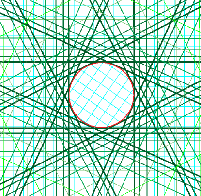
Figure 3: (Color online) A circular grain boundary can be decomposed into a series of flat walls whose density decays as $1/\Delta^{3}$ away from the center of the cylindrical cell.

A more complicated example is the case where one cuts out a cylindrical portion of radius $R$ inside a crystal with the axis of symmetry pointing along $\hat{\mathbf{z}}$, rotates it, and pastes it back (figure 3). The resulting boundary is a circular grain boundary which can be represented in Fourier space as

$$\bm{\widetilde{\rho}}^{\text{circ}}=\mathcal{J}_{1}\left[\sqrt{k_{x}^{2}+k_{y}^{2}}\,R\right]\frac{\delta(k_{z})}{\sqrt{k_{x}^{2}+k_{y}^{2}}}\bm{E}^{z},$$ (48)

where $\mathcal{J}_{1}[\cdot]$ is the Bessel function of type 1. In this case,

$$\begin{split}a^{\text{circ}}&=\frac{i\omega_{z}}{(2\pi)^{3}\pi^{\nicefrac{{3}}{{2}}}}\,\text{e}^{-|\bm{\omega}|^{2}}\\ &\qquad\quad\times\int_{-\infty}^{\infty}\!dk^{\prime}\,k^{\prime 3}\frac{\mathcal{J}_{1}\left(|k^{\prime}\sin\theta|\,R\right)}{|k^{\prime}\sin\theta|}\delta(k^{\prime}\cos\theta)\,\text{e}^{ik^{\prime}\Delta}\\ &=\frac{i\omega_{z}\text{e}^{-|\bm{\omega}|^{2}}}{(2\pi)^{3}\pi^{\nicefrac{{3}}{{2}}}}\,\delta(\cos\theta)\underbrace{\int_{-\infty}^{\infty}\!dk^{\prime}\,|k^{\prime}|\mathcal{J}_{1}(|k^{\prime}|R)\,\text{e}^{ik^{\prime}\Delta}}_{\frac{-2iR}{(\Delta^{2}-R^{2})^{\nicefrac{{3}}{{2}}}}\Theta(\Delta-R)}\\ &=\frac{2R\,\omega_{z}\text{e}^{-|\bm{\omega}|^{2}}}{(2\pi)^{3}\pi^{\nicefrac{{3}}{{2}}}(\Delta^{2}-R^{2})^{\nicefrac{{3}}{{2}}}}\,\delta(\cos\theta)\Theta(\Delta-R).\end{split}$$ (49)

This example emphasizes the important point that we mentioned earlier, that a stress-free dislocation configuration may need to be decomposed into a continuous superposition of flat cell walls. In particular, here we represent a cylindrical wall as an infinite sum of flat walls with whose amplitudes go down as $1/\Delta^{3}$ with distance $\Delta$ away from the center of the cylinder.

References

• Eshelby (1956) J. D. Eshelby (Academic Press, San Diego, 1956), pp. 79–144.
• Kröner (1958) E. Kröner, Kintinuumstheorie der Versetzungen und Eigenspannungen (Springer Verlag, Berlin, 1958).
• Kröner (1981) E. Kröner, in Physics of Defects—Les Houches Session XXXV, 1980, edited by R. Balian, M. Kléman, and J.-P. Pourier (North Holland, Amsterdam, 1981), p. 215.
• Kosevich (1962) A. M. Kosevich, Sov. Phys. JETP 15, 108 (1962).
• Mura (1963) T. Mura, Phil. Mag. 8, 843 (1963).
• Mura (1991) T. Mura, Micromechanics of Defects in Solids (Martinus Nijhoff Publishers, The Hague, The Netherlands, 1991), chap. 1.10, 2nd ed.
• Frank (1950) F. C. Frank, Carnegie Institute of Technology Symposium on the Plastic Deformation of Crystalline Solids (Pittsburgh Report) (Office of Naval Research (NAVEXOS-P-834), 1950), pp. 150–1.
• Limkumnerd and Sethna (2006a) S. Limkumnerd and J. P. Sethna, Phys. Rev. Letters 96, 095503 (2006a).
• Limkumnerd and Sethna (2006b) S. Limkumnerd and J. P. Sethna (2006b), submitted to Journal of the Mechanics and Physics of Solids.
• Groma (1997) I. Groma, Phys. Rev. B 56, 5807 (1997).
• Bakó and Groma (1999) B. Bakó and I. Groma, Phys. Rev. B 60, 122 (1999).
• Zaiser et al. (2001) M. Zaiser, M. C. Miguel, and I. Groma, Phys. Rev. B 64, 224102 (2001).
• El-Azab (2000) A. El-Azab, Phys. Rev. B 61, 11956 (2000).
• Roy and Acharya (2005) A. Roy and A. Acharya, Journal of the Mechanics and Physics of Solids 53, 143 (2005).
• Acharya and Sawant (2006) A. Acharya and A. Sawant, Journal of the Mechanics and Physics of Solids p. In press (2006).
• Acharya and Roy (2006) A. Acharya and A. Roy, Journal of the Mechanics and Physics of Solids 54, 1687 (2006).
• Roy and Acharya (2006) A. Roy and A. Acharya, Journal of the Mechanics and Physics of Solids 54, 1711 (2006).
• Miguel et al. (2001a) M. C. Miguel, A. Vespignani, S. Zapperi, J. Weiss, and J. R. Grasso, Mater. Sci. Engr. A 309–310, 324 (2001a).
• Barts and Carlsson (1997) D. B. Barts and A. E. Carlsson, Philosophical Magazine A 75, 541 (1997).
• Gullouglu and Hartly (1993) A. N. Gullouglu and C. S. Hartly, Model. Simul. Mater. Sci. Eng. 1, 383 (1993).
• Groma and Pawley (1993a) I. Groma and G. S. Pawley, Philos. Mag. A 67, 1459 (1993a).
• Groma and Pawley (1993b) I. Groma and G. S. Pawley, Mater. Sci. Eng. A 164, 306 (1993b).
• Fournet and Salazar (1996) R. Fournet and J. M. Salazar, Physical Review B 53, 6283 (1996).
• Benzerga et al. (2004) A. A. Benzerga, Y. Bréchet, A. Needleman, and E. Van der Giessen, Modeling and Simulation in Materials Science 12, 159 (2004).
• Benzerga et al. (2005) A. A. Benzerga, Y. Bréchet, A. Needleman, and E. Van der Giessen, Acta Materialia 53, 4765 (2005).
• Groma and Bakó (2000) I. Groma and B. Bakó, Phys. Rev. Lett. 84, 1487 (2000).
• Gómez-García et al. (2006) D. Gómez-García, B. Devincre, and L. Kubin, Physical Review Letters 96, 125503 (2006).
• Miguel et al. (2001b) M. C. Miguel, A. Vespignani, S. Zapperi, J. Weiss, and J.-R. Grasso, Nature 410, 667 (2001b).
• Miguel et al. (2002) M. C. Miguel, A. Vespignani, M. Zaiser, and S. Zapperi, Phys. Rev. Letters 89, 165501 (2002).
• Weiss and Marsan (2003) J. Weiss and D. Marsan, Science 299, 89 (2003).
• Richeton et al. (2005) T. Richeton, J. Weiss, and F. Louchet, Nature Materials 4, 465 (2005).
• Sammonds (2005) P. Sammonds, Nature Materials 4, 425 (2005).
• Miguel and Zapperi (2006) M. C. Miguel and S. Zapperi, Science 312, 1151 (2006).
• Zaiser (2006) M. Zaiser, Advances in Physics 55, 185 (2006).
• Dimiduk et al. (2006) D. M. Dimiduk, C. Woodward, R. LeSar, and M. D. Uchic, Science 312, 1188 (2006).
• Hughes et al. (1998) D. A. Hughes, D. C. Chrzan, Q. Liu, and N. Hansen, Phys. Rev. Lett. 81, 4664 (1998).
• Kuhlmann-Wilsdorf and Hansen (1991) D. Kuhlmann-Wilsdorf and N. Hansen, Scripta Metall. Mater. 24, 1557 (1991).
• Hughes and Hansen (1993) D. A. Hughes and N. Hansen, Metall. Trans. A 24, 2021 (1993).
• Hughes and Hansen (1995) D. A. Hughes and N. Hansen, Scripta Metall. Mater. 33, 315 (1995).
• Hughes and Hansen (2001) D. A. Hughes and N. Hansen, Phys. Rev. Lett. 87, 135503 (2001).
• Hughes (2001) D. A. Hughes, Surface and Interface Analysis 31, 560 (2001).
• Peach and Koehler (1950) M. Peach and J. S. Koehler, Phys. Rev. 80, 436 (1950).
• Arfken and Weber (1995) G. B. Arfken and H. J. Weber, Mathematical Methods for Physicists (Academic Press, New York, NY, 1995), chap. 1, p. 84, 4th ed.
• Sethna et al. (2003) J. P. Sethna, V. Coffman, and E. Demler, Phys. Rev. B 67, 184107 (2003).
• Read and Shockley (1950) W. T. Read and W. Shockley, Phys. Rev. 78, 275 (1950).
• Read (1953) W. T. Read, Dislocations in Crystals (McGraw-Hill Book Company, Inc., New York, NY, 1953), pp. 182–3.
• Sethna and Huang (1992) J. P. Sethna and M. Huang, in 1991 Lectures in Complex Systems, SFI Studies in the Sciences of Complexity, Proc. Vol. XV, edited by L. Nadel and D. Stein (Addison Wesley, New York, 1992), pp. 267–76, cond-mat/9204010.
• Nye (1953) J. F. Nye, Act. Metall. 1, 153 (1953).