A Brownian dynamics algorithm for entangled wormlike threads

Abstract

We present a hybrid Brownian dynamics / Monte Carlo algorithm for simulating solutions of highly entangled semiflexible polymers or filaments. The algorithm combines a Brownian dynamics time-stepping approach with an efficient scheme for rejecting moves that cause chains to cross or that lead to excluded volume overlaps. The algorithm allows simulation of the limit of infinitely thin but uncrossable threads, and is suitable for simulating the conditions obtained in experiments on solutions of long actin protein filaments.

I Introduction

Experimental and theoretical studies of solutions of entangled semiflexible polymers have probed concentration regimes that are difficult to simulate by standard methods. In solutions of actin protein filaments, the typical filament length $L$ and persistence length $L_{p}$ are both of order $10\mu$m, but the chain diameter $d\simeq 8$ nm is about $10^{3}$ times smaller. For such solutions at concentrations near the isotropic-nematic transition, the actin volume fraction is of order $10^{-3}$, $cL^{3}\sim 10^{3}-10^{4}$ (where $c$ is a number of chains per unit volume), and the typical distance between chains is of order $0.1\mu m$. These conditions may be fruitfully idealized in theoretical work by considering the limit $d=0$ of uncrossable but infinitely thin threads. A simulation of these conditions with a conventional molecular dynamics (MD) or Brownian dynamics (BD) model of polymers as necklaces of nearly-tangent repulsive spherical beads (Kremer and Grest, 1990) would require a large number $N\sim L/d\sim 10^{3}$ beads per chain, and an extremely small time step in order to resolve both the strong short range repulsion and the bending forces needed to maintain angular correlations over 1000 beads. Here, we present a hybrid Brownian Dynamics (BD) / Monte Carlo (MC) algorithm for simulation of such systems of very thin threads, in which chains are represented as sequences of a much smaller number of uncrossable rods. The algorithm is designed to allow efficient simulation of the idealized limit of infinitely thin but uncrossable threads, as well as of chains with a small but nonzero steric diameter.

The article is organized as follows. Sec. II is a description of our algorithm for simulating solutions of uncrossable bead-rod chains. Sec. III is a description of the geometrical algorithms used to efficiently detect chain crossings and to calculate the distance of closest approach between rods. Sec. IV presents results of tests of the validity and computational cost of the algorithm. Sec. V is a discussion of the theory underlying the algorithm. Conclusions are summarized in Sec. VI.

II Simulation Algorithm

Our simulation method combines a Brownian dynamics time-stepping algorithm with a scheme for rejecting moves that cause chains to cross or overlap. At each step, a Brownian dynamics (BD) algorithm that has been used previously to describe non-interacting wormlike chains is used to generate a trial move for a randomly chosen chain. To simulate a solution of infinitely thin but uncrossable threads, we reject all trial moves that cause one chain to cross through another, and accept all others.

II.1 Single Chain Brownian Dynamics

The simulations use a discretized model of wormlike chains in which each chain in a solution is represented as a set of $N+1$ beads, which act as point sources of friction, connected by $N$ inextensible rods, each of which is constrained to have a fixed length $a$. Let ${\bf R}_{\mu}$ be the position of bead $\mu$ of a chain, with $\mu=1,\ldots,N+1$, and ${\bf q}_{i}={\bf R}_{i+1}-{\bf R}_{i}$ be the vector associated with rod $i$, which is constrained to have a fixed length $|{\bf q}_{i}|=a$, for all $i=1,\ldots,N$. Let ${\bf u}_{i}={\bf q}_{i}/|{\bf q}_{i}|$ be a unit tangent vector for rod $i$. The bending energy, denoted by $U_{0}$, is

$$U_{0}=-\frac{\kappa}{a}\sum_{i=2}^{N}{\bf u}_{i}\cdot{\bf u}_{i-1}\quad,$$ (1)

where $\kappa$ is the bending rigidity of the chain. The persistence length is $L_{p}=\kappa/k_{B}T$. This model approximates the bending energy of a continuous wormlike chain in the limit $a\ll L_{p}$ and $N\gg 1$.

To generate trial moves for individual chains, we use a Brownian dynamics algorithm for chains with constrained rod lengths that has used previously to study dilute solutions of both semiflexible (Everaers et al., 1999; Pasquali et al., 2001; Dimitrakopoulos et al., 2001; Shankar et al., 2002; Pasquali and Morse, 2002; Montesi et al., 2005) and flexible chains Hinch (1994). In this algorithm, changes in bead positions are calculated from a bead velocity ${\bf V}_{\mu}$ of the form

$${\bf V}_{\mu}={\bf H}_{\mu}\cdot\left[-\frac{{\partial}U_{0}}{{\partial}{\bf R}_{\mu}}+\mathcal{T}_{\mu}{\bf u}_{\mu}-\mathcal{T}_{\mu-1}{\bf u}_{\mu-1}+{\bf F}_{\mu}^{met}+\mbox{\boldmath$\eta$}_{\mu}\right].$$ (2)

Here, ${\bf H}_{\mu}$ is a mobility tensor for bead $\mu$, $\mathcal{T}_{i}$ is a tension in rod $i$, and $\mbox{\boldmath$\eta$}_{\mu}$ is a random Langevin force. ${\bf F}_{\mu}^{met}$ is a metric correction force that is required in order for this algorithm to yield the correct equilibrium distribution Fixman (1978); Hinch (1994); Pasquali and Morse (2002); Morse (2004); Montesi et al. (2005).

We use an anisotropic bead mobility tensor ${\bf H}_{\mu}$ of the form Montesi et al. (2005)

$${\bf H}_{\mu}=\frac{a}{\zeta_{\parallel}}\tilde{{\bf u}}_{\mu}\tilde{{\bf u}}_{\mu}+\frac{a}{\zeta_{\perp}}({\bf I}-\tilde{{\bf u}}_{\mu}\tilde{{\bf u}}_{\mu})\quad,$$ (3)

where $\tilde{{\bf u}}_{\mu}$ is an approximation to the unit tangent vector at bead $i$, and $\zeta_{\parallel}$ and $\zeta_{\perp}$ are friction coefficients per unit length for parallel and perpendicular motion, respectively. Montesi et al. (2005). The unit tangent $\tilde{{\bf u}}_{\mu}$ is approximated by a centered difference $\tilde{{\bf u}}_{\mu}=({\bf R}_{\mu+1}-{\bf R}_{\mu-1})/|{\bf R}_{\mu+1}-{\bf R}_{\mu-1}|$ for beads $\mu=2,\ldots,N$, and by $\tilde{{\bf u}}_{1}={\bf u}_{1}$ and $\tilde{{\bf u}}_{N+1}={\bf u}_{N}$ for the end beads.

The random force $\mbox{\boldmath$\eta$}_{\mu}$ is generated by the procedure described by Morse (2004) and Montesi et al. (2005) for generating “geometrically projected” random forces. At the beginning of each time step, an unprojected random force $\mbox{\boldmath$\eta$}_{\mu}^{\prime}$ for each bead is generated from a distribution with a vanishing mean, $\langle\mbox{\boldmath$\eta$}_{\mu}^{\prime}\rangle=0$ and a variance $\langle\mbox{\boldmath$\eta$}_{\mu}^{\prime}\mbox{\boldmath$\eta$}_{\nu}^{\prime}\rangle=2k_{B}T{\bf H}^{-1}_{\mu}\delta_{\mu\nu}/\Delta t$. The force $\mbox{\boldmath$\eta$}_{\mu}$ in Eq. (2) is a projected force of the form $\mbox{\boldmath$\eta$}_{\mu}=\mbox{\boldmath$\eta$}_{\mu}^{\prime}-\hat{\eta}_{\mu}{\bf u}_{\mu}-\hat{\eta}_{\mu-1}{\bf u}_{\mu-1}$ in which the quantities $\hat{\eta}_{1},\ldots,\hat{\eta}_{N}$ are calculated by requiring that $0={\bf u}_{i}\cdot(\mbox{\boldmath$\eta$}_{i+1}-\mbox{\boldmath$\eta$}_{i})$ for all $i=1,\ldots,N$.

The tensions $\mathcal{T}_{1},\ldots,\mathcal{T}_{N}$ are calculated, after calculation of the bending, metric, and random forces, by requiring that the rod lengths all maintain constant length, or that $0={\bf u}_{i}\cdot({\bf V}_{i+1}-{\bf V}_{i})$ for all $i=1,\ldots,N$. This yields a tridiagonal set of $N$ equations, which must be solved every time step.

Each time step for a single chain is generated by a mid-step integration algorithm originally proposed by Fixman Fixman (1978); Morse (2004). At the beginning of each time step, projected random forces are generated. Predicted mid-step bead positions are then calculated as

$${\bf R}_{\mu}^{(1/2)}={\bf R}_{\mu}^{(0)}+{\bf V}_{\mu}^{(0)}\Delta t/2$$ (4)

where ${\bf R}_{\mu}^{(0)}$ represents an initial bead position and ${\bf V}_{\mu}^{(0)}$ represent a bead velocity calculated using the initial bead positions. Final bead positions are calculated as

$${\bf R}_{\mu}^{(1)}={\bf R}_{\mu}^{(0)}+{\bf V}_{\mu}^{(1/2)}\Delta t$$ (5)

where ${\bf V}_{\mu}^{(1/2)}$ is a bead velocity computed using bending and metric forces, mobilities, and tensions that are re-calculated using the mid-step bead positions, but using the same random force $\mbox{\boldmath$\eta$}_{\mu}$ as that used to calculate the mid-step positions.

II.2 Detecting chain crossing

To simulate a solution of infinitely thin but uncrossable threads, we combine this Brownian dynamics algorithm with a scheme for rejecting moves that cause chains to cross. At every timestep, a trial move is generated for a randomly chosen polymer chain using the Brownian dynamics algorithm discussed above. The trial move is rejected, and the chain position is unchanged, if the trial move would cause any of the N rods of the chosen chain to cut through any rod of any other chain. Whether or not the move is accepted, another chain is then chosen at random, and the process is repeated. To accurately simulate Brownian motion, the time step $\Delta t$ used in the Brownian dynamics algorithm must be chosen to be small enough so that almost all of the moves are accepted. In a system containing $M$ chains, a time $\Delta t$ is taken to have elapsed every $M$ attempted chain moves.

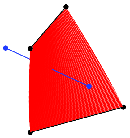
The usefulness of the algorithm relies upon the availability of an efficient method for detecting when a trial move causes one chain to cut through another. Consider an attempted move of a chain $\alpha$. To detect whether this attempted move would cause chain $\alpha$ to cut through any other chain, we consider each of the $N$ rods of chain $\alpha$ to sweep out a surface over the course of a time step. We reject the move of the chain if the surface swept out by any rod of $\alpha$ is intersected by any rod of any other polymer $\beta$, as show schematically in Figure 1.

Figure 1: Intersection of a stationary rod with the surface swept out by a moving rod

Consider the test for whether a move of rod $i$ of the moving chain $\alpha$ will cause it to cut through a rod $j$ of a stationary chain $\beta$. The line segment corresponding to the stationary rod (rod $j$ of $\beta$) may be described by a parametric equation

$${\bf r}^{\prime}(s^{\prime})={\bf c}^{\prime}+s^{\prime}{\bf q}^{\prime}.$$ (6)

where ${\bf c}^{\prime}$ is the center of the rod, ${\bf q}^{\prime}$ is the vector connecting its ends, which is of length $|{\bf q}^{\prime}|=a$, and $s^{\prime}$ is a contour length parameter with a domain $-1/2\leq s^{\prime}\leq 1/2$. The surface swept out by the moving rod (rod $i$ of $\alpha$) during a trial move can be represented by a two parameter equation,

$${\bf r}(s,t)={\bf c}(t)+s{\bf q}(t),$$ (7)

where $-1/2<s<1/2$, $t$ is a dimensionless time variable that ranges from $0$ to $1$ during the time step, and ${\bf c}(t)$ and ${\bf q}(t)$ are the center position and end-to-end vector of the rod as functions of $t$. Thus, ${\bf r}(s,0)$ and ${\bf r}(s,1)$ represent rod conformations at the beginning and end of the timestep, respectively. To define the surface swept out at intermediate times, we take ${\bf c}(t)$ and ${\bf q}(t)$ to be linear functions of $t$,

$${\bf r}(t) = {\bf c}_{0}+t\;\Delta{\bf c}$$

$${\bf q}(t) = {\bf q}_{0}+t\;\Delta{\bf q}$$ (8)

where ${\bf c}_{0}={\bf c}(0)$, ${\bf q}_{0}={\bf q}(0)$, $\Delta{\bf c}\equiv{\bf c}(1)-{\bf c}(0)$, and $\Delta{\bf q}\equiv{\bf q}(1)-{\bf q}(0)$. This is equivalent to assuming that the beads at both ends of the rod move with constant velocity from initial to final position, and that the rod is always a straight line between these two beads. The length of the rod is not exactly conserved at intermediate times, but the surfaces swept out by neighboring rods within a chain meet without gaps or overlaps along the trajectory of the shared bead.

For the surface ${\bf r}(s,t)$ swept out by the moving rod to be intersected by a stationary rod ${\bf r}^{\prime}(s^{\prime})$, the line segments ${\bf r}^{\prime}(s^{\prime})$ and ${\bf r}(s,t)$ must intersect at some time $t=t_{I}$, such that $0<t_{I}<1$, at a point of intersection for which $-1/2<s<1/2$ and $-1/2<s^{\prime}<1/2$. An efficient algorithm for determining whether such an intersection occurs for any specified pair of rods is described in Sec. III.

II.3 Rod-Rod Interactions

The algorithm for infinitely thin threads can be generalized to allow for intermolecular interactions. We consider a model in which the total potential energy is a sum of a bending energy $U_{0}$ and an interaction potential $U_{int}$. The interaction energy is taken to be a pairwise additive sum of interactions between rods,

$$U_{int}=\sum_{i>j}U(|{\bf d}_{ij}|),$$ (9)

where the sum is taken over all pairs of rods, and where the interaction energy $U(|{\bf d}_{ij}|)$ between rods $i$ and $j$ is a function of the distance of closest approach ${\bf d}_{ij}$ between those two rods. An algorithm for calculating distance of closest approach between two finite line segments, and a discussion of how this distance is defined, is given in Sec. III.

In an algorithm in which trial moves are generated using a Brownian dynamics algorithm for non-interacting chains with potential energy $U_{0}$, trial moves that do not cause chains to cross are accepted or rejected according to a Metropolis acceptance criterion that is based on the change in interaction energy: A trial move is accepted if it causes $U_{int}$ to decrease, and is accepted with a probability

$$P_{acc}=\exp[-\Delta U_{int}/(k_{B}T)]$$ (10)

if it leads to an increase $\Delta U_{int}>0$ in $U_{int}$. In the case of a hard-core interaction, a move that does not cause chain crossing is rejected if it causes the distance $|{\bf d}_{ij}|$ between any two rods to fall below a specified hard-core diameter, and accepted otherwise. Note that only the interaction energy is used in this acceptance rule, and not the change in the intramolecular bending potential, because the effect of the bending potential is already fully accounted for by the Brownian dynamics algorithm used to generate trial moves. The rationale underlying the use of such a Metropolis sampling is discussed in Sec. V.

Each step of the simulation thus involves the following sequence of operations. A trial move is generated for a randomly chosen chain. A check is performed for every rod on that chain to see if the trial move would cause intersection of that rod with any of the neighboring rods, which are identified by use of a Verlet neighbor list. The move is rejected if any intersections are found. If no intersections are found, and $U_{int}\neq 0$, the change in the interaction energy of each rod with all nearby neighbors is calculated, and the move is accepted or rejected based upon the Metropolis criterion described above.

As in simulations of systems of point particles (Allen and Tildesley, 1996), Verlet neighbor lists are used to reduce the number of rods that must be checked for intersections and for which interaction energy must be calculated. The neighbor list for each rod in the system contains all other rods for which the distance of closest approach was less than a Verlet radius $r_{l}$ when the neighbor list was constructed. The neighbor list is reconstructed whenever any bead in the simulation is found to have moved a distance greater than $r_{l}/2$ since the last update of the list. The neighbor list is constructed with the use of a linked cell list of rods, by a procedure closely analogous to that used for point particles. Optimal values of the Verlet radius for each set of parameters have been determined by extensive trial and error.

II.4 Preparation of initial states

Many of the simulations for which we have used our algorithm focus on the dynamics and stress relaxation in entangled solutions over relatively short time scales. These simulations are often run for times shorter than a reptation time due to computational limitations on our ability to simulate very crowded solutions for long times. For such short simulations to yield valid results, they must start from initial configurations that are already representative of a thermal equilibrium ensemble for the solution. Such simulations thus rely upon our ability to efficiently generate equilibrated initial states for systems that would be difficult or impossible to equilibrate by running the algorithm described above, which we use to study dynamical properties.

In the case of infinitely thin but uncrossable chains, with $U_{int}=0$, the prohibition on chain crossing has an enormous effect upon dynamics of the system, but has no effect upon the equilibrium probability distribution, since it changes neither the set of allowed microstates nor the energy of any microstate. The equilibrium distribution for a solution of such uncrossable chains is thus identical to that of a solution containing an equal number of non-interacting “phantom” chains. This distribution is characterized by random chain positions and orientations, and by a Boltzmann distribution

$$P(\cos\,\theta_{ij})=\frac{e^{(L_{p}/a)\cos\theta_{ij}}}{\int_{0}^{\pi}d\theta_{ij}\sin\theta_{ij}e^{(L_{p}/a)\cos\theta_{ij}}},$$ (11)

for the cosine $\cos\theta_{ij}={\bf u}_{i}\cdot{\bf u}_{j}$ of the angle between neighboring rods $j=i\pm 1$ within a chain. We may thus generate initial configurations for such a solution by a method used previously to generate initial configurations for dilute solutions, in which chains are grown by a process that yields an equilibrium distribution of chain conformations. The first bead of each chain is placed at random within the simulation cell, and the first rod is given a random orientation. The orientation of each subsequent rod relative to the previous one is chosen such that the cosine of the angle between these two rods is chosen from the Boltzmann distribution given in equation (11).

When $U_{int}\neq 0$, inter-molecular interactions lead to non-trivial correlations. In this case, we start with an initial configuration for a non-interacting system, generated by the method described above, and then equilibrate the system by a slithering-snake Monte-Carlo algorithm. In each attempted move of this algorithm, a rod is removed from one end (the “tail”) of a randomly chosen polymer and reattached to the other end (the “head”). The orientation of the new rod relative to that of the pre-existing end rod is chosen from the equilibrium distribution given in (11)), where $\cos\theta$ is the angle of the last joint in the chain. The resulting attempted Monte-Carlo move is accepted or rejected based on a Metropolis criterion based on the resulting change in interaction energy $U_{int}$, as given in Eq. (10) for the acceptance probability of a move that changes the interactions by an amount $U_{int}>0$. Monte Carlo equilibration is continued until every chain in the simulation box has reptated many times its own length. In the concentration range of interest, where the system is highly entangled but semi-dilute, and in which the equilibrium phase is isotropic rather than a nematic liquid crystal, almost all such Monte Carlo moves are accepted, and the system can be equilibrated quite rapidly.

III Geometrical Algorithms

III.1 Intersection

To determine whether two line segments intersect during a move, we first determine whether the two infinite lines containing these segments intersect during the time $0<t<1$ of interest. If an intersection time $0<t_{I}<1$ is found, we then calculate the contour variables $s$ and $s^{\prime}$ at the point of intersection, and determine if these lie within the two line segments that define the rod.

The efficiency of our algorithm relies upon the existence of efficient algorithms for detecting intersections between rods and calculating distances of closest approach between line segments.

An intersection between a moving line ${\bf r}(s,t)$ and a stationary non-parallel line ${\bf r}^{\prime}(s^{\prime})$ that pass through rod centers ${\bf c}(t)$ and ${\bf c}^{\prime}$, respectively, can occur at a time $t_{I}$ if the vector ${\bf c}(t_{I})-{\bf c}$ has a vanishing projection onto a vector ${\bf q}(t_{I})\times{\bf q}^{\prime}$ that is perpendicular to both lines, i.e., if

$$0=[\,{\bf c}(t_{I})-{\bf c}^{\prime}\,]\cdot[\,{\bf q}(t_{I})\times{\bf q}^{\prime}\,]$$ (12)

Substituting Eq. (II.2) for ${\bf c}(t)$ and ${\bf q}(t)$ into this condition yields a quadratic equation

$$at_{I}^{2}+bt_{I}+c=0\quad.$$ (13)

for the intersection time $t_{I}$ of the two infinite lines, in which

$$a = \Delta{\bf c}\cdot(\Delta{\bf q}\times{\bf q}^{\prime})$$

$$b = \Delta{\bf c}\cdot({\bf q}_{0}\times{\bf q}^{\prime})+[\,{\bf c}_{0}-{\bf c}^{\prime}\,]\cdot(\Delta{\bf q}\times{\bf q}^{\prime})$$

$$c = [\,{\bf c}_{0}-{\bf c}^{\prime}\,]\cdot({\bf q}_{0}\times{\bf q}^{\prime})$$ (14)

If a real solution is not found in the domain $0<t_{I}<1$, then these two lines do not intersect during the time step of interest.

If the infinite lines containing the rods do intersect at a time $0<t_{I}<1$, we must then calculate the coordinates $s$ and $s^{\prime}$ at the point of intersection, where ${\bf r}(s,t_{I})={\bf r}(s^{\prime})$. The two rods intersect only if these coordinates satisfy $-1/2<s<1/2$ and $-1/2<s^{\prime}<1/2$. We calculate the coordinates $s$ and $s^{\prime}$ as a special case of the algorithm for determining the point of closest approach of two lines, which is discussed below.

Ideally, these geometrical checks should be performed for every rod of the moving chain $\alpha$ and every other rod in the simulation box, including other rods on chain $\alpha$. The algorithm described above, however, is designed to check only for intersections of rods on a moving chain with rods on a different stationary chain. It is possible to generalize the algorithm so as to identify intersections between two moving rods. The generalization requires that the quadratic equation for $t_{I}$, equation (13), be replaced by a cubic equation. However, intersections between different parts of the same chain are expected to be rare in the systems of rodlike chains upon which we have focused and so, for simplicity, we have not implemented a check for such self-intersections.

III.2 Distance of Closest Approach

Consider two rods that correspond to line segments $-1/2\leq s\leq 1/2$ and $-1/2\leq s\leq 1/2$ of the lines

$${\bf r}(s) = {\bf c}+s{\bf q}$$

$${\bf r}^{\prime}(s^{\prime}) = {\bf c}+s^{\prime}{\bf q}^{\prime}\quad.$$ (15)

The distance of closest approach (DCA) between these two rods is the minimum magnitude $|{\bf d}(s,s^{\prime})|$ of the separation

$${\bf d}(s,s^{\prime})={\bf r}(s)-{\bf r}(s^{\prime})$$ (16)

for $-1/2\leq s\leq 1/2$ and $-1/2\leq s^{\prime}\leq 1/2$. This minimum may be obtained when $s$ and/or $s^{\prime}$ are equal to $\pm 1/2$, in which case the distance of closest approach is the distance between the end of one rod and a point along the length of the other, or the distance between two rod ends.

The first step in the calculation of this minimum distance is the identification of the coordinates $s$ and $s^{\prime}$ at the point of closest approach of the infinite lines that contain the two rods. To identify this point of closest approach, we require that

$$0 = \partial|{\bf d}|^{2}/\partial s=2{\bf q}\cdot{\bf d}(s,s^{\prime})$$

$$0 = \partial|{\bf d}|^{2}/\partial s^{\prime}=2{\bf q}^{\prime}\cdot{\bf d}(s,s^{\prime})$$ (17)

Note that this is equivalent to the geometrical requirement that the vector ${\bf d}(s,s^{\prime})$ at the point of closest approach be perpendicular to both ${\bf q}$ and ${\bf q}^{\prime}$. Substituting Eqs. (15) and (16) into these conditions yields a pair of linear equations

$$as-bs^{\prime} = d$$ (18)

$$-bs+cs^{\prime} = e$$ (19)

in which $a=|{\bf q}|^{2}$, $b={\bf q}\cdot{\bf q}^{\prime}$, $c=|{\bf q}^{\prime}|^{2}$, $d={\bf q}\cdot[{\bf c}^{\prime}-{\bf c}]$, and $e={\bf q}^{\prime}\cdot[{\bf c}-{\bf c}^{\prime}]$, which have the solution

$$s = \frac{be+cd}{ac-b^{2}}$$

$$s^{\prime} = \frac{ae+bd}{ac-b^{2}}\quad.$$ (20)

As part of the check for the intersection of two rods, we use Eq. (III.2) to calculate the coordinates $s$ and $s^{\prime}$ for pairs of lines ${\bf r}(s)={\bf r}(s,t_{I})$ and ${\bf r}^{\prime}(s^{\prime})$ that have already been shown to intersect at a time $t_{I}$, for $0<t_{I}<1$. In this case the point of closest approach is actually the point of intersection.

The distance of closest approach between the non-parallel rods is the same as that for the corresponding infinite lines if and only if the coordinates $s$ and $s^{\prime}$ at the point of closest approach of the lines satisfy the inequalities $-1/2<s,s^{\prime}<1/2$. Otherwise, the closest approach between rods may correspond to the separation between an end of one rod and a point along the length of the other (e.g., $s=1/2$ and $-1/2<s^{\prime}<1/2$), or between two rod ends (e.g., $s=1/2$ and $s^{\prime}=-1/2$). To compute the shortest distance between rods, we first use Eq. (III.2) to calculate the coordinates $s$ and $s^{\prime}$ of the point of closest approach for the infinite lines. If both $s$ and $s^{\prime}$ lie between $-1/2$ and $1/2$, we accept these values and calculate the distance $|{\bf d}(s,s^{\prime})|$. If not, we must consider one of two possible types of special cases.

The first special case occurs when one of the two coordinates $s$ and $s^{\prime}$ at the point of closest approach of two infinite lines lies within the range [-1/2,1/2], and the other does not. As an example, consider the case $s>1/2$ and $-1/2\leq s^{\prime}\leq 1/2$. In this example, the distance of closest approach will be between the rod end $s=1/2$ and some point $-1/2\leq s^{\prime}\leq 1/2$. In this example, we may identify the minimum $|{\bf d}(1/2,s^{\prime})|$ for unrestricted $s^{\prime}$ by solving linear equation (19) for $s^{\prime}$ while taking $s=1/2$. If the resulting value of $s^{\prime}$ lies outside $[-1/2,1/2]$, then the DCA between rods is obtained by setting $s^{\prime}$ to the value $s=\pm 1/2$ of the nearest end, giving a DCA equal to the distance $|{\bf d}(1/2,\pm 1/2)|$ between two rod ends.

The other type of special case occurs when neither of the coordinates at the point of closest approach of the infinite lines lies within [-1/2,1/2]. As an example, we consider $s>1/2$ and $s^{\prime}>1/2$. In this case we must locate the minima of both $|{\bf d}(1/2,s^{\prime})|^{2}$ for $-1/2\leq s\leq 1/2$ and of $|{\bf d}(s,1/2)|^{2}$ for $-1/2\leq s\leq 1/2$ by the procedure outlined above, either or both of which may yield $s=s^{\prime}=1/2$, and accept whichever yields a smaller distance.

The above reasoning applies only to non-parallel rods. Two rods are parallel if and only if the denominator in Eq. III.2 vanishes, i.e., if $ac-b^{2}=0$. For parallel rods, if $|d|\leq|a+b|/2$, then the DCA is the magnitude of the projection of ${\bf c}-{\bf c}^{\prime}$ onto the plane perpendicular to ${\bf q}$, which is given by $|{\bf c}^{\prime}-{\bf c}-{\bf q}d/a|$. If $|d|>|a+b|/2$, then the DCA is the distance between two rod ends.

IV Validation and results

IV.1 Equilibrium Properties

To show that our algorithm simulates equilibrated solutions of infinitely thin chains, we begin by analyzing results for two equilibrium properties for which analytical predictions are available.

Figure 2 shows simulation results for a histogram of the distribution of angles between neighbouring rods. The angular distributions obtained for dilute and concentrated solutions agree with each other and with equation (11) within our statistical error.

Figure 2: Probability distribution for cosine of the angle between neighboring rods of the same chain. $cL^{3}=4000$, $N=40$, $L_{p}=L$, $\zeta_{\parallel}=\zeta_{\perp}$. Legends indicate $\Delta t$ in units of $\tau_{rod}^{0}$. Values in parenthesis represent percentage of trial moves accepted.

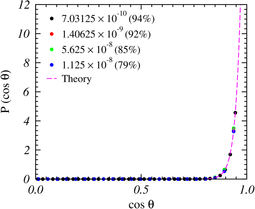
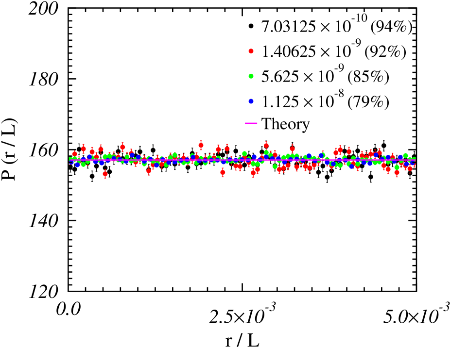
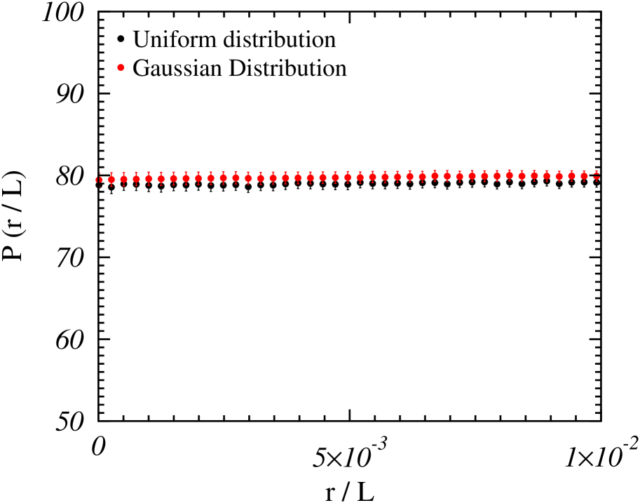
Figure 3 plots a radial distribution function obtained from simulations of entangled semiflexible polymers. The radial distribution function $P(r)$ for a test rod $i$ is defined here such that $P(r)dr$ is the probability per unit length of the test rod of finding another rod $j$ for which the points of closest approach of the lines containing the two rods lies within the line segments represented by the rods, and for which the distance of closest approach lies between $r$ and $r+dr$. We show in appendix A that $P(r)$ for a solution of infinitely thin, randomly distributed chains is given by

$$P(r)=\frac{\pi}{2}\rho$$ (21)

The radial distribution functions obtained from our simulations agree with that predicted by equation (21) to within statistical error. This agreement extends to very small values of $r$, comparable to the distance moved by the rod within a single timestep $\Delta t$, for which we might have expected our rejection scheme for preventing chain crossing to distort the equilibrium distribution.

Figure 3: Radial distribution function for rods used to discretize polymer chains. $cL^{3}=4000$, $N=40$, $L_{p}=L$, $\zeta_{\parallel}=\zeta_{\perp}$. Legends indicate $\Delta t$ in units of $\tau_{rod}^{0}$. Values in parentheses represent percentage of trial moves accepted.

IV.2 Convergence studies

Results presented in Sec. IV.1 clearly show that statistical equilibrium properties are well converged with respect to the integration timestep $\Delta t$. However, this does not necessarily imply that dynamic properties are simulated with equal accuracy.

We expect dynamical properties to be sensitive to the fraction of trial moves that are rejected, which increases with increasing time step $\Delta t$. The dependence of the fraction of moves rejected on $\Delta t$ and other parameters can be understood by the following scaling argument: The probability $P_{reject}$ that a chain of $N$ rods and length $L=Na$ will intersect another chain during a trial move is roughly $P_{reject}\sim P(r)Na\Delta r_{\perp}$, where $P(r)\sim\rho$ is the radial distribution function defined above (the number of other rods with a specified distance of closest approach per unit length of the test chain), $\Delta r_{\perp}$ is a typical magnitude for the transverse displacement of any rod of the chain, and $a\Delta r_{\perp}$ is comparable to the average area swept out by one rod. The r.m.s. transverse displacement of an individual bead or rod within a single time step of a discretized chain is of order $\Delta r_{\perp}\sim\sqrt{D_{b}\Delta t}$ of a free bead, where $D_{b}=kT/(\zeta_{\perp}a)$ is the transverse diffusivity of a single bead. By combining these expressions, we predict that the percentage of rejected moves scales as

$$P_{reject}\sim AcL^{3}\sqrt{N\Delta t/\tau_{rod}^{0}}$$ (22)

where $\tau_{rod}^{0}=\zeta_{\perp}L^{3}/(72kT)$ is the rotational diffusion time of a rigid rod of length $L$ in dilute solution, and $A$ is a universal numerical prefactor. This relation is confirmed by the data shown in Figure 4, where $P_{reject}$ is shown to be a linear function of $cL^{3}\sqrt{N\Delta t/\tau_{rod}^{0}}$ in systems with several values of $cL^{3}$ and $N$. The dotted line in this figure yields a prefactor $A\simeq 0.078$.

Figure 4: Fraction of trial moves rejected as a function of $cL^{3}\sqrt{N\Delta t/\tau_{rod}^{0}}$. Here, $\tau_{rod}^{0}=\zeta_{\perp}L^{3}/(72kT)$, $N$ is the number of rods per chain. Numbers in the legend correspond to values of $cL^{3}$ and (in parenthesis) of $N$. All simulations are for $L=L_{p}$. Dashed line represents $y=0.0775x$

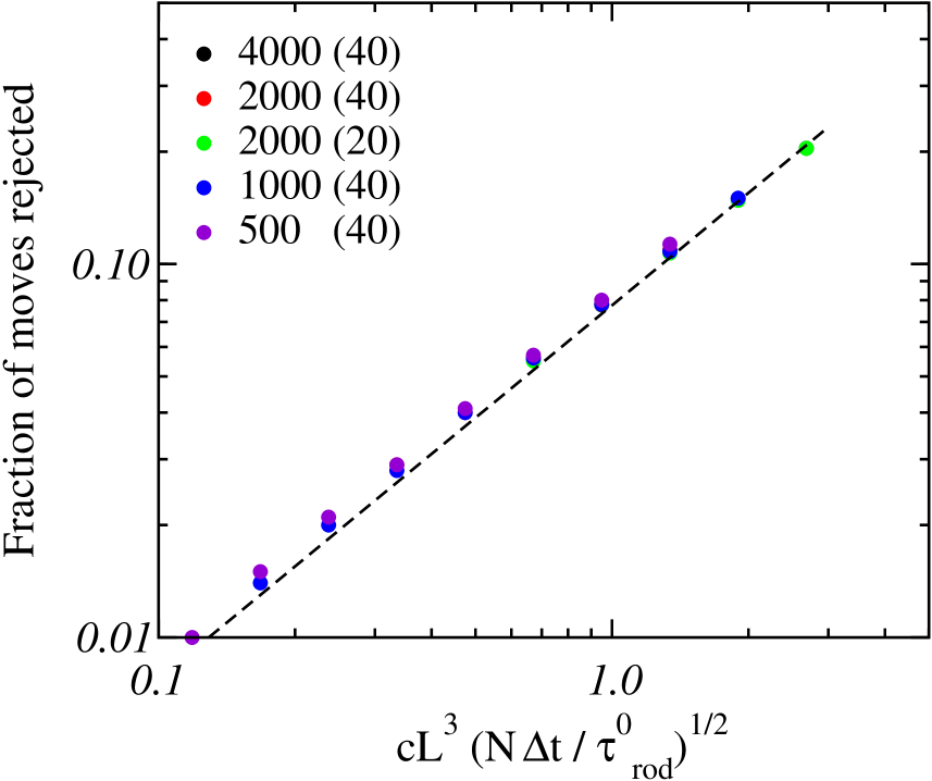
Figure 6 shows the effect of varying $\Delta t$ on a quantity $\langle\Delta d^{2}(t)\rangle$ that is approximately the mean square displacement of the middle bead of a chain along directions transverse to the tube. The quantity $\langle\Delta d^{2}(t)\rangle$ is defined to be the square of the distance of closest approach between the position of the the middle bead of a given polymer chain at a time $\tau+t$ and the contour of the same chain at an earlier time $\tau$, as shown in Figure 5. In a tightly entangled solution, the magnitude of the plateau in this quantity is a measure of the width of the tube to which the polymer is confined, and will be analyzed in detail elsewhere. Clearly, the data is well converged for all $t$ over the range of timestep values shown here, for which the rejection ratio is of order 10 %. Similar results were observed for other dynamic properties.

Figure 5: Schematic diagram defining $\langle\Delta d^{2}(t)\rangle$ for a semiflexible beadrod chain with $N=6$

Examination of this and other tests of the convergence with respect to time step led us to conclude that diffusion in tightly entangled solutions could be accurately represented, to within the statistical errors of our simulations, by choosing a time step so as to accept at least 90 % of all trial moves. In highly entangled solutions, with $cL^{3}>250$ our choice of time step is controlled by this criterion, rather than by the need to resolve the fluctuations of individual chains. Combining this criterion with Eq. (22) yields a simple prescription for calculating $\Delta t$.

Figure 6: Convergence of $\langle\Delta d^{2}(t)\rangle$ with respect to integration timestep. Legends indicate values of $\Delta t/\tau_{rod}^{0}$. Values in parenthesis represent the percentage of trial moves accepted. $L_{p}=L$, $\zeta_{\parallel}=\zeta_{\perp}$, $N=20$ for all data shown above.

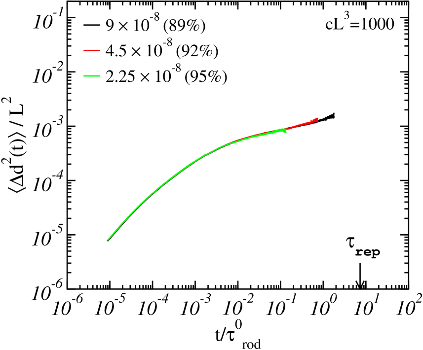
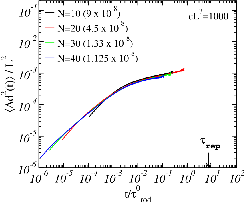
Figure 7 shows the effect of changes in the number $N$ of rods per chain on $\langle\Delta d^{2}(t)\rangle$ in solutions with $cL^{3}=1000$. The behavior of $\langle\Delta d^{2}(t)\rangle$ at very early times is, of course, very sensitive to chain discretization. At longer times, corresponding to the plateau in $\langle\Delta d^{2}(t)\rangle$, the data is less strongly affected by changes in $N$.

Figure 7: Convergence of $\langle\Delta d^{2}(t)\rangle$ with respect to chain discretization $N$. Legends indicate chain discretization $N$. Values in parenthesis represent $\Delta t/\tau_{rod}^{0}$. $\Delta t/\tau_{rod}^{0}$ has been chosen such that atleast $90\%$ of trial moves are accepted. $L_{p}=L$ and $\zeta_{\parallel}=\zeta_{\perp}$ for all data shown above.

IV.3 Computational requirements

Table I compares simulation times and memory requirements from four different simulations of solutions of semiflexible chains: (1) A simulation of isolated semiflexible chains using an algorithm developed previously for simulating dilute solutions, in which only the conformation of a single chain is stored in memory, which uses the same time stepping algorithm subroutines as those used here. (2) A simulation of 6912 phantom chains using our code for simulating entangled solutions, but without checking for intersections or interactions. The primary difference between this and simulation 1 is that it requires the positions of all of the chains to be stored simultaneously in memory. (3) A simulation of an entangled solution of 6912 uncrossable but infinitely thin semiflexible threads, in which moves that cause chains to cross are rejected. (4) A simulation of corresponding solution of uncrossable chains with repulsive excluded volume interaction, with a diameter $d/L=10^{-3}$, in which we must also calculate the change in interaction energy induced by moves that do not cause chains to cross, in order to calculate the Metropolis acceptance criterion. All simulations were performed on AMD Athlon MP processors with a CPU speed of 1.67 GHz and a cache size of 256 Kb, using a code that was implemented in Fortran 90.

From Table I, we see that the simulation of a solution of phantom chains, in which all of the chain conformations are stored but the chains do not interact, is about $8$ times slower than the equivalent simulation of individual chains. This is presumably because the entire problem no longer fits in the processors’ cache. Once the cost of this change in memory structure is paid, the addition of topological checks slows down the simulation only by a factor of about $1.5$. The addition of a small steric diameter causes an even smaller further increase. The times per rod per time step are quite comparable to the times of a few $\mu$s per particle per time step required in MD simulations of bead spring polymers with repulsive Lennard Jones interactions at liquid-like densities on the same processors.

	Verlet	Time	Memory
Simulation	$r_{l}/L$	$\mu$s /rod step	(MByte)
1) Single	$-$	$0.64$	$0.0054$
2) Phantom	$-$	$5.12$	$81.7$
3) Entangled ($d=0$)	$0.0375$	$7.61$	$96.9$
4) Entangled ($d=10^{-3}L$)	$0.0375$	$8.42$	$96.9$

Table 1: Comparison of memory and simulation times required for four different simulations of solution of chains with $L_{p}=L$ and $N=40$, with a time step $(\Delta t/\tau_{rod}^{0})=1.40625\times 10^{-9}$. Simulations (2-4) were of a system of 6912 molecules in a periodic cell of volume chosen to give $cL^{3}=4000$.

V Theoretical Background

The algorithm presented in Sec. II can be viewed either as a Brownian dynamics algorithm or as a form of Monte Carlo algorithm. The Brownian dynamics viewpoint is necessary to justify the use of the algorithm to predict dynamical properties. The Monte Carlo perspective is needed to explain the accuracy attained in results for equilibrium properties, and to justify our use of a Metropolis sampling scheme to treat the intermolecular potential.

To highlight some of the conceptual issues that arise in the discussion of our simulations, we have found it useful to also consider stochastic algorithms for a related but simpler problem of one-dimensional (1D) diffusion of a random walker with a coordinate $x(t)>0$ near a hard wall at $x=0$. The requirement that the walker cannot go through the wall is analogous to the constraint prohibiting two chains from cutting through each other. This constraint may be imposed in the 1D diffusion problem by simply rejecting moves that take the walker through the wall.

V.1 Brownian dynamics

When designing our algorithm for simulating infinitely thin uncrossable threads, we initially thought of it as a Brownian dynamics algorithm, in which the rejection of moves that lead to chain crossings was viewed as being analogous to the rejection scheme proposed above for simulating one-dimensional diffusion near a reflecting boundary.

To clarify this point of view, and its limitations, we first recall the theory underlying a conventional Brownian dynamics algorithm. In this analysis, one considers a Markov jump process for some vector of coordinates $\vec{X}=[X_{1},\ldots,X_{n}]$. in which the conditional probability distribution for any random displacement $\vec{X}\rightarrow\vec{X}+\Delta\vec{X}$ depends upon an adjustable time step $\Delta t$. The relevant set of coordinates $\vec{X}$ is the set of all bead positions in a simulation of a polymer solution or the coordinate $x$ of the random walker in the 1D diffusion problem. The probability distribution $P(\vec{X},t)$ generated by this discrete process may be shown to converge in the limit $\Delta t\rightarrow 0$ to the solution of a corresponding Fokker-Planck equation

$$\frac{\partial P}{\partial t}=-\frac{\partial(V_{i}P)}{\partial X_{i}}+\frac{\partial(D_{ij}P)}{\partial X_{i}\partial X_{j}}$$ (23)

if the first and second moments of the random displacement $\Delta X_{i}$ from a state $\vec{X}$ obey the conditions

$$V_{i}(\vec{X}) = \lim_{\Delta t\rightarrow 0}\frac{\langle\Delta X_{i}\rangle}{\Delta t}$$

$$D_{ij}(\vec{X}) = \lim_{\Delta t\rightarrow 0}\frac{\langle\Delta X_{i}\Delta X_{j}\rangle}{2\Delta t}$$ (24)

where $V_{i}(\vec{X})$ is a drift velocity vector and $D_{ij}(\vec{X})$ is a diffusivity tensor. The BD algorithm for non-interacting polymers used in our simulations was designed so as to satisfy these conditions for the drift velocity and diffusivity appropriate to a wormlike chain. Fixman (1978); Hinch (1994); Morse (2004).

In our simulations of a system of $M$ polymers, the relevant underlying Markov step is the motion of a single randomly chosen chain. The actual time elapsed during the motion of a single chain must be understood to be smaller by a factor of $M$ than the timestep of $\Delta t$ used in the underlying single-chain algorithm. This trivial rescaling of $\Delta t$ is needed to compensate for a corresponding reduction of the values of the moments $\langle\Delta X_{i}\rangle$ and $\langle\Delta X_{i}\Delta X_{j}\rangle$ in Eq. (24) for coordinates $X_{i}$ and $X_{j}$, which correspond to Cartesian components of the positions of beads on the same chain: Both of these moments are reduced by a factor of $1/M$ relative to the values obtained in a single-chain simulation because there is only a probability $1/M$ that any particular chain will move during a time step.

The derivation of the analysis outlined above relies upon the assumption that both $\vec{V_{i}}(\vec{X})$ and $D_{ij}(\vec{X})$ are smooth functions of $\vec{X}$. This condition is not satisfied by diffusion near a reflecting boundary, in which the underlying diffusion equation must either be taken to contain values of $V_{i}(\vec{X})$ and $D_{ij}(\vec{X})$ that jump discontinuously to zero at a boundary, or must be explicitly supplemented in the Fokker-Planck equation by a reflecting boundary condition. Several authors have considered how to correctly implement a reflecting boundary condition in a stochastic simulation, and proposed methods for minimizing the error arising from the presence of such a boundaryLamm and Schulten (1983); Öttinger (1989); Peters (2002). The correct probability distribution function $P(\vec{X},t)$ can actually be obtained in the limit $\Delta t\rightarrow 0$ from a variety algorithms in which the random walker is prevented from penetrating the wall. For example, for a 1D walker confined by a wall to $x>0$, the same probability distribution is obtained in the limit $\Delta t\rightarrow 0$ either by rejecting moves that yield a trial position $x<0$, or by replacing trial values of $x<0$ by $-x$. The choice of an algorithm for treating jumps near a reflecting boundary does, however, affect the magnitude of the systematic time-discretization error produced by a stochastic simulation for $\Delta t\neq 0$. In the simple 1D diffusion problem, in which each particle jumps a distance of order $\Delta x\sim\sqrt{D\Delta t}$ per time step, most “plausible” rules for treating jumps near a reflecting boundary introduce a large, ${\cal O}(1)$ error in $P(x)$ over a region of size ${\cal O}(\Delta x)$ of the boundary, and produce smaller ${\cal O}(\sqrt{\Delta t})$ errors far from the wall.

In light of this understanding, we thus initially expected our algorithm to yield a radial distribution function $P(r)$ for the distance of closest approach between pairs of uncrossable rods that deviates significantly from theoretical predictions for inter-rod distances $r$ of order the typical displacement $\Delta x$ of a single bead over one time step, which is given by $\Delta x\sim\sqrt{k_{B}T\Delta t/(a\zeta_{\perp})}$. We were surprised to find instead that there was no measurable deviation of $P(r)$ from the theoretical predictions, even at extremely small values of $r$, as shown in Figure 3. Our understanding of this result is based upon an interpretation of the algorithm as a form of Monte Carlo sampling.

V.2 Monte Carlo

Monte Carlo simulation is a method of efficiently sampling a desired equilibrium probability distribution $P_{eq}(\vec{X})$ for some set of coordinates $\vec{X}$. A Monte-Carlo simulation is based on a Markov process in which the conditional probability $T(\vec{X}_{i}\rightarrow\vec{X}_{f})$ of a transition from a state $\vec{X}_{i}$ to a state $\vec{X}_{f}$ is related to the probability of the reverse transition by a detailed balance condition (Binder, 1995)

$$P_{eq}(\vec{X}_{i})T(\vec{X}_{i}\rightarrow\vec{X}_{f})=P_{eq}(\vec{X}_{f})T(\vec{X}_{f}\rightarrow\vec{X}_{i})\quad.$$ (25)

If the Monte-Carlo jump process involves both the generation of a trial move, and a decision regarding whether to accept or reject the move, then

$$T(\vec{X}_{i}\rightarrow\vec{X}_{f})=G(\vec{X}_{i}\rightarrow\vec{X}_{f})A(\vec{X}_{i}\rightarrow\vec{X}_{f})$$ (26)

where $G(\vec{X}_{i}\rightarrow\vec{X}_{f})$ is the probability of generating a particular trial move and $A(\vec{X}_{i}\rightarrow\vec{X}_{f})$ is an acceptance probability.

V.2.1 Uncrossable Threads

We first consider the algorithm used to simulate infinitely thin uncrossable polymers. The only potential energy in the problem is the intramolecular bending energy $U_{0}$ of all of the chains. In our algorithm, trial moves are generated by a Brownian dynamics algorithm that has been designed so as to generate an equilibrium distribution for this potential. We thus consider a class of algorithms in which a BD algorithm is used to generate trial moves, and in which the BD algorithm is assumed (for the moment) to approximately satisfy detailed balance in the limit $\Delta t\rightarrow 0$. That is, we assume for the moment that

$$P_{0}(\vec{X}_{i})G(\vec{X}_{i}\rightarrow\vec{X}_{f})=P_{0}(\vec{X}_{f})G(\vec{X}_{f}\rightarrow\vec{X}_{i})$$ (27)

in the limit $\Delta t\rightarrow 0$ in which the BD algorithm is designed to yield the equilibrium distribution $P_{0}(\vec{X})$. Here, $P_{0}(\vec{X})\propto e^{-U_{0}(\vec{X})}$ is the equilibrium distribution for a solution of non-interacting wormlike chains, which is also the correct equilibrium distribution for a solution of infinitely thin but uncrossable chains with no interaction potential.

The prohibition on chain crossing is enforced by simply rejecting all moves that cause one chain to cut through another ($A=0$) and accepting all others ($A=1$). If a transition $\vec{X}_{i}\rightarrow\vec{X}_{f}$ involving the motion of the beads of one chain causes that chain to cut through another, then the hypothetical reverse move $\vec{X}_{f}\rightarrow\vec{X}_{i}$, which would involve moving the same chain from its final to initial state, would also cause a chain crossing, and so would also be rejected. If the matrix $G$ satisfies detailed balance, but certain types of moves are prohibited, then the overall transition matrix $T=GA$ will thus also satisfy detailed balance, as long as the reverse of any prohibited move is also prohibited, as is the case here. An algorithm in which a BD algorithm is supplemented by such a rejection scheme will thus satisfy detailed balance to the same extent as the underlying BD algorithm. If the BD simulation can be shown to satisfy (or nearly satisfy) detailed balance, this would explain the otherwise surprising accuracy of our results for $P(r)$.

V.2.2 Intermolecular Interactions

Our algorithm for simulating a system of chains with a short range repulsive intermolecular repulsion is an extension of the above idea. We express the total potential energy of the system as a sum

$$U=U_{0}+U_{int}$$ (28)

where $U_{0}$ is a relatively “soft” intramolecular bending energy and $U_{int}$ is a “hard” intermolecular interaction energy. The equilibrium distribution for the interacting system is of the form

$$P_{eq}(\vec{X})=P_{0}(\vec{X})e^{-U_{int}(\vec{X})/k_{B}T}$$ (29)

where $P_{0}(\vec{X})$ is the equilibrium distribution for the non-interacting gas, which is governed by the bending energy. If moves are generated with a BD algorithm that satisfies detailed balance condition (27) for non-interacting polymers, then the corresponding condition for the interacting solution can be satisfied by requiring the acceptance probability $A$ to satisfy

$$\frac{A(\vec{X}_{i}\rightarrow\vec{X}_{f})}{A(\vec{X}_{f}\rightarrow\vec{X}_{i})}=e^{-\Delta U_{int}/k_{B}T}$$ (30)

where $\Delta U_{int}\equiv U_{int}(\vec{X}_{f})-U_{int}(\vec{X}_{i})$ is the change in interaction energy. We accomplish this by supplementing our prohibition on chain crossing by the usual Metropolis scheme of taking $A(\vec{X}_{i}\rightarrow\vec{X}_{f})=1$ for $\Delta U_{int}<0$ and $A(\vec{X}_{i}\rightarrow\vec{X}_{f})=e^{-\Delta U_{int}/k_{B}T}$ for $\Delta U_{int}>0$ for moves that do not cause chains to cross. The same reasoning underlies our slithering snake algorithm for equilibrating such systems, in which the trial moves are slithering snake moves that are designed to satisfy detailed balance for non-interacting chains.

Our use of a Brownian dynamics algorithm to generate trial moves and a Metropolis acceptance scheme based on the interaction energy is useful in situations in which we wish to resolve the dynamics of chain bending, and $\Delta t$ can be made small enough to do so, but in which we do not need to resolve the dynamics of intra-chain collisions, and in which the range of repulsion between chains is so small that dynamically resolving collisions would require us to use a much smaller time step. Analogous hybrid algorithms are potentially useful in any problem in which one wishes to simulate diffusion in a comparatively soft potential in the presence of an additional steeply repulsive potential.

V.2.3 Do BD simulations satisfy detailed balance?

In appendix B, we try to answer the question of whether a valid Brownian dynamics algorithm satisfies detailed balance by considering a simplified model of one dimensional (1D) diffusion under the influence of a soft potential $U_{0}(X)$. There we consider both an algorithm in which the random force is chosen from a uniform distribution and an algorithm in which the random force is chosen from a Gaussian distribution. We find that, for this model, both algorithms satisfy detailed balance for simple diffusion in a constant potential, with no drift. In problems with nonzero deterministic drift forces, it is straightforward to show that the BD algorithm with normally distributed random forces satisfies detailed balance for any linear potential, and should thus satisfy detailed balance in the limit of $\Delta t\rightarrow 0$ for any locally linear potential. It is equally easy to show that an algorithm with a uniformly distributed random force in addition to a deterministic force does not exactly satisfy detailed balance. It is argued, however, that the small violation of detailed balance found with uniformly distributed noise should have a negligible effect when the step size is taken to be small enough to resolve variations in the soft potential. We thus conclude that, with either type of BD algorithm, the effect of any violation of detailed balance should vanish in the limit $\Delta t\rightarrow 0$ of interest.

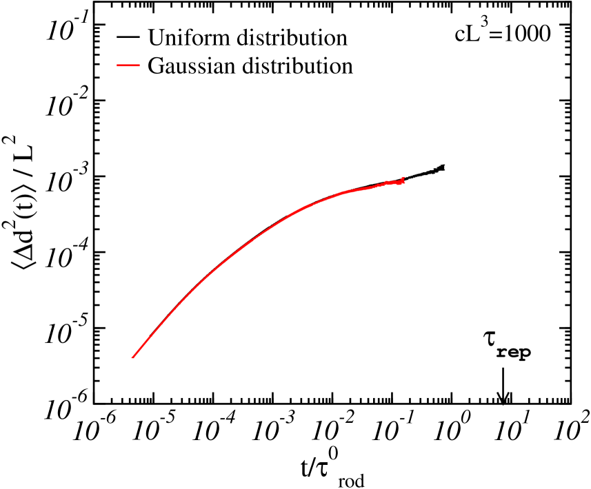
Our conclusions about the simple 1D diffusion problem are consistent with our results for simulations of entangled polymers, in which we find that the combination of single-chain BD simulation with an appropriate rejection criterion leads to results that agree to within stochastic error with theoretical predictions for the radial distribution and other equilibrium properties. In most of our simulations, we have used an unprojected random force $\mbox{\boldmath$\eta$}^{\prime}$ whose Cartesian components are chosen from a uniform distribution. An extensive series of simulations was carried out with this choice before we understood its potential theoretical significance. In order to check whether our use of uniform distribution affected our results, we also ran a smaller number of simulations with a Gaussian distribution for $\mbox{\boldmath$\eta$}^{\prime}$. Figures 8 and 9 compare results for $P(r)$ and $\langle\Delta d^{2}(t)\rangle$ obtained from simulations of infinitely thin threads using these two different noise distributions. For the value of $\Delta t$ used in our simulations, the results agree to within statistical error. Because the mathematical argument required to show that detailed balance is obtained in the limit $\Delta t\rightarrow 0$ is relatively straightforward only for BD algorithms with Gaussian-distributed random forces, however, we recommend that any future applications of a hybrid BD-MC algorithm analogous to that used here use Gaussian distributed random forces, if only to simplify any subsequent discussions of the underlying theory.

Figure 8: Effect of noise distribution on P(r). $cL^{3}=1000$, $N=20$, $L_{p}=L$, $\zeta_{\parallel}=\zeta_{\perp}$, $\Delta t/\tau_{rod}^{0}=4.5\times 10^{-8}$.

Figure 9: Effect of noise distribution on $\langle\Delta d^{2}(t)\rangle$. $cL^{3}=1000$, $N=20$, $L_{p}=L$, $\zeta_{\parallel}=\zeta_{\perp}$, $\Delta t/\tau_{rod}^{0}=4.5\times 10^{-8}$.

VI Conclusions

We have presented a hybrid algorithm for simulating highly entangled solutions of very thin uncrossable wormlike filaments. The algorithm uses a single-chain Brownian dynamics (BD) algorithm for generating trial moves. This is supplemented with a Monte Carlo-like scheme where any trial move that causes two chains to cross or that leads to excluded volume overlaps are rejected. Efficient methods were developed for checking for chain crossings and excluded volume violations. Because the algorithm is based on a Brownian dynamics time-stepping algorithm, it can be used to simulate dynamical, as well as equilibrium properties. The algorithm is expected to be much more efficient than Brownian dynamics simulation of a bead-spring model of nearly tangent beads in the limit of highly entangled solutions of extremely thin chains. Comparison with the efficiency of a molecular dynamics simulation of a bead spring model is complicated by the difference between the diffusive dynamics of our algorithm and the ballistic motion obtained in molecular dynamics of a semi-dilute solution in the absence of explicit solvent, which would lead to efficient sampling of configuration space but a loss of dynamical realism. We have used the algorithm discussed here to study dynamics and stress relaxation in highly entangled solutions Ramanathan (2006), which will be discussed elsewhere.

Appendix A Radial distribution function for rods

Consider a test rod oriented along the z-axis. Let ${\bf r}$ be the closest approach vector and ${\bf n}$ be the unit vector normal to the plane defined by the test rod and the closest approach vector. Choose an infinitesimal area on this plane, $d{\bf A}=d{\bf r}\times d{\bf z}$. Since $d{\bf r}$ is perpendicular to $d{\bf z}$ and ${\bf n}$ is perpendicular to this area unit, one can write $d{\bf A}=drdz{\bf n}$. Using geometry, one can show that the number of rods, with orientations lying between ${\bf u}$ and ${\bf u}+d{\bf u}$, that pierce this infinitesimal area is given by

$$dN_{{\bf u}}=\rho\;d{\bf A}\cdot{\bf u}\;(2)\;\frac{d^{2}{\bf u}}{4\pi}.$$ (1)

where $\rho$, as defined earlier, represents the contour length density. $d^{2}{\bf u}$ represents the solid angle subtended by ${\bf u}$ and ${\bf u}+d{\bf u}$ and is given by $d^{2}{\bf u}=\sin\theta d\theta d\phi$, where $\theta$ represents the angle between ${\bf u}$ and the z-axis and $\phi$ represents the azimuthal angle. The factor $4\pi$ in the denominator is obtained by integrating with respect to $d^{2}{\bf u}$ over the surface of a sphere. The factor of $2$ in the numerator arises because of the need to count for rods with both orientations, ${\bf u}$ and $-{\bf u}$. Substituting for $d^{2}{\bf u}$ and $d{\bf A}$ from above while noting that ${\bf n}\cdot{\bf u}=\cos(90^{o}-\theta)=\sin\theta$ and integrating equation (1) over $d\theta$, $d\phi$, we obtain the radial distribution function given in Eq. (21).

Appendix B Simulation of one-dimensional diffusion

In this appendix, we consider whether a very simple Brownian dynamics algorithm satisfies detailed balance when applied to one dimensional (1D) diffusion. We consider the use of a hybrid BD-MC algorithm analogous to that discussed in the body of the paper to describe the diffusion of a particle with a position $X(t)$ which is subjected to both a slowly-varying (or “soft”) potential $U_{0}(X)$ and an arbitrary steep repulsive (or “hard”) potential $U_{1}(X)$ that represents the walls of a confining 1D box. To represent a box of length $L$ with hard walls, we might take $U_{1}(X)$ to vanish for $-L/2<X<L/2$, and to diverge outside this domain. We consider an algorithm in which trial moves are generated by a Brownian dynamics algorithm that is obtained by discretizing the Langevin equation

$$\zeta dX=\left[F_{0}(X)+\eta(t)\right]dt$$ (1)

where $\zeta$ is a friction coefficient, $X$ is the particle position, $\eta(t)$ is a random force, and $F_{0}(X)=-dU(X)/dX$ is a force arising from the soft potential. Each time step, we generate a trial step $X_{i}\rightarrow X_{f}$ of magnitude

$$\zeta\Delta X=\left[F_{0}(X_{i})+\eta\right]\Delta t$$ (2)

where $\Delta X=X_{f}-X_{i}$, and where $\eta$ is chosen from a distribution $P(\eta)$ with moments $\langle\eta\rangle=0$ and $\langle\eta^{2}\rangle=2k_{B}T\zeta/\Delta t$. Here, we consider whether the resulting jump probability satisfies the detailed balance condition $P_{0}(X_{i})G(X_{i}\rightarrow X_{f})=P_{0}(X_{f})G(X_{f}\rightarrow X_{i})$, where $P_{0}(X)\propto e^{-U_{0}(X)/k_{B}T}$. If, in a given step, we generate a trial move $X_{i}\rightarrow X_{f}$ using a force $\eta^{+}$, we must consider a hypothetical reverse move in which the random force $\eta^{-}$ must satisfy

$$\eta^{+}+F_{0}(X_{i})=-[\eta^{-}+F_{0}(X_{f})]$$ (3)

in order to generate a displacement $-\Delta X$.

If the probability distribution $P(\eta)$ for the random force $\eta$ is a Gaussian,

$$P(\eta)\propto\exp\left(-\eta^{2}/(4k_{B}T\zeta)\right)\;,$$ (4)

it is straightforward to show that

$$\frac{G(X_{i}\rightarrow X_{f})}{G(X_{f}\rightarrow X_{i})}=e^{-\bar{F}[\eta+\bar{F}]\Delta t/(\zeta k_{B}T)}\;$$ (5)

where $\bar{F}\equiv[F_{0}(X_{i})+F_{0}(X_{f})]/2$. To lowest order in $\Delta X$, we may approximate the change in energy $\Delta U\equiv U(X_{F})-U(X_{i})$ by $\Delta U\simeq\bar{F}\delta X$ and approximate $\Delta X\simeq[\eta+\bar{F}]\Delta t$ to show that

$$\frac{G(X_{i}\rightarrow X_{f})}{G(X_{f}\rightarrow X_{i})}\simeq e^{-\Delta U_{0}/k_{B}T}\quad.$$ (6)

The algorithm thus approximately satisfies the detailed balance condition in the limit $\Delta t\rightarrow 0$ of interest, and can be shown to exactly satisfy detailed balance in the special case of a constant force $F_{0}(X)$.

We next consider a uniformly distributed random force, for which $P(\eta)=1/(2E)$ over a range $-E<\eta<E$, where $E=\sqrt{6\zeta k_{B}T/\Delta t}$. This algorithm clearly does not exactly satisfy detailed balance, since a step for which the random force $\eta^{+}$ that generates the forward trial move is near one of the boundaries $\pm E$ can sometimes be reversed only by a random force $\eta^{-}$ that lies outside the allowed range $[-E,E]$. An algorithm in which the reverse of an allowed step is sometimes not allowed clearly cannot exactly satisfy detailed balance. In the limit of small force $F_{0}$, however, this violation becomes small, insofar as it only affects a small fraction of all jumps for which $\eta$ falls within a narrow range of values near its maximum or minimum allowed value of $\pm E$. In the special case of a vanishing force, or constant potential $U_{0}(X)$, detailed balance is recovered, for any distribution with the symmetry $P(\eta)=P(-\eta)$, including a uniform distribution.

In order to assess the importance of this violation of detailed balance for an algorithm with uniformly distributed noise and a spatially varying potential $U_{0}$, we must consider the implications of our original assumption that $U_{0}(X)$ is a “soft” potential and $U_{1}(x)$ is “hard”. The effect of a deterministic force $F$ becomes comparable to or greater than that of diffusion only when applied over a characteristic distance of order $k_{B}T/F$ or greater, for which the corresponding potential energy exceeds $k_{B}T$, or over a corresponding time scale of order $k_{B}T\zeta/F^{2}$, for which the displacement $Ft/\zeta$ caused by drift exceeds the root-mean-squared displacement $\sqrt{Dt}$ caused by diffusion. If the range of the hard potential $U_{1}$ is much less than the characteristic length scale $k_{B}T/F$, then we expect the existence of a nonzero force $F$ to have negligible effect upon the structure of the probability distribution within the narrow boundary layer in which the hard repulsive potential is important, other than to change an overall prefactor that is sensitive to the nature of the far field. Within this boundary layer, the form of the probability distribution is instead determined by a balance between the repulsive potential $U_{1}$ and diffusion. Since the form of the equilibrium distribution produced by this balance can be correctly simulated by an algorithm with no drift, which does satisfy detailed balance, we expect the addition of a small drift term (and a correspondingly small violation of detailed balance) to have little effect upon the form of the probability distribution near the boundary, as long as the range of the “hard” potential $U_{1}$ is much less than the characteristic length scale $k_{B}T/F$ of the “soft” potential.

For completeness we may also consider the case in which the range of the repulsive potential $U_{1}$ is actually comparable to that the characteristic length scale of the soft potential $U_{0}$. Since we rely on a BD algorithm to resolve the effect of potential $U_{0}$, we assume that we will choose a step size $\Delta t$ such that the corresponding spatial step $\Delta X\simeq\sqrt{D\Delta t}$ is much less than any length characteristic of potential $U_{0}$. If the characteristic length scales of $U_{0}$ and $U_{1}$ are comparable, however, then we will automatically have chosen the step size small enough so that potential $U_{1}$ changes by much less than $k_{B}T$ per step. It can be shown in this case, by considering the effect of the acceptance criterion in the limit of a soft potential $U_{1}$, that the overall transition matrix $T=GA$ for the resulting algorithm satisfies the conditions on the first and second moments necessary to obtain a valid Brownian dynamics algorithm for the total potential $U_{0}+U_{1}$. In this case, the hybrid algorithm can thus be justified as a valid form of Brownian dynamics simulation, and the violation of detailed balance becomes irrelevant.

References

- Kremer and Grest (1990) K. Kremer and G. Grest, J. Chem. Phys. 92, 5057 (1990).
- Everaers et al. (1999) R. Everaers, F. Julicher, A. Ajdari, and A. C. Maggs, Phys. Rev. Lett. 82, 3717 (1999).
- Pasquali et al. (2001) M. Pasquali, V. Shankar, and D. C. Morse, Phys. Rev. E 64, 020802 (2001).
- Dimitrakopoulos et al. (2001) P. Dimitrakopoulos, J. F. Brady, and Z. G. Wang, Phys. Rev. E. 64, 050803(R) (2001).
- Shankar et al. (2002) V. Shankar, M. Pasquali, and D. C. Morse, J. Rheol. 46, 1111 (2002).
- Pasquali and Morse (2002) M. Pasquali and D. C. Morse, J. Chem. Phys. 116, 1834 (2002).
- Montesi et al. (2005) A. Montesi, M. Pasquali, and D. C. Morse, J. Chem. Phys. 122, 084903 (2005).
- Hinch (1994) E. J. Hinch, J. Fluid. Mech. 271, 219 (1994).
- Fixman (1978) M. Fixman, J. Chem. Phys. 69, 1527 (1978).
- Morse (2004) D. C. Morse, Advances in Chemical Physics 128, 65 (2004).
- Allen and Tildesley (1996) M. P. Allen and D. J. Tildesley, Computer Simulation of Liquids (Clarendon Press, 1996).
- Lamm and Schulten (1983) G. Lamm and K. Schulten, J. Chem. Phys. 78, 2713 (1983).
- Öttinger (1989) H.-C. Öttinger, J. Chem. Phys. 91, 6455 (1989).
- Peters (2002) E. Peters, Phys. Rev. E 66, 056701 (2002).
- Binder (1995) K. Binder, Monte Carlo and Molecular Dynamics Simulations in Polymer Science (Oxford University Press Inc., 1995).
- Ramanathan (2006) S. Ramanathan, Ph.D. thesis, University of Minnesota (2006).