Magneto-quantum oscillations of the conductance of a tunnel point-contact in the presence of a single defect.

Abstract

The influence of a strong magnetic field $H$ to the conductance of a tunnel point contact in the presence of a single defect has been considered. We demonstrate that the conductance exhibits specific magneto-quantum oscillations, the amplitude and period of which depend on the distance between the contact and the defect. We show that a non-monotonic dependence of the point-contact conductance results from a superposition of two types of oscillations: A short period oscillation arising from the electrons being focused by the field $H$ and a long period oscillation originated from the magnetic flux passing through the closed trajectories of electrons moving from the contact to the defect and returning back to the contact.

I Introduction

The presence of a single defect in the vicinity of a point contact manifests itself in an oscillatory dependence of the conductance $G$ on the applied voltage $V$ and the distance between the contact and the defect. Conductance oscillations originate from quantum interference between electrons that pass directly through the contact and electrons that are backscattered by the defect and again forward scattered by the contact. The reason of the oscillations of $G(V)$ is a dependence of the phase shift between two waves on the electron energy, which depends on the bias $eV$. This effect has been observed experimentally Ludoph1 ; Untiedt ; Ludoph ; Kempen and investigated theoretically Avotina1 ; Namir ; Avotina2 ; Avotina3 ; Avotina4 . In an earlier paper Avotina1 we demonstrated that this $G(V)$ dependence can actually be used to determine the exact location of a defect underneath a metal surface by means of scanning tunnelling microscopy (STM). A more elaborate version of this method Avotina4 that takes the Fermi surface anisotropy into account corresponds quite well with experimental observations Wend . Here we consider another way to change the phase shift between the interfering waves: By applying an external magnetic field $\mathbf{H}$ we expect to observe oscillations of the conductance as a function of the field $\mathbf{H.}$

It is well known that a high magnetic field $\mathbf{H}$ fundamentally changes the kinetic and thermodynamic characteristics of a metal LAK ; Abrikosov . When speaking of a high magnetic field one usually assumes two conditions to be fulfilled. The first one is that the radius of the electron trajectory, $r_{H},$ is much smaller than the mean free path of electrons, $l$. This condition implies that electrons move along spiral trajectories between two scattering events, such as by defects or phonons. This change in character of the electron motion results, for example, in the phenomenon of magnetoresistance LAK ; Abrikosov . The second condition requires that the distance between the magnetic quantum levels, the Landau levels, $\hbar\Omega$ ($\Omega$ is the frequency of the electron motion in the magnetic field $H$) is larger than the temperature $k_{\mathrm{B}}T.$ Under this condition oscillatory quantum effects, such as the de Haas-van Alphen and Shubnikov-de Haas oscillations, can be observed LAK ; Abrikosov . At which actual value the field $H$ can be identified as a high depends on the purity of the metal, its electron characteristics and the temperature of the experiment. Typically, the high field condition requires fields values above 10T for metals at low temperatures, $T\simeq 1$K, while for a pure bismuth monocrystal (a semimetal) a field of $H\simeq 0.1$T is sufficient to satisfy the two conditions mentioned.

A high magnetic field $\mathbf{H}$ influences the current spreading of the electrons passing through the contact. If the vector $\mathbf{H}$ is parallel to the contact axis, the electron motion becomes quasi-one-dimensional. Electrons then move inside a ‘tube’ with a diameter defined by the contact radius, $a$, and the radius $r_{H}$. The three-dimensional spreading of the current is restored by elastic and inelastic scattering processes. As shown in Bogachek , for $r_{H}\ll a$ and $r_{H}\ll l$, the contact resistance increases linearly with the magnetic field, in contrast to bulk samples for which the resistance increases as $H^{2}$. The Shubnikov-de Haas oscillations in the resistance of ‘large’ contacts (defined by $a\gg\lambda_{\mathrm{F}}$, with $\lambda_{\mathrm{F}}$ the electron Fermi wave length) were considered theoretically in Refs. Bogachek1 ; Bogachek2 . Experimentally, a point-contact magnetoresistance linear in $H$ as well as Shubnikov-de Haas oscillations were observed for bismuth Andr .

In this paper we consider the influence of a high magnetic field on the linear conductance (Ohm’s law approximation, $V\rightarrow 0$) of a tunnel point contact in the presence of a single defect, with the magnetic field directed along the contact axis. We demonstrate that the conductance exhibits magneto-quantum oscillations, the amplitude and period of which depend on the distance between the contact and the defect. We show that the non-monotonic dependence of the conductance $G(H)$ results from the superposition of two types of oscillations: (a) A short period oscillation arising from electrons being focused by the field $H$ and (b) a long period oscillation of Aharonov-Bohm-type originating from the magnetic flux passing through the area enclosed by the electron trajectories from contact to defect and vice versa.

In Sec. II we will discuss the model of a tunnel point-contact and find the electron wave function in the limit of a high potential barrier at the contact. The interaction of the electrons with a single impurity placed nearby the contact is taken into account by perturbation theory, with the electron-impurity interaction as the small parameter. A general analytical expression for the dependence of conductance, $G(H)$, on the magnetic field $H$ is obtained in Sec. III. It describes $G(H)$ in terms of the distance between contact and defect and the value of the magnetic field. The physical interpretation of of the general expression for the conductance can be obtained from the semiclassical asymptotics given in this Section. In Sec. IV we conclude by discussing our results and the feasibility of finding the predicted effects experimentally.

II Model and electron wave function

Let us consider a point-contact centered at the point $\mathbf{r}=0$, as illustrated in Fig. 1.

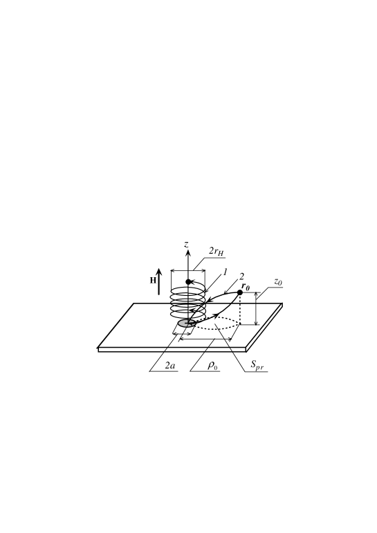
Figure 1: Model of a tunnel point-contact. The upper and lower metal half-spaces are separated by an inhomogeneous barrier (Eq. (1)) that allows electron tunneling mainly in a small region with a characteristic radius $a$, which defines the tunneling point contact. A single defect is placed inside the upper metal at the position $\mathbf{r}_{0}$. Electron trajectories in the magnetic field are shown schematically.

We use cylindrical coordinates $\mathbf{r}=\left(\rho,\varphi,z\right)$ with the $z$-axis directed along the axis of the contact. The potential barrier in the plane $z=0$ is taken to be defined by a $\delta$-function of the form,

$$U(\rho,\varphi,z)=Uf(\rho)\delta(z).$$ (1)

In order to allow for the current to flow only through a small region near the point $\mathbf{r}=0$ we choose the model function

$$f(\rho)=e^{\rho^{2}/a^{2}},$$ (2)

where the small $a$ specifies the characteristic radius of the contact. A point-like defect is placed at the point $\mathbf{r}=\mathbf{r}_{0}$ in vicinity of the interface in the half-space $z>0$, see Fig. 1. The scattering of electrons with the defect is described by a potential $D(\left|\mathbf{r}-\mathbf{r}_{0}\right|)$, which is localized near the point $\mathbf{r}=\mathbf{r}_{0}$ in a small region with a characteristic radius, which is of the order of the Fermi wave length $\lambda_{\mathrm{F}}.$ The screened Coulomb potential is an example of such kind of dependence of $D(r)$ Kittel . It is widely used to describe charge point defects (impurities) in metals.

We assume that the transmission probability of electrons through the barrier, Eq. (1), is small such that the applied voltage drops entirely over the barrier. We can then take the electric potential as a step function $V(z)=V\,\Theta(-z)$. The magnetic field is directed along the contact axis, $\mathbf{H}=(0,0,H)$. In cylindrical coordinates the vector-potential $\mathbf{A}$ has components $A_{\varphi}=H\rho/2,$ $A_{z}=A_{\rho}=0.$

The Schrödinger equation for the wave function $\psi(\rho\mathbf{,}\varphi,z)$ is given by

$$-\frac{\hbar^{2}}{2m^{\ast}}\left[\frac{1}{\rho}\frac{\partial}{\partial\rho}\left(\rho\frac{\partial\psi}{\partial\rho}\right)+\frac{\partial^{2}\psi}{\partial z^{2}}+\frac{1}{\rho^{2}}\frac{\partial^{2}\psi}{\partial\varphi^{2}}\right]-\frac{i\hbar\Omega}{2}\frac{\partial\psi}{\partial\varphi}+$$ (3)

$$+\left(\frac{m^{\ast}\Omega^{2}}{8}\rho^{2}+U(\rho\mathbf{,}z)+D(\rho\mathbf{,}\varphi,z)\right)\psi=\left(\varepsilon+\sigma\mu_{\mathrm{B}}H\right)\psi,$$

where $\Omega=eH/m^{\ast}c$; $\varepsilon$ and $m^{\ast}$ are the electron energy and effective mass, respectively, and $e$ is the absolute value of the electron charge, $\sigma=\pm 1$ corresponds to different spin directions, $\mu_{\mathrm{B}}=e\hbar/2m_{0}c$ is the Bohr magneton, where $m_{0}$ is the free electron mass. Hereinafter assuming that $\mu_{\mathrm{B}}H/\varepsilon_{\mathrm{F}}\simeq\lambdabar_{\mathrm{F}}/r_{H}\ll 1$ we will neglect by the term $\sigma\mu_{\mathrm{B}}H$ in Eq.(3).

In order to solve Eq. (3) in the limit of a high potential barrier we use the method that was developed in Refs. KMO ; Avotina1 . To first order approximation in the small parameter $\hbar p_{z}/m^{\ast}U\ll 1$, which leads to a small electron tunnelling probability $T\approx\left(\hbar p_{z}/m^{\ast}U\right)^{2}\ll 1$, the wave function $\psi$ can be written in the form,

$$\psi(\rho,\varphi,z) = \psi_{0}(\rho,\varphi,z)+\varphi^{(-)}(\rho,\varphi,z)\qquad\,\,(z<0),$$ (4)

$$\psi(\rho,\varphi,z) = \varphi^{(+)}(\rho,\varphi,z)\qquad\qquad\qquad\qquad(z>0),$$ (5)

where $\psi_{0}$ does not depend on $U$, but $\varphi^{(\pm)}\sim 1/U.$ In Eq. (4) $\psi_{0}$ is the wave function in the absence of tunnelling, for $U\rightarrow\infty$. It satisfies the boundary condition $\psi_{0}(\rho,\varphi,0)=0$ at the interface. Using the well known solution of the Schrödinger equation for an electron in a magnetic field LandauQM the energy spectrum and wave function $\psi_{0}$ are given by,

$$\varepsilon=\varepsilon_{mn}+\frac{p_{z}^{2}}{2m^{\ast}},\qquad\varepsilon_{mn}=\hbar\Omega\left(n+\frac{m+\left|m\right|+1}{2}\right),$$ (6)

$$\psi_{0}(\rho,\varphi,z)=e^{im\varphi}\left(e^{\frac{i}{\hbar}p_{z}z}-e^{-\frac{i}{\hbar}p_{z}z}\right)R_{nm}(\rho),$$ (7)

where

$$R_{nm}(\rho)=\left[\frac{\left(n\right)!}{\left(\left|m\right|+n\right)!}\right]^{1/2}\exp\left(-\frac{\xi}{2}\right)\xi^{\left|m\right|/2}L_{n}^{\left|m\right|}(\xi).$$ (8)

Here, $\xi=\rho^{2}/2a_{H}^{2}$, and $L_{n}^{\left|m\right|}(\xi)$ are the generalized Laguerre polynomials, $a_{H}=\sqrt{\hbar/m^{\ast}\Omega}$ is the quantum magnetic length, $n=0,1,2...,$ $m=0,\pm 1,\pm 2...$, and $p_{z}$ is the electron momentum along the vector $\mathbf{H}$. The functions (8) are orthogonal. We use a normalization of the wave function (8) such that $R_{n0}(0)=1.$

The function $\varphi^{(-)}(\rho,\varphi,z)$ in Eq. (4) describes the correction to the reflected wave as a result of a finite tunnelling probability and $\varphi^{(+)}(\rho,\varphi,z)$, Eq. (5), is the wave function for the electrons that are transmitted through the contact. The wave functions (4) and (5) should be matched at the interface $z=0.$ For large $U$ the resulting boundary conditions for the functions $\varphi^{(-)}$ and $\varphi^{(+)}$ become KMO ,

$$\varphi^{(-)}(\rho,\varphi,0)=\varphi^{(+)}(\rho,\varphi,0);$$ (9)

$$ip_{z}=\frac{m^{\ast}U}{\hbar}f(\rho)\varphi^{(+)}(\rho,\varphi,0).$$ (10)

In order to proceed with further calculations we assume that the electron-impurity interaction is small and use perturbation theory Avotina1 . In the zeroth approximation in the defect scattering potential the function $\varphi_{0}^{(+)}$ can be found by means of the expansion of the function $\varphi_{0}^{(+)}(\rho,\varphi,0)$ over the full set of orthogonal functions $R_{nm}(\rho)$, Eq. (8), and $\varphi_{0}^{(+)}(\rho,\varphi,z)$ is given by

$$\varphi_{0}^{(+)}(\rho,\varphi,z)=-\frac{i\hbar p_{z}}{m^{\ast}U}\frac{1}{2\pi a_{H}^{2}}\sum\limits_{n^{\prime}=0}^{\infty}F_{nn^{\prime},m}e^{im\varphi}R_{n^{\prime}m}(\rho)\exp\left(\frac{i}{\hbar}p_{z,n^{\prime}m}z\right),\text{ \ }$$ (11)

for $z\neq 0$. Here,

$$p_{z,nm}=\sqrt{2m^{\ast}\left(\varepsilon-\varepsilon_{nm}\right)},$$ (12)

and

$$F_{nn^{\prime},m}=\int\limits_{0}^{a}d\rho\;\rho f(\rho)R_{nm}(\rho)R_{n^{\prime}m}^{\ast}(\rho).$$ (13)

For the model function $f(\rho)$ of Eq. (2) the integral (13) can be evaluated and the function $F_{nn^{\prime},m}$ takes the form

$$F_{nn^{\prime},m} = \left[\frac{\left(\left|m\right|+n\right)!\left(\left|m\right|+n^{\prime}\right)!}{\left(n\right)!\left(n^{\prime}\right)!}\right]^{1/2}\frac{\pi a^{2}}{\left(\left|m\right|\right)!}\left(\frac{a^{2}}{2a_{H}^{2}}\right)^{\left|m\right|}\left(1-\frac{a^{2}}{2a_{H}^{2}}\right)^{\left|m\right|+1+n+n^{\prime}}\times$$

$${}_{2}F_{1}\left(\left|m\right|+1+n^{\prime},\left|m\right|+1+n,\left|m\right|+1,\frac{a^{4}}{4a_{H}^{4}}\right),$$

where ${}_{2}F_{1}(a,b,c,\xi)$ is a hypergeometric function. By using the procedure developed in the Ref. Avotina1 we find the wave function $\varphi^{(+)}(\rho,\varphi,z)$ at $z>z_{0}$ accurate to $g$

$$\varphi^{(+)}(\rho,\varphi,z) = \varphi_{0}^{(+)}(\rho,\varphi,z)+\frac{im^{\ast}g}{2\pi\hbar}\frac{1}{2\pi a_{H}^{2}}\varphi_{0}^{(+)}(\rho_{0},\varphi_{0},z_{0})\times$$

$$\sum\limits_{n^{\prime}=0}^{\infty}\sum\limits_{m^{\prime}=-\infty}^{\infty}\frac{e^{im^{\prime}\left(\varphi-\varphi_{0}\right)}}{p_{z}^{\prime}}R_{n^{\prime}m^{\prime}}(\rho)R_{n^{\prime}m^{\prime}}^{\ast}(\rho_{0})\left(e^{\frac{i}{\hbar}p_{z}^{\prime}\left(z-z_{0}\right)}-e^{\frac{i}{\hbar}p_{z}^{\prime}\left(z+z_{0}\right)}\right),$$

where

$$g=\int d\mathbf{r}^{\prime}D(\left|\mathbf{r}^{\prime}-\mathbf{r}_{0}\right|)$$ (16)

is the interaction constant for the scattering of the electron with the impurity. We proceed in Sec. III to calculate the total current through the contact and the point-contact conductance, using the wave function (II).

III Total current and point-contact conductance

The electrical current $I(H)$ can be evaluated from the electron wave functions of the system, $\psi$ ISh . We shall also assume that the applied bias $eV$ is much smaller than the Fermi energy, $\varepsilon_{\mathrm{F}}$, and calculate the conductance in linear approximation in $V$. In this approximation we find

$$I(H)=-\frac{2\left|e\right|^{3}HV}{\left(2\pi\hbar\right)^{2}c}\sum\limits_{n=0}^{\infty}\sum\limits_{m=-\infty}^{\infty}\int dp_{z}I_{nm,p_{z}}\Theta(p_{z})\frac{\partial n_{\mathrm{F}}(\varepsilon)}{\partial\varepsilon}.$$ (17)

Here

$$I_{nm,p_{z}}=\frac{\hbar}{m^{\ast}}\int\limits_{0}^{2\pi}d\varphi\int\limits_{0}^{\infty}\rho\,d\rho\ \mathrm{\mathop{\mathrm{R}e}}\left(\left(\varphi^{(+)}\right)^{\ast}\frac{\partial\varphi^{(+)}}{\partial z}\right)$$ (18)

is the probability current density in the $z$ direction, integrated over plane $z=$ constant; $n_{\mathrm{F}}(\varepsilon)$ is the Fermi distribution function. For a small contact, $a\ll a_{H}$, Eq. (17) can be simplified. The largest term in the parameter $a^{2}/2a_{H}^{2}\ll 1$ in Eq. (17) corresponds to $m=0$, for which the Eq. (II) takes the form $F_{nn^{\prime},0}\thickapprox\pi a^{2}$.

After space integration over a plane at $z>z_{0},$ where the wave function (II) can be used, we obtain the current density (18). At low temperatures, $T\rightarrow 0$, the integral over $p_{z}$ in Eq. (17) can be easily calculated. The point-contact conductance, $G$, is the first derivative of the total current $I$ over the voltage $V:$

$$G(H) = G_{c}\left(1+\frac{gm^{\ast}}{4\pi^{3}N(\varepsilon_{\mathrm{F}})\hbar^{2}a_{H}^{4}}\mathop{\mathrm{I}m}\left(\sum\limits_{n^{\prime}=0}^{n_{\max}(\varepsilon_{\mathrm{F}})}\chi(\varepsilon_{\mathrm{F}},n^{\prime},\mathbf{r}_{0})\right)\right.\times$$

$$\left.\mathop{\mathrm{R}e}\sum\limits_{n^{\prime\prime}=0}^{\infty}\chi(\varepsilon_{\mathrm{F}},n^{\prime\prime},\mathbf{r}_{0})\right).$$

Here

$$\chi(\varepsilon,n,\mathbf{r}_{0})=R_{n0}(\rho_{0})\exp\left(\frac{i}{\hbar}p_{z,n0}z_{0}\right),$$ (20)

$N(\varepsilon)$ is the number of electron states per unit volume,

$$N(\varepsilon,H)=\frac{4\left|e\right|H}{\left(2\pi\hbar\right)^{2}c}\sum\limits_{n=0}^{n_{\max}(\varepsilon)}\sqrt{2m\left(\varepsilon-\varepsilon_{n0}\right)},$$ (21)

and $n_{\max}(\varepsilon)=\left[\frac{\varepsilon}{\hbar\Omega}\right]$ is the maximum value of the quantum number $n$ for which $\varepsilon_{n0}<\varepsilon,$ and $\left[x\right]$ is the integer part of the number $x.$ The constant $G_{c}$ is the conductance in absence of a defect,

$$G_{c}(H)=\pi^{3}e^{2}\hbar^{3}\left(\frac{a^{2}N(\varepsilon_{\mathrm{F}})}{2m^{\ast}U}\right)^{2}.$$ (22)

The second term in brackets in Eq. (III) describes the oscillatory part of the conductance, $\Delta G(H)=G(H)-G_{c}(H)$ that results from the scattering by the defect. This term is plotted in Fig. 2 for a defect placed on the contact axis (solid curve). We find an oscillatory dependence which is dominated by a single period, although the shape is not simply harmonic. However, this dependence becomes quite complicated and contains oscillations having different periods when the defect is not sitting on the contact axis, as illustrated by the example plotted in Fig. 3 (solid curve) for a defect placed at $(\rho,z)=(50,30)$ (in units $\lambdabar_{\mathrm{F}}=\hbar/p_{\mathrm{F}},$ with $p_{\mathrm{F}}=\sqrt{2m^{\ast}\varepsilon_{\mathrm{F}}}$ the Fermi momentum) . The physical origin of the oscillations can be extracted from the semiclassical asymptotics of Eq .(III).

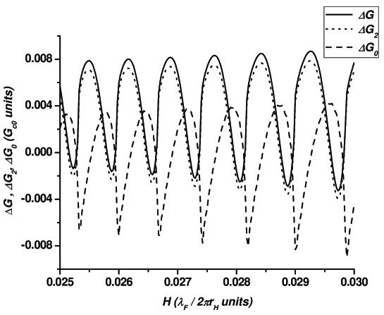
Figure 2: Oscillatory part of the conductance for a defect placed on the contact axis, $\rho_{0}=0,$ $z_{0}=30\lambdabar_{\mathrm{F}}$. The full curve is a plot for Eq. (III), while the dotted curve shows the component $\Delta G_{2}$ for the semiclassical approximation, Eq. (29), and the dashed curve shows the component $\Delta G_{0}$, Eq. (25). The constant of electron-defect interaction is taken as $\widetilde{g}=0.5.$ The field scale is given in units $\lambdabar_{\mathrm{F}}/r_{H}=(e\hbar/p_{\mathrm{F}}^{2}c)H$.

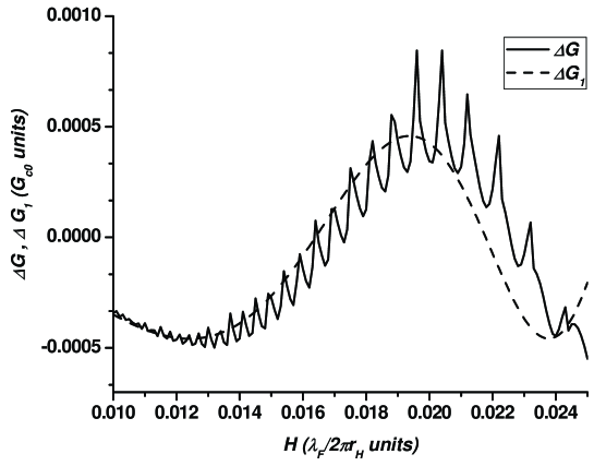
Figure 3: Oscillatory part of the conductance of a tunnelling point contact with a single defect placed at $\rho_{0}=50\lambdabar_{\mathrm{F}},$ $z_{0}=30\lambdabar_{\mathrm{F}}.$ The full curve is a plot for Eq. (III), while the dashed curve shows the component $\Delta G_{1}$ for the semiclassical approximation, Eq. (26). The field scale is given in units $\lambdabar_{\mathrm{F}}/r_{H}=(e\hbar/p_{\mathrm{F}}^{2}c)H$; $\widetilde{g}=0.5$.

For magnetic fields that are not too high one typically has a large number of Landau levels, $n_{\max}(\varepsilon_{\mathrm{F}})\approx\varepsilon_{\mathrm{F}}/\hbar\Omega=\left(a_{H}/\sqrt{2}\lambdabar_{\mathrm{F}}\right)^{2}\gg 1$, in which case the semiclassical approximation can be used. Some details of the calculations are presented in the Appendix. The asymptotic form of the expression for the conductance Eq. (III) can be written as a sum of four terms

$$G(H)=G_{c0}+\Delta G_{0}+\Delta G_{1}+\Delta G_{2}.$$ (23)

In leading approximation in the small parameter $\hbar\Omega/\varepsilon_{\mathrm{F}}$ the conductance (22) does not depend on the magnetic field

$$G_{c0}=\frac{4e^{2}}{9\pi\hbar}T(p_{\mathrm{F}})\left(\frac{p_{\mathrm{F}}a}{\hbar}\right)^{4},$$ (24)

where $T(p_{\mathrm{F}})=\left(\hbar p_{\mathrm{F}}/m^{\ast}U\right)^{2}\ll 1$ is the transmission coefficient of the tunnel junction. There is an oscillatory contribution $\Delta G_{0}$ to the conductance that originates from the step-wise dependence of the number of states $N(\varepsilon_{\mathrm{F}})$ on the magnetic field, and the conductance undergoes oscillations having the periodicity of the de Haas-van Alphen effect,

$$\Delta G_{0}=\frac{9}{2}G_{c0}\left(\frac{\lambdabar_{\mathrm{F}}}{a_{H}}\right)^{3}\sum\limits_{k=1}^{\infty}\frac{\left(-1\right)^{k}}{k^{3/2}}\sin\left(\pi k\frac{a_{H}^{2}}{\lambdabar_{\mathrm{F}}^{2}}-\frac{\pi}{4}\right).$$ (25)

The other two terms in Eq. (23), $\Delta G_{1}$ and $\Delta G_{2}$, result from the electron scattering on the defect.

Using the results presented in the Appendix, Eq. (A5), we find for the first oscillation,

$$\Delta G_{1}(H,\mathbf{r}_{0})=-G_{c0}\widetilde{g}\frac{z_{0}^{2}\lambdabar_{\mathrm{F}}^{2}}{r_{0}^{4}}\sin\left(\frac{2p_{\mathrm{F}}r_{0}}{\hbar}-2\pi\frac{\Phi}{\Phi_{0}}\right).$$ (26)

where $\widetilde{g}=3gm^{\ast}p_{\mathrm{F}}/4\pi\hbar^{3}$ is a dimensionless constant representing the defect scattering strength, and $\Phi_{0}=2\pi\hbar c/e$ is the flux quantum. The flux,

$$\Phi=HS_{\mathrm{pr}},$$ (27)

is given by the field lines penetrating the area of the projection $S_{\mathrm{pr}}=2S_{\mathrm{seg}}$ on the plane $z=0$ of the trajectory of the electron moving from the contact to the defect and back (see, Fig. 1),

$$S_{\mathrm{seg}}=r^{2}\left(\theta_{\mathrm{st}}-\sin 2\theta_{\mathrm{st}}\right).$$ (28)

$S_{\mathrm{seg}}$ is the area of the segment formed by the chord of length $\rho_{0}$ and the arc of radius $r=r_{H}\sin\theta_{\mathrm{st}}$, with $\theta_{\mathrm{st}}$ is the angle between the vector $\mathbf{r}_{0}$ and $z$-axis, $\sin\theta_{\mathrm{st}}=\rho_{0}/r_{0},$ $r_{H}=cp_{\mathrm{F}}/eH.$ The oscillation $\Delta G_{1}$ disappears when the defect sits on the contact axis, $\rho_{0}=0.$ Note that for $H\rightarrow 0$ Eq. (26) reduces to the expression obtained before Avotina1 for the point-contact conductance in the presence of a defect.

An analytic expression for the last term $\Delta G_{2}(H,\mathbf{r}_{0})$ in Eq. (23) can be written by use of Eq. (A8) as

$$\Delta G_{2}(H,\rho_{0}=0,z_{0})=G_{c0}\widetilde{g}\left(\frac{\lambdabar_{\mathrm{F}}}{a_{H}}\right)^{3}\times$$ (29)

$$\left\{\sum\limits_{k=\left[z_{0}/2\pi r_{H}\right]}^{\infty}\left(-1\right)^{k}\frac{1}{k^{3/2}}\cos\left(\frac{p_{\mathrm{F}}r_{0}}{\hbar}+\pi k\frac{a_{H}^{2}}{\lambdabar_{\mathrm{F}}^{2}}+\frac{z_{0}^{2}}{4\pi ka_{H}^{2}}\right)\right.+$$

$$\frac{z_{0}^{2}\sqrt{2}}{a_{H}^{2}}\left(\frac{\lambdabar_{\mathrm{F}}}{a_{H}}\right)\sum\limits_{k,k^{\prime}=\left[z_{0}/2\pi r_{H}\right]}^{\infty}\left(-1\right)^{k+k^{\prime}}\frac{1}{\left(kk^{\prime}\right)^{3/2}}\times$$

$$\left.\sin\left(\pi k\frac{a_{H}^{2}}{\lambdabar_{\mathrm{F}}^{2}}+\frac{z_{0}^{2}}{4\pi ka_{H}^{2}}\right)\cos\left(\pi k^{\prime}\frac{a_{H}^{2}}{\lambdabar_{\mathrm{F}}^{2}}+\frac{z_{0}^{2}}{4\pi k^{\prime}a_{H}^{2}}\right)\right\}.$$

As a consequence of the decreasing amplitudes of the summands with $k$ and $k^{\prime}$ the main contribution to the conductance oscillations results from the first term in the braces, with $k=\left[z_{0}/2\pi r_{H}\right]$. Comparing the dependence $G(H)$ that is obtained from Eq.(III) with the asymptotic expressions Eq.(29) in Fig. 2, and Eq.(26) in Fig. 3, we observe the good agreement between the exact solution and results obtained in the framework of semiclassical approximation. This agreement allows us to explain the nature of the complicated oscillations of the conductance $G(H).$

IV Discussion

The de Haas-van Alphen effect and the Shubnikov-de Haas effect are quite different manifestations of the Landau quantization of the electron energy spectrum in a magnetic field. The de Haas-van Alphen effect is a thermodynamic property that results from singularities in the electron density of states while the Shubnikov-de Haas effect is a manifestation of the Landau quantization due to corrections in the electron scattering LAK ; Abrikosov . It is known that a calculation of the metallic conductivity in a strong magnetic field in the approximation of a constant mean free scattering time gives an incorrect answer for the amplitude of the oscillations Lifshits . The correct amplitude can be obtained when the quantization is taken into account in the collision term of the quantum kinetic equation Kosevich .

We have considered the limiting case when there is only one scatterer and found specific magneto-quantum oscillations, the amplitude of which depends on the position of the defect. In our system a few quantum effects manifest themselves at the same time: 1) the Landau quantization, 2) the quantum interference between the wave that is directly transmitted through the contact and the partial wave that is scattered by the contact and the defect, 3) the effect of the quantization of the magnetic flux. As a consequence the conductance $G(H)$, Eq.(III), is a complicated non-monotonous function of the magnetic field, see Figs. 2 and 3.

First of all, Landau quantization results in the oscillations $\Delta G_{0}(H)$ of Eq.(25), having the usual period of the Shubnikov-de Haas (or de Haas-van Alphen) oscillations. From the point of view of the first paragraph of this section, the oscillatory part of the conductance (25) is not a manifestation of the Shubnikov-de Haas effect but it is due to the oscillations in the number of states that modify the conductivity of the tunnel junction.

At $H=0$ the quantum interference between partial electron waves (the directly transmitted wave and the wave scattered by the defect and reflected back to the contact) leads to an oscillatory dependence of the conductance as a function of the position of the defect Avotina1 and the period of this oscillation can be found from the phase shift $\Delta\phi=2p_{\mathrm{F}}r_{0}/\hbar$ between the two partial waves. Experimentally the oscillation can be observed as a function of the bias voltage, which changes the momentum of the incoming electrons. In a magnetic field the electron trajectory becomes curved (see trajectory 2 in Fig. 1) and the phase difference of two partial waves mentioned above is modified as,

$$\Delta\phi=2p_{\mathrm{F}}r_{0}/\hbar-2\pi\Phi/\Phi_{0},$$ (30)

where $\Phi$ is the magnetic flux through the projection $S_{\mathrm{pr}}$ (see Fig. 1) of the closed electron trajectory onto a plane perpendicular to the vector $\mathbf{H}$. For this reason the conductance undergoes oscillations with a period $\Phi/\Phi_{0}$. The sign in front of the second term in Eq. (30) is defined by the negative sign of the electron charge. The resulting oscillations in the conductance $\Delta G_{1}$ (26) have a nature similar to the Aharonov-Bohm effect and are related to the quantization of the magnetic flux through the area enclosed by the electron trajectory. In Fig. 3 the full expression for the oscillatory part $\Delta G(H)$ of the conductance (the second term in Eq. (III)) is compared with the semiclassical approximation $\Delta G_{1}(H,\rho_{0},z_{0})$, Eq (26). The long period oscillation is a manifestation of the flux quantization effect and is well reproduced by the semiclassical approximation. The short-period oscillations originate from the effect of the electron being focused by magnetic field.

In the absence of a magnetic field only those electrons that are scattered off the defect in the direction directly opposite to the incoming electrons can come back to the point-contact. When $H\neq 0$ the electrons move along a spiral trajectory (trajectory 1 in Fig. 1) and may come back to the contact after scattering under a finite angle to the initial direction. For example, if the defect is placed on the contact axis an electron moving from the contact with a momentum $p_{z}=p_{\mathrm{F}}$ along the magnetic field returns to the contact when the $z$-component of the momentum $p_{zk}=z_{0}m^{\ast}\Omega/2\pi k$, for integer $k$. For these orbits the time of the motion over a distance $z_{0}$ in the $z$ direction is a multiple of the cyclotron period $T_{H}=2\pi/\Omega$. Thus, after $k$ revolutions the electron returns to the contact axis at the point $z=0.$ The phase which the electron acquires along the spiral trajectory is composed of two parts, $\Delta\phi=\Delta\phi_{1}+\Delta\phi_{2}.$ The first, $\Delta\phi_{1}=p_{zk}z_{0}/\hbar$ is the ‘geometric’ phase accumulated by an electron with momentum $p_{zk}$ over the distance $z_{0}$. The second, $\Delta\phi_{2}=\pi k(eHr_{k}^{2}/c\hbar)$ is the phase acquired during $k$ rotations in the field $H,$ where $r_{k}=c\sqrt{p_{\mathrm{F}}^{2}-p_{zk}^{2}}/eH$ is the radius of the spiral trajectory. Substituting $p_{zk}$ and $r_{k}$ in the equation for $\Delta\phi$ we find

$$\Delta\phi=\pi ka_{H}^{2}/\lambdabar_{\mathrm{F}}^{2}+z_{0}^{2}/4\pi ka_{H}^{2}.$$ (31)

This is just the phase shift that defines the period of oscillation of the first term in the contribution $\Delta G_{2}$ (29) to the conductance. It describes a trajectory which is straight for the part from the contact to the defect and spirals back to the contact by $k$ windings. The second term in Eq. (29) corresponds to a trajectory consisting of helices in the forward and reverse paths, with $k$ and $k^{\prime}$ coils, respectively.

Note that, although the amplitude of the oscillation $\Delta G_{2}$ (29) is smaller by a factor $\hbar\Omega/\varepsilon_{\mathrm{F}}$ than the amplitude of the contribution $\Delta G_{1}$ (26), the first depends on the depth of the defect as $z_{0}^{-3/2}$ and $z_{0}^{-1}$ while $\Delta G_{1}\sim z_{0}^{-2}.$ The slower decreasing of the amplitude for $\Delta G_{2}$ is explained by the effect of focusing of the electrons in the magnetic field.

In a high magnetic field the selection of semiclassical trajectories that connect the contact and the defect is restricted by the quantization condition. The projection of the momentum $p_{z,n}$ (12) in the direction of the vector $\mathbf{H}$ is quantized and for a fixed quantum number $n$ $p_{z,n}$ depends on $H$. For increasing magnetic field the distance between the Landau levels, $\hbar\Omega$, increases and $p_{z,n}$ decreases until $\varepsilon_{n0}=\varepsilon_{\mathrm{F}}$. As a result, for sufficiently large $z_{0}$ each term in the conductance (III) corresponding to the set of quantum numbers $\left(n,n^{\prime}\right)$ undergoes one more oscillation. This is confirmed by the results presented in Fig. 2, in which the dependencies of the $\Delta G(H)$ (III) and the semiclassical asymptotic $\Delta G_{2}(H,\rho_{0}=0,z_{0})$ (29) are shown for a position of the defect on the contact axis $(\rho_{0}=0).$

In order to observe experimentally the predicted effects it is necessary to satisfy a few conditions: a) The distance between Landau levels $\hbar\Omega$ is larger then the temperature $k_{\mathrm{B}}T.$ This is the condition for observing effects of the quantization of the energy spectrum. b) The radius of electron trajectory, $r_{H}$, and the distance between the contact and the defect, $r_{0}$, are much smaller then the mean free path of the electrons for electron-phonon scattering. This condition is necessary for the realization of the almost ballistic electron kinetics (the scattering is caused only by a single defect) that has been considered. c) For the observation of the Aharonov-Bohm-type oscillations the position $\rho_{0}$ of the defect in the plane parallel to the interface must be smaller then $r_{H}$, i.e. the defect must be situated inside the ‘tube’ of electron trajectories passing through the contact. At the same time the inequality $\rho_{0}>a_{H}=\sqrt{r_{H}\lambdabar_{\mathrm{F}}}$ must hold in order that a magnetic flux quantum $\Phi_{0}$ is enclosed by the area of the closed trajectory. d) The distance $r_{0}$ should not be very large on the scale of the Fermi wave length, because in such case the amplitude of the quantum oscillations resulting from the electron scattering by the defect becomes small. Although these conditions restrict the possibilities for observing the oscillations severely, all conditions can be realized, e.g., in single crystals of semimetals (such as Bi, Sb and their ordered alloys) where the electron mean free path can be up to millimeters and the Fermi wave length $\lambda_{\mathrm{F}}\sim 10^{-8}$m. Also, as possible candidates for the observation of predicted oscillations one may consider the metals of the first group, the Fermi surface of which has small pockets with effective mass $m^{\ast}\simeq 10^{-2}\div 10^{-3}m_{0}$ LAK . For estimating the periods and amplitudes of the oscillations we shall use the characteristic values of the Fermi momentum $p_{\mathrm{F}}$ and effective (cyclotron) mass $m^{\ast}$ for the central cross-section of the electron ellipsoids of the Bi Fermi surface, $p_{\mathrm{F}}\simeq 0.6\cdot 10^{-26}$kg m/s and $m^{\ast}/m_{0}\simeq 0.008$ Fal . For such parameters the magnetic field of $H=0.03$ in units $\lambdabar_{\mathrm{F}}/r_{H}$ shown in Figs. (2), (3) corresponds to $H\simeq 0.1$T.

The amplitude of the conductance oscillations depends mainly on the constant of electron-defect interaction $g$ (16), which can be estimated using an effective electron scattering cross section $\sim$ $\lambda_{\mathrm{F}}^{2}.$ In the plots of Figs. 2 and 3 we used a typical value for the dimensionless constant $\widetilde{g}\sim 0.5$. The long-period oscillations (see Fig. 3) require a large $\rho_{0},$ the distance between the contact and the defect in the plane of interface, and their relative amplitude is of the order of $10^{-3}G_{c0}.$ The amplitude of short-period oscillations for such arrangement of the contact and the defect is small, $\sim 10^{-4}G_{c0}$, but it increases substantially and becomes $10^{-3}G_{c0}$ if the defect is situated at the contact axis (see Fig. 2). The amplitude of the oscillations (25) having de Haas-van Alphen period is proportional to the small parameter $\left(\hbar\Omega/\varepsilon_{\mathrm{F}}\right)^{3/2},$ which for $H\sim 0.1T$ is of the order of $\sim 10^{-3}G_{c0}.$ Comparing this to previous STS experiments Stipe , where signal-to-noise ratios of $5\cdot 10^{-4}$ (at 1 nA, 400 Hz sample frequency) have been achieved, it should be possible to observe the predicted conductance oscillations.

The predicted oscillations, Eqs. (26) and (29), are not periodic in $H$ nor in $1/H$. Their typical periods can be estimated as a difference $\Delta H$ between two nearest-neighbor maxima. For the short-period oscillations (29) we find

$$\left(\frac{\Delta H}{H}\right)_{SP}\simeq\frac{2\lambdabar_{\mathrm{F}}^{2}}{a_{H}^{2}}\left(1-\left(\frac{z_{0}\lambdabar_{\mathrm{F}}}{2\pi a_{H}^{2}}\right)^{2}\right)^{-1}$$ (32)

The period (32) depends on the position of the defect. It is larger than the period of de Haas-van Alphen oscillation, $\left(\Delta H/H\right)_{dHvA}\simeq 2\lambdabar_{\mathrm{F}}^{2}/a_{H}^{2}.$ Both of these periods are of the same order of magnitude as can be seen from Fig. 2. For a semimetal $\left(\Delta H\right)_{SP}\sim 10^{-2}$T in a field of $H\sim 0.1$T. The characteristic interval of the magnetic fields for the long-period oscillations is $\left(\Delta H/H\right)_{LP}\sim 0.1$T as can be seen from Fig. 3.

The experimental study of the magneto-quantum oscillations of the conductance of a tunnel point-contact considered in this paper may be used for a determination of the position of defects below a metal surface, similar to the current-voltage characteristics considered in Ref. Avotina1 . Although the dependence $G(H)$ with magnetic field is more complicated then the dependence $G(V)$ on the applied bias, in some cases such investigations may have advantages in comparison with the methos proposed in Avotina1 because with increasing voltage the inelastic mean free path of the electrons decreases, which restricts the use of voltage dependent oscillations.

One of the authors (Ye. S. A) is supported by the INTAS grant for Young Scientists (No 04-83-3750) and partly supported by grant of President of Ukraine (No. GP/P11/13) and one of the authors (Yu.A.K.) was supported by the NWO visitor’s grant.

V Appendix: Summation over quantum numbers in semiclassical approximation.

Here we illustrate the procedure for the calculations of the correction to the conductance due to the presence of the defect in the semiclassical approximation. At $n_{\max}(\varepsilon_{\mathrm{F}})\gg 1$ in the Eq. (III) the summation over discrete quantum numbers $n^{\prime}$ and $n^{\prime\prime}$  can be carried out using the Poisson summation formula. Let us consider the sum of the functions $\chi(\varepsilon_{\mathrm{F}},n,\mathbf{r}_{0})$ (20)

$$S=\sum\limits_{n=0}^{n_{\max}(\varepsilon_{\mathrm{F}})}\chi(\varepsilon_{\mathrm{F}},n,\mathbf{r}_{0})=S_{1}+S_{2}=$$ (A1)

$$\int\limits_{0}^{n_{\max}}dn\chi(\varepsilon_{\mathrm{F}},n,\mathbf{r}_{0})+\sum\limits_{k=-\infty,k\neq 0}^{\infty}\left(-1\right)^{k}\int\limits_{0}^{n_{\max}}dn\chi(\varepsilon_{\mathrm{F}},n,\mathbf{r}_{0})\,e^{2i\pi kn}.$$

By using the Tricomi asymptotic for the Laguerre polynomials at $n\gg 1$ Tricomi we find an expression for the first term $S_{1}$ in Eq. (A1) for fields that are not too high such that $n$ is large and $\rho_{0}/(2a_{H}\sqrt{\left(2n+1\right))}<1$,

$$S_{1}\simeq\sqrt{\frac{2}{\pi}}\int\limits_{0}^{n_{\max}}\frac{dn}{\sqrt{\left(2n+1\right)\sin 2\theta}}\cos\left[\left(2n+1\right)2\theta-\left(n+\frac{1}{2}\right)\left(2\theta-\sin 2\theta\right)\right]\times$$ (A2)

$$\exp\left(\frac{i}{\hbar}z_{0}\sqrt{2m^{\ast}\left(\varepsilon_{\mathrm{F}}-\hbar\Omega\left(n+\frac{1}{2}\right)\right)}\right),$$

where

$$\sin^{2}\theta=\frac{\rho_{0}^{2}}{4a_{H}^{2}\left(2n+1\right)}.$$ (A3)

For large $n$ the functions in the integrand of Eq. (A2) rapidly oscillate and $S_{1}$ can be calculated by the method of stationary phase points. As can be seen from Eq. (A3), for $n\sim n_{\max}\sim\varepsilon_{\mathrm{F}}/\hbar\Omega$ we have $\sin\theta\approx\rho_{0}/2r_{H}$, where $r_{H}=v_{\mathrm{F}}/\Omega$ is the radius of electron trajectory. For $\rho_{0}\ll r_{H}$ in Eq. (A2) we can make the approximations $n\theta\sim\rho_{0}/\lambda_{\mathrm{F}},$ $n\left(2\theta-\sin 2\theta\right)\sim\left(\rho_{0}/r_{H}\right)^{2}\left(\rho_{0}/\lambda_{\mathrm{F}}\right)$, and $(z_{0}/\hbar)\sqrt{2m^{\ast}\left(\varepsilon_{\mathrm{F}}-\hbar\Omega\left(n+\frac{1}{2}\right)\right)}\sim z_{0}/\lambda_{\mathrm{F}}.$ If $\rho_{0}$ or $z_{0}$ is much larger than $\lambda_{\mathrm{F}},$ and the second term under the cosine in Eq. (A2) is of order unity so that it can be considered as a slowly varying function, the stationary phase point of the integral (A2) is given by,

$$n_{\mathrm{st}}\simeq\frac{\varepsilon_{\mathrm{F}}}{\hbar\Omega}\frac{\rho_{0}^{2}}{r_{0}^{2}},$$ (A4)

where $r_{0}=\sqrt{\rho_{0}^{2}+z_{0}^{2}}$ is the distance between the point contact and the defect. The asymptotic value of $S_{1}$ takes the form

$$S_{1}\simeq-\frac{ir_{H}z_{0}}{r_{0}^{2}}\exp\left(\frac{i}{\hbar}p_{\mathrm{F}}r_{0}-i\pi\frac{\Phi}{\Phi_{0}}\right),$$ (A5)

where $\Phi$ is given by Eq.(27).

The second term $S_{2}$ in the sum (A1) describes an oscillation of a different type. We consider this term for a defect position with $\rho_{0}=0.$ Replacing the integration over $n$ by the integration over momentum along the magnetic field $p_{n}=\sqrt{2m^{\ast}\left(\varepsilon_{\mathrm{F}}-\hbar\Omega\left(n+\frac{1}{2}\right)\right)}$ we rewrite the second term in Eq. (A1) in the form

$$S_{2}\simeq\sum\limits_{k=-\infty,k\neq 0}^{\infty}\left(-1\right)^{k}\int\limits_{0}^{\sqrt{2m^{\ast}\varepsilon_{\mathrm{F}}}}\frac{p_{n}dp_{n}}{m^{\ast}\hbar\Omega}\exp\left[2\pi ki\left(\frac{\varepsilon_{\mathrm{F}}}{\hbar\Omega}-\frac{p_{n}^{2}}{2m^{\ast}\hbar\Omega}\right)+\frac{i}{\hbar}p_{n}z_{0}\right].$$ (A6)

The stationary phase points $p_{n}=p_{\mathrm{st}}$ of the integrals (A6) are

$$p_{\mathrm{st}}=\frac{z_{0}m^{\ast}\Omega}{2\pi k}.$$ (A7)

Note that the stationary phase point (A7) exists if $k>0$ and $z_{0}\leq 2\pi k\,r_{H}.$ The momenta (A7) have a clear physical meaning: The time $t=z_{0}m^{\ast}/$ $p_{\mathrm{st}}$ of the classical motion of electron from the contact to the defect is an integer multiple of the period $T_{H}=2\pi/\Omega$ of the motion in the field $H,$ $t=kT_{H}.$ This is the same condition as is applicable for longitudinal electron focusing Sharvin , in which case the electrons move across a thin film from a contact on one side to a contact on the opposite surface and the magnetic field is directed along the line connecting the contacts. The asymptotic expression for $S_{2}$ (A6) is given by,

$$S_{2}\simeq\frac{z_{0}}{2\pi a_{H}}\sum\limits_{k=\left[z_{0}/2\pi r_{H}\right]}^{\infty}\left(-1\right)^{k}\frac{1}{k^{3/2}}\exp\left(\pi ki\frac{a_{H}^{2}}{\lambdabar_{\mathrm{F}}^{2}}+\frac{iz_{0}^{2}}{4\pi ka_{H}^{2}}\right),$$ (A8)

where $\left[x\right]$ is the integer part of the number $x.$

References

- (1) B. Ludoph, M.H. Devoret, D. Esteve, C. Urbina and J.M. van Ruitenbeek, Phys. Rev. Lett., 82, 1530, (1999).
- (2) C. Untiedt, G. Rubio Bollinger, S. Vieira, and N. Agraït, Phys. Rev. B, 62, 9962 (2000).
- (3) B. Ludoph and J. M. van Ruitenbeek, Phys. Rev. B, 61, 2273 (2000).
- (4) A. Halbritter, Sz. Csonka, G. Mihály, O. I. Shklyarevskii, S. Speller, and H. van Kempen, Phys. Rev. B, 69, 121411 (2004).
- (5) Ye. S. Avotina, Yu. A. Kolesnichenko, A.N. Omelyanchouk, A.F. Otte, and J.M. van Ruitenbeek, Phys. Rev. B 71, 115430 (2005).
- (6) A. Namiranian, Yu. A. Kolesnichenko, and A. N. Omelyanchouk, Phys. Rev. B, 61, 16796 (2000).
- (7) Ye. S. Avotina, and Yu. A. Kolesnichenko, Fiz. Nizk. Temp., 30, 209 (2004) [Low Temp. Phys., 30, 153 (2004)].
- (8) Ye. S. Avotina, A. Namiranian, and Yu. A. Kolesnichenko, Phys. Rev. B, 70, 075908 (2004).
- (9) Ye. S. Avotina, Yu. A. Kolesnichenko, A.F. Otte, and J.M. van Ruitenbeek, Phys. Rev. B, 74, 085411 (2006).
- (10) N. Quaas, PhD thesis, Göttingen University (2003); N. Quaas, M. Wenderoth, A. Weismann, R.G. Ulbrich and K. Schönhammer, Phys. Rev. B 69, 201103(R) (2004).
- (11) I.M. Lifshits, M.Ya. Azbel’, and M.I. Kaganov, ’Electron theory of metals’, New York, Colsultants Bureau (1973).
- (12) A. A. Abrikosov, ’Fundamentals of the theory of metals’, North Holland, 1988.
- (13) E. N. Bogachek, I. O. Kulik and R. I. Shekhter, Zh. Exp. Teor. Fiz.,92, 730 (1987). [Sov. Phys., JETP, 65, 411 (1987)].
- (14) E. N. Bogachek, I. O. Kulik and R. I. Shekhter, Solid State Commun., 56, 999 (1985).
- (15) E. N. Bogachek, and R. I. Shekhter, Fiz. Nizk. Temp., 14, 810 (1988) [Sov. J. Low Temp. Phys., 14, 445 (1988)].
- (16) N. N. Gribov, O. I. Shklyarevskii, E. I. Ass, and V. V. Andrievskii, Fiz. Nizk. Temp., 13, 642 (1987) [Sov. J. Low Temp. Phys., 13, 363 (1987)].
- (17) C. Kittel, Quantun Theory of Solids, John WileySons Inc., New York-London (1963).
- (18) I. O. Kulik, Yu. N. Mitsai, and A. N. Omelyanchouk, Zh. Exp. Teor. Fiz., 63, 1051 (1974).
- (19) L. D. Landau and E. M. Lifshits, Quantum Mechanics, Pergamon, Oxford (1977).
- (20) I. F. Itskovich and R. I. Shekhter, Fiz. Nizk. Temp., 11, 373 (1985) [Sov. J. Low Temp. Phys., 11, 202 (1985)].
- (21) Yu.V. Sharvin, Zh. Exp. Teor. Fiz., 48, 984 (1965).
- (22) I.M. Lifshits, Zh. Exp. Teor. Fiz., 32, 1509 (1957).
- (23) A.M. Kosevich, and V.V. Andreev, Zh. Exp. Teor. Fiz., 38, 882 (1960).
- (24) H. Bateman, A. Erdelyi, Higher Transcendental Functions, V.2, Mc Graw-Hill Book Company, INC (1953).
- (25) L. A. Fal’kovskii, Physics-Uspekhi, 11, 1 (1968).
- (26) B. C. Stipe, M. A. Rezaei, and W. Ho, Rev. Sci. Instr. 70, 137 (1999).