Network Analysis of the State Space of Discrete Dynamical Systems

Abstract

We study networks representing the dynamics of elementary 1-d cellular automata (CA) on finite lattices. We analyze scaling behaviors of both local and global network properties as a function of system size. The scaling of the largest node in-degree is obtained analytically for a variety of CA including rules 22, 54 and 110. We further define the path diversity as a global network measure. The co-appearance of non-trivial scaling in both hub size and path diversity separates simple dynamics from the more complex behaviors typically found in Wolfram’s Class IV and some Class III CA.

As physical theories widen into the biological and social realms, the problem of characterizing complex dynamical systems becomes increasingly important. Even elementary systems, such as cellular automata (CA), originally proposed by von Neumann von Neuman (1966), often exhibit dynamical patterns that pose conceptual challenges and serve as test-beds for techniques to study more realistic phenomena. To date, attempts to classify the behavior of dynamical systems such as CA have been based on various definitions of complexity and have largely focused on patterns generated in space and time (see, e.g., Ref. Grassberger (1986a); Huberman and Hogg (1986); Badii and Politi (1997); Bialek et al. (2001); Feldman and Crutchfield (1998)). Here we take a different approach, focusing on statistical properties of state space networks.

The trajectories of a discrete dynamical system form a directed network in state space, wherein each node, representing a state, is the source of a link that points to its dynamical successor Wuensche and Lesser (1992). For deterministic systems, each node has a single outgoing link (each out-degree is equal to 1). For irreversible systems, states may have different numbers of pre-images and thus different in-degrees. In this paper we present analytical and numerical studies of state space networks of various one-dimensional CA. This network perspective reveals previously unrecognized scaling behaviors and suggests a new measure of an aspect of complexity that we term “path diversity.” Since the CA we study are known to produce a wide variety of different dynamical behaviors, our results are relevant for understanding discrete dynamical systems in general.

We examine 1-d binary CA with nearest neighbor interactions and periodic boundary conditions. Wolfram put these CA into four complexity classes Wolfram (1984) based on the qualitative appearance of spatio-temporal patterns produced from random initial conditions for large lattice size $L$. The four classes are: (I) the system almost always evolves quickly to a unique fixed point; (II) it almost always evolves quickly to one of many attractors with a small period; (III) it generates seemingly random patterns with small-scale structures; (IV) it shows a mixture of order and randomness with long characteristic times. One class IV CA, Rule 110 (defined below), has been shown to emulate a universal Turing machine Cook (2004). One shortcoming of this classification is that the border between classes III and IV is ill-defined. In fact, the classification of some rules (such as rule 54) is still disputed, and misclassifications can happen due to e.g. subtle and slow dynamics hidden beneath clear chaotic behavior. Examples include rule 18, where annihilating random walks are embedded in a random pattern with small-scale structure Grassberger (1983), and rule 22 which shows random patterns with slow but (highly) statistically significant decrease of entropy with time and with $L$ Grassberger (1986b). Other classifications have been suggested, but a definitive criterion for complex dynamics has not yet emerged Cullik II et al. (1990); Gutowitz (1990); Dhar et al. (1995).

In the present Letter we report numerical and analytical results showing that class IV and some class III CA exhibit highly heterogeneous state space networks, unlike the networks corresponding to the simple CA in class I and II. The heterogeneity is reflected in local properties, including broad in-degree distributions and finite-size scaling of the largest in-degree. We show, however, that this type of local heterogeneity can also occur in CA with simple dynamics. On the other hand, a global measure, termed the path diversity, by itself cannot distinguish simple from complex CA either. However, it tends to show trivial behavior in simple CA where the local measures are non-trivial. In fact, the complex rules show non-trivial scaling behavior in both the local measures and in the path diversity. On the basis of these observations, we speculate that network heterogeneity at multiple levels may be a generic property of the state space of complex dynamical systems.

Let $R$ denote the CA rule. The binary value $s^{t+1}_{i}$ of site $i$ at time $t+1$ is set equal to $R(s^{t}_{i-1}s^{t}_{i}s^{t}_{i+1})$ evaluated at the previous time $t$. We use periodic boundary conditions so that spatial indices are taken modulo $L$. To label the CA rules, we use Wolfram’s scheme that identifies each rule with the number $R(000)+2R(001)+2^{2}R(010)+2^{3}R(011)+2^{4}R(100)+2^{5}R(101)+2^{6}R(110)+2^{7}R(111)$. Hence, for example, Rule 18 is the one for which $R(100)=1$ and $R(001)=1$ and $R(s_{1}s_{2}s_{3})=0$ for all other triples.

A binary CA of size $L$ has $N=2^{L}$ different states ${\bf S}^{(a)}=(s_{0}^{(a)}\ldots s_{L-1}^{(a)}),\;a=0,\ldots,N-1$. These may be viewed as the nodes of a directed network, where a link from ${\bf S}^{(a)}$ to ${\bf S}^{(b)}$ indicates that $R$ maps ${\bf S}^{(a)}$ to ${\bf S}^{(b)}$. When such a link exists, we say that ${\bf S}^{(a)}$ is a pre-image of ${\bf S}^{(b)}$ and the number of pre-images of ${\bf S}^{(b)}$ is its in-degree $k({\bf S}^{(b)})$. The network typically consists of disconnected clusters, each containing transient states and a recurrent dynamical attractor. Garden of Eden (GoE) states are transient states with zero in-degree. Pictures of some state space clusters are shown in Fig. 1; for more, see Wuensche and Lesser (1992).

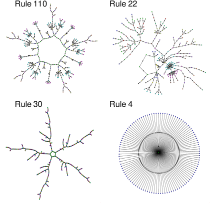
Figure 1: One connected cluster out of each state space network for different CA, plotted with the program ‘Pajek’ (vlado.fmf.uni-lj.si/pub/networks/pajek/). All arrows point from leaves towards the center. Sizes are $L=10$ to 13. For Rule 4, the network heterogeneity resides entirely in the size distribution of the different clusters making the state space network.

These state space networks can be analyzed by a variety of statistical measures – e.g. their degree distribution, clustering coefficients, etc. Newman (2003); Albert and Barabasi (2002). Many real-world networks (e.g. regulatory networks Albert (2005), the world-wide web Barabasi et al. (2000), and earthquakes Baiesi and Paczuski (2004)) differ markedly from random graphs (where degree distributions are Poissonian and clustering is absent), displaying “fat-tailed” or even scale-free degree distributions. In the following we show similar results also for state space networks.

Fig. 2 demonstrates that several CA networks exhibit clean scaling for a particular local property, the in-degree of the largest hub, $k_{max}\sim N^{\nu}$. Scaling sets in already for rather small lattices and holds also for the second, third, etc., largest hub (data not shown). The rules shown in Fig. 2 were chosen to cover the entire spectrum of known behaviors for 1-d elementary CA.

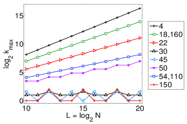
Figure 2: (color on-line) The largest in-degree $k_{max}$ as a function of $N=2^{L}$. Except for class III rules 30, 45 and 150, all CA shown here exhibit clear scaling of the largest hub size $k_{max}$ with the total number of nodes in the network, $N$. Rule 160 is class I, 4 and 50 are class II, and 110 is class IV. Rules 18, 22, and 54 are between III and IV, as they have large structures masked by small-scale chaos (18, 22) or structures on intermediate scales (54). The analytic values of $\nu$ are $0.8114,0.6942,0.5515,0.4057,0.3471,0.4057$ and $0.6942$ for rules 4, 18, 22, 50, 54, 110 and 160. These values are in perfect agreement with the numerical results.

This scaling, including the value of $\nu$, can be derived exactly, provided one knows the structure of the hub state ${\cal H}$. The latter can be guessed easily for all CA shown in Fig. 2, while it is less obvious for others. For all elementary CA, the hub state is either periodic or – if the period does not match the lattice size – periodic with a few defects.

For rule 18, e.g., one finds numerically that ${\cal H}=(00\cdots 00)$ for all $L$. According to the definition of CA 18 given above, all sequences that do not contain 001 or 100 as substrings are pre-images of $\cal H$.

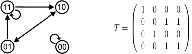
Figure 3: Walks on the graph shown on the left generate all pre-images of the hub state ${\cal H}$ for rule 18. Each step corresponds to an element of the matrix ${\bf T}$ shown on the right, with rows and columns labeled in the order $00,01,10,11$.

The number of distinct strings of length $\ell$ without ‘001’ or ‘100’ is equal to the number of walks with $\ell-2$ steps on the graph shown in Fig. 3. The number of periodic strings of length $L$ is then given by ${\rm Tr}{\bf T}^{L}\approx N^{\log_{2}\lambda_{1}}$, where ${\bf T}$ is the matrix shown on the right of Fig. 3, and $\lambda_{1}$ is its largest eigenvalue. This gives $k_{max}\sim N^{\nu}$ with $\nu=\log_{2}\lambda_{1}=0.6942$, in perfect agreement with the numerical results.

Similar analytic arguments hold for all the other CA that exhibit scaling in Fig. 2. When the hub state contains both ‘0’s and ‘1’s, one has to introduce two transfer matrices ${\bf T}^{(0)}$ and ${\bf T}^{(1)}$ where $T^{(s)}$ maps each pair $s_{i-1}^{t}s_{i}^{t}$ onto the pair $s_{i}^{t}s_{i+1}^{t}$, iff $s_{i}^{t+1}\equiv R(s_{i-1}^{t}s_{i}^{t}s_{i+1}^{t})=s$. The labeling of rows and columns is as in Fig. 3. The in-degree of any state ${\bf S}$ is then

$$k({\bf S})={\rm Tr}({\bf T}^{(s_{0})}\cdots{\bf T}^{(s_{L-1})})~{}.$$ (1)

The resulting exponents $\nu$ are cited in the caption for Fig. 2. The same scaling (with the same exponents) holds also for the second, third, etc. largest hub.

Another interesting property of rules giving large hubs is the scaling of the in-degree distribution function $P(k)$ with system size. Fig. 4 shows the data collapse for Rules 4, 22, and 110 found using the multiscaling ansatz Lise and Paczuski (2001)

$$\log P(k)=\log N\;f(\log k/\log N)\;.$$ (2)

It is significantly better than the usual finite size power-law scaling, which would produce straight lines in Fig. 4. To decide whether the apparent curvature is a finite size effect or a true indication of multiscaling is in general not easy, but it can be done analytically for the simple CA, Rule 4.

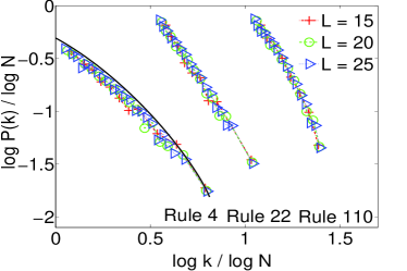
Figure 4: (color on-line) In-degree distribution functions collapsed for simple and complex rules using a multiscaling ansatz for rules 4, 22, and 110 for different system sizes. The black solid line is Eq. (7). The distributions were shifted by 0.5 units each for clarity. Rule 22 is consistent with a power law $P(k)\sim k^{-\gamma}$ with $\gamma\approx 2.8$.

For Rule 4, the sequence $\dots 11\ldots$ has no pre-image and the sequence $\ldots 1\ldots$ has the unique pre-image $\ldots 010\ldots$. ${\bf T}^{(1)}$ can then be written as ${\bf e}_{2}^{\top}{\bf e}_{3}$, where ${\bf e}_{2}=(0,1,0,0)$ and ${\bf e}_{3}=(0,0,1,0)$. The in-degree of any state ${\bf S}$ can then be expressed as

$$\prod_{i}w(m_{i})=\prod_{i}{\bf e}_{3}\,[{\bf T}^{(0)}]^{m_{i}}\,{\bf e}_{2}^{\top},$$ (3)

where

$${\bf T}^{(0)}=\left(\begin{array}[]{cccc}1&1&0&0\\ 0&0&0&1\\ 1&1&0&0\\ 0&0&1&1\end{array}\right)\;,$$ (4)

the product runs over all ‘1’s in ${\bf S}$, and $m_{i}$ is the number of ‘0’s following the $i$th ‘1’ in ${\bf S}$.

For large $m$ we have $w(m)\approx a\lambda^{m}$, where $\lambda=1.75488$ is the largest eigenvalue of ${\bf T}^{(0)}$ and $a=0.234487=({\bf e}_{2}\cdot{\bf u})({\bf v}\cdot{\bf e}_{3})$, ${\bf u}$ and ${\bf v}$ being the right and left eigenvectors corresponding to $\lambda$, normalized to ${\bf v}\cdot{\bf u}=1$. Any state containing $n$ isolated 1s will then have an in-degree $k_{n}\approx\prod_{i=1}^{n}a\lambda^{m_{i}}=a^{n}\lambda^{L-n}$. Although occurrences of small $m_{i}$ can only be neglected for $n\ll L$, we find empirically that this formula reflects the qualitative behavior for larger $n$. To find $P(k)$, we now need to find $\Omega(n)$, the number of states with $n$ isolated 1s and no pairs ‘11’, and transform its dependence on $n$ into a dependence on $k$. On a periodic lattice of length $L$, one has $\Omega(n)=C(L-n,n)+C(L-n-1,n-1)$, where $C(\ell,m)=\ell!/[m!(\ell-m)!]$. To obtain an approximation for $P(k)$ we first invert the above relation between $k_{n}$ and $n$, giving $n(k)=(L\ln\lambda-\ln k)/[\ln(\lambda/a)]$, then use $P(k)\approx 2^{-L}\Omega(n)|dn/dk|$.

The scaling ansatz shown in Fig. 4 is indeed recovered by this approximation. To see this, we define

$$x\equiv\ln k/\ln N,\qquad y\equiv\ln P(k)/\ln N~{}.$$ (5)

With this choice, we have

$$\frac{n}{L}=\frac{\ln\lambda-x\ln 2}{\ln(\lambda/a)}$$ (6)

Neglecting a term $\ln\ln(\lambda/a)/(L\ln 2)$ in $y$, using Stirling’s formula, and taking the large $L$ limit of $\ln[\Omega(n)]/L$ for fixed $x$, we get

$$y\approx-1-x+\log_{2}\left[\frac{(1-\epsilon)^{1-\epsilon}}{\epsilon^{\epsilon}(1-2\epsilon)^{1-2\epsilon}}\right].$$ (7)

Here $\epsilon\equiv n/L$ is a function of $x$ through Eq. (6). Eq. (7) is shown as a solid line in Fig. 4. The curvature of this line clearly indicates that no substantial range exists over which the distribution is a power law. Using a Fourier method based on recursion relations, we have also determined numerically the exact distribution for $L=10,000$. It shows slightly enhanced curvature for small $x$, and is for large $x$ in excellent agreement with the above approximation. Hence we conclude that the apparent curvature seen in Fig. 4 for Rules 4 and 110, is not simply a finite size effect but more likely an indication of multiscaling.

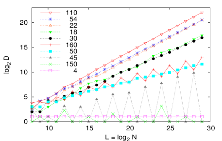
Figure 5: (color on-line) The path diversity $\cal D$ of different CA. Straight lines indicate scaling ${\cal D}\sim N^{\delta}$. Fitted values of $\delta$ are $0.88,0.88,0.85,0.75$ and 0.72 for rules 110, 22, 54, 18 and 30, respectively.

As Fig. 1 indicates, rule 4 does not exhibit heterogeneity beyond the single node level. All transients have length 1, all attractors are simple fixed points, and the only ‘complex’ aspect is the broad in-degree distribution of the latter. Clearly, the in-degree distribution of any set of nodes, being a strictly local construct, cannot by itself distinguish complex CA from trivial ones. To make this distinction we introduce a new quantity, the path diversity ${\cal D}$. It measures fluctuations in the set of different paths connecting the GoE states to attractors. If one projects all attractor states into a single node, then the state space network of a CA becomes a rooted tree. Roughly, ${\cal D}$ counts the number of non-equivalent choices encountered by following each path from an attractor (root) to a GoE state (leaf). Path diversity bears resemblances to tree diversity Huberman and Hogg (1986) and topological depth Badii and Politi (1997).

We first define the path diversity ${\cal D}$ for each transient node: A GoE state has diversity one; a transient state with a single pre-image has the same diversity as its unique pre-image; and the diversity of a node with more than one incoming link is the sum of all distinct diversities of its pre-images plus one. Thus, if a node has e.g. in-degree 5 and three of its pre-images have diversity 2, one has diversity 6, and the last has diversity 17, then that node’s diversity is $2+6+17+1=26$. Finally, the path diversity ${\cal D}$ of the entire CA is computed by joining all attractor states (in all disconnected components, if there are several) into one single “meta-state”, and applying the above scheme to the meta-state.

In Fig. 5, $\cal D$ is shown for several CA. It is sensitive to aspects of the network’s structure that are different from the node degree distribution. As a result, it clearly separates rules 4 (where ${\cal D}=2$ for all $L$) and 150 (where ${\cal D}$ seems to remain bounded) from other CA. The most interesting rules are those which show clear scaling ${\cal D}\sim N^{\delta}$ with $\delta$ close to 1, e.g. ${\delta}=0.88\pm 0.01$ (rules 22, 110), $0.85\pm 0.01$ (rule 54), $0.75\pm 0.04$ (rule 18), and $0.72\pm 0.03$ (rule 30). For the system sizes studied, rules 50 and 160 appear to show scaling with smaller $\delta$, though both would be classified as simple (classes I or II) by Wolfram. An analytical calculation of upper bounds on transient lengths shows, however, that ${\cal D}$ actually grows slower than any positive power of $N$ for rule 160, and we expect the same to hold for rule 50 given its similar numerics. The oscillations seen in Fig. 5 for some rules are due to the global constraint imposed by periodic boundary conditions. In the most extreme case, rule 45 has nontrivial transients for odd $L$ but none at all for even $L$.

In general, we neither expect that a single observable can reliably distinguish “complex” from other behavior, nor that a few discrete classes can do justice to the multifarious ways in which a system can display complexity. This is supported by our analysis. Neither the scaling of the hub sizes with system size (or the scaling of the in-degree distribution) nor the scaling of the path diversity can by itself distinguish between “simple” (Wolfram classes I and II) and “complex” (class IV and some class III) dynamics. Combined together, they fare already much better. We note also that within the class of CA for which $\cal D$ scales, those with largest ${\delta}$ (CA 110 and 22) are also those which have been considered most complex by previous authors Cook (2004); Grassberger (1986b).

In summary, we have studied networks formed by states of elementary 1-d CA on finite lattices. We find that some of them exhibit non-trivial scaling with system size, and this scaling behavior can be computed analytically in certain cases. Taken together, the the statistics of degree distribution (a local property) and path diversity (a global property) give a good indication of dynamical complexity. Including additional measures for network heterogeneity at intermediate scales could further refine this approach.

Part of this work was done at the Perimeter Institute for Theoretical Physics. J.E.S.S. and B.S. were supported by NSF Grant PHY-0417372 and the Institute for Biocomplexity and Informatics at the University of Calgary. W.N. was supported by NSF Grant CHE-0313618.

References

- von Neuman (1966) J. von Neuman, Theory of Self-Reproducing Automata (Univ. of Illinois Press, 1966).
- Grassberger (1986a) P. Grassberger, Int. J. Theor. Phys. 25, 907 (1986a).
- Huberman and Hogg (1986) B. Huberman and T. Hogg, Physica D 22, 376 (1986).
- Badii and Politi (1997) R. Badii and A. Politi, Phys. Rev. Lett. 78, 444 (1997).
- Bialek et al. (2001) W. Bialek et al., Physica A 302, 89 (2001).
- Feldman and Crutchfield (1998) D. Feldman and J. Crutchfield, Phys. Lett. A 238, 244 (1998).
- Wuensche and Lesser (1992) A. Wuensche and M. Lesser, The Global Dynamics of Cellular Automata (Addision-Wesley, 1992).
- Wolfram (1984) S. Wolfram, Physica D 10, 1 (1984).
- Cook (2004) M. Cook, Complex Syst. 15, 1 (2004).
- Grassberger (1983) P. Grassberger, Phys. Rev. A 28, 3666 (1983).
- Grassberger (1986b) P. Grassberger, J. Stat. Phys. 45, 27 (1986b).
- Cullik II et al. (1990) K. Cullik II et al., Physica D 45, 357 (1990).
- Gutowitz (1990) H. Gutowitz, Physica D 45, 136 (1990).
- Dhar et al. (1995) A. Dhar et al., Phys. Rev. E 51, 3032 (1995).
- Newman (2003) M. Newman, SIAM Rev. 45, 167 (2003).
- Albert and Barabasi (2002) R. Albert and A. Barabasi, Rev. Mod. Phys. 74, 47 (2002).
- Albert (2005) R. Albert, J. Cell Sci. 118, 4947 (2005).
- Barabasi et al. (2000) A. Barabasi et al., Physica A 281, 69 (2000).
- Baiesi and Paczuski (2004) M. Baiesi and M. Paczuski, Phys. Rev. E 69, 066106 (2004).
- Lise and Paczuski (2001) S. Lise and M. Paczuski, Phys. Rev. E 63, 036111 (2001).