I Introduction

A pivotal question of empiricism is the degree to which the results of an observation are expected. In ideal cases, either predictions based on these expectations remain valid in view of new measurements, or the expectations have to be changed. But this clear distinction is often blurred by uncertainties resulting from measurement errors, imprecision of model parameters, or the impossibility of extracting exact predictions from complicated models. Whether or not the problem at hand is a typical instance of a wider class of problems that are already understood is a question of statistical inference. In rare cases, the consequences of the expectations (or the model) can be derived analytically prior to observation. If this is not feasible, a widely used strategy is to construct a large number of “surrogates” eubank , or instances of a well-defined null model encapsulating the expectations, and to compare the actual observations to this artificial data.

Constructing surrogates is equivalent to simulating a statistical ensemble. In choosing weights for the ensemble of surrogates one often uses Occam’s razor—no outcome compatible with the null hypothesis should be preferred, and all such outcomes are equally likely. This is similar to Jaynes’ construction of statistical mechanics by maximizing Shannon entropy with physically meaningful constraints. Consequently, the numerical construction of surrogates often uses Monte Carlo methods schmitz-schreiber similar to those used in statistical mechanics.

This paper addresses properties of ensembles used as null models for complex networks. Predictions based on the null models fix expectations, and thereby determine whether or not deviations in the properties of an actual network are functionally or historically significant. While the numerical construction of surrogates of these ensembles has received attention in the recent literature maslov-sneppen ; milo04 ; chen05 , much less is known about analytic methods (see discussion below).

Nowadays networks attract enormous interest as representations of complex systems. They take various guises in biological, social, technological and physical contexts. The nodes designate distinct degrees of freedom (e.g agents, species, genes, magnetic concentrations in the solar photosphere, or earthquakes) and the links identify primary interactions or relationships between pairs of nodes (e.g. co-authorship, predator-prey relations, gene regulation, magnetic flux tubes, or seismic correlations). For examples see newman03 ; newmancollab ; aids ; gonorrhea ; foodweb ; stu ; mayapeterquake ; abc . The ubiquity of networks and their relatively easy visualization as graphs, together with notions of universality prevalent in the physics community, have driven speculations that the structure of networks can shed light on fundamental principles of social or biological organization, such as political behavior, ecosystem dynamics, brain function or the regulated homeostasis of organisms.

At the simplest level, networks are purely static entities, with each pair of distinct nodes connected by no more than one edge (or “link”). If, in addition, the interaction strength is disregarded (which often is a very useful simplification) the adjacency matrix $\cal M$ for the graph is a square (0,1) matrix. If $M_{ij}=1$ then an edge points from node $i$ to node $j$; if $M_{ij}=0$ then the edge is absent. Without self-interactions, $M_{ii}=0$. For undirected networks, the adjacency matrix is symmetric, $M_{ij}=M_{ji}$. The degree $k_{i}$ of node $i$ is then defined as the number of edges incident on it, $k_{i}=\sum_{j}M_{ji}$. Several reviews may be found in Refs. albert02 ; dorogo02 ; newman03 .

Section II defines more precisely the network ensembles (or null models) we consider in this paper. Our analytical methods focus on ensembles where the total number of links and nodes in the network is specified as well as the degrees of a small subset of nodes. These are called ensembles of “partially fixed degree sequence” (PFDS). Analytic predictions based on the PFDS ensembles can be compared with numerical results from a ‘rewiring’ algorithm for ensembles with fixed degree sequence (FDS), where the number of links attached to every node in the network is simultaneously specified. Section III mainly recalls previous results. We review Monte Carlo methods for sampling the FDS ensemble. Then we discuss how such null models can be used, and we conclude by recalling previous analytic approaches. Section IV discusses some results derived later in Section V, namely analytic estimates of the link linkelihood $p_{ij}$ (the linkelihood for a link to connect nodes $i$ and $j$). It uses them to make predictions for the average nearest neighbor degree $\langle k^{\prime}\rangle_{k}$ and for disassortativity. The calculation gives an excellent description of $\langle k^{\prime}\rangle_{k}$ for large $k$, e.g. for an Escherichia coli protein interaction network and an AS level map of the Internet. We also compute $\langle k^{\prime}\rangle_{k}$ analytically for the case where the degree distribution is a power law, using Eq. (1) given below. In that case, the naive approximation for $P(k,k^{\prime})$ would give divergent or ill-defined results.

Section V contains our main analytic results. In order to keep the notational clutter of this section to a minimum and to emphasize the intuitive nature of the results, most intermediate steps are moved to Appendix B. In the limit of large sparse networks with $L$ links and with the maximal degree much less than $L$, we find that the link likelihood depends only on $L$ and on the degrees $k$ and $k^{\prime}$ of the two nodes, and is given by

$$P(k,k^{\prime})\approx kk^{\prime}/(2L+kk^{\prime})\;.$$ (1)

This improves substantially over the widely used ‘naive’ approximation $P(k,k^{\prime})\approx kk^{\prime}/2L$. We also find that the disassortativity of the FDS ensembles corresponding to several real world networks is well-described by PFDS ensembles simultaneously fixing the degrees of two nodes at a time. Finally, we find an expression for the likelihood of a triangle, which factorizes in the same limit of large sparse networks (and when all three degrees are much larger than 1) to $P_{\Delta}(k_{1},k_{2},k_{3})=P(k_{1},k_{2})P(k_{1},k_{3})P(k_{2},k_{3})$, with $P(k,k^{\prime})$ given again by Eq. (1). The paper ends in section VI with a discussion and an outlook to further problems.

II Null Models for Networks

II.1 Erdös-Renyi (Undirected) Graphs

The simplest null hypothesis is that a given network is completely random, not even the number of links being specified. The only constraint is on the number of nodes, which is assumed to be $N$. Each pair of nodes may be joined with at most one link. Hence, the number of labelled undirected graphs with fixed $N$ is $Z_{0}(N)=2^{N(N-1)/2}$. This quantity is the number of ways undirected links may be placed in $\binom{N}{2}=N(N-1)/2$ possible positions. A statistical ensemble is obtained by assigning weights to each graph. The most natural choice is to weigh each graph with $L$ links by a factor $p^{L}$, where $p$ is the probability that two given nodes are connected by a link. This gives the average number of links as ${\bar{L}}=pN(N-1)/2$. The average degree of a node, i.e. the average number of links attached to it, is then ${\bar{k}}=2{\bar{L}}/N=p(N-1)$, and the degree distribution is binomial. In the limit of sparse networks, where $p\to 0$ for $N\to\infty$ such that $pN\to const.$, the degree distribution (or the probability $P(k)$ that a node has $k$ links) becomes Poissonian,

$$P(k)=\frac{{\bar{k}}^{k}\exp^{-\bar{k}}}{k!}\;.$$ (2)

While this ensemble can be viewed as a “grand canonical” version of the Erdös-Renyi ensemble bollobas since the particle fugacity is fixed, it is more customary to associate Erdös-Renyi graphs with a different ensemble where the total number $L$ of links is fixed, rather than just the average $\bar{L}$. Park and Newman refer to the ensemble with fixed $L$ as “canonical” park03 ; park04 , making an analogy between the number of links and the number of particles in traditional statistical mechanics. However, we shall refer to this ensemble, and ensembles with similar hard degree constraints, as microcanonical.

Excluding self-connections as well as multiple edges between any pair of nodes gives

$$Z_{1}(N,L)=\sum_{\left\{lg,N\right\}}^{\left\{L\right\}}1=\binom{\binom{N}{2}}{L}\qquad$$ (3)

distinct labelled, undirected graphs with fixed $N$ and $L$ footnote1 . The subscript “$\left\{lg,N\right\}$” indicates a sum over labelled graphs with $N$ nodes, while the superscript $\left\{L\right\}$ on the sum indicates, as in later formulae, the constraints on the edges. The subscript “1” on $Z$ indicates that $Z_{1}$ is the number of undirected graphs with one (global) hard constraint on the links, just as $Z_{0}(N)$ is the number of undirected graphs with zero constraints on the links.

With no further knowledge or constraints on the network, Occam’s razor suggests assigning equal weight to each labelled graph satisfying all the hard constraints. This corresponds exactly to the construction of microcanonical ensembles in statistical mechanics. For $Z_{1}$, each node has equal probability to be connected to any other node. It is easy to show burda05 that the distribution for the number of links attached to each node is again Poissonian for sparse networks with large $N$, where the grand canonical and microcanonical ensembles become equivalent.

In contrast, observations of real networks reveal fat-tailed degree distributions, which differ starkly from the situation where each node has equal likelihood to be connected to any other node. The most salient consequence is that the average degree $\bar{k}$ fails to characterize the connectivity of the nodes; in particular it cannot account for the dominant nodes or “hubs” with many links, which would not typically appear in the Erdös-Renyi ensemble.

II.2 Ensembles with Fixed Degree Sequences

As a result, attention has moved to ensembles that build additional information into the null hypothesis about the “distinguishability” or diversity of the nodes. Although many different and equally plausible ways to account for diversity can be imagined, to begin we focus on the most popular contemporary method. This uses the random ensemble of labelled graphs with fixed degree sequence (FDS) as the relevant null model. The complete degree sequence simultaneously fixes all the one-node properties for each member of the ensemble, without reference to their relationships (or links) in the network. Obviously, it is straightforward to obtain the degree sequence for any network, and there exist numerical methods to estimate characteristic properties of the corresponding FDS ensemble (see section III).

The microcanonical FDS ensemble is specified by assigning a specific degree (= number of links) to each node, $k_{i}$ for $i=1,...,N$, and giving equal weight to each graph with this degree sequence, while giving zero weight to all those graphs which have a different degree sequence. The null hypothesis for any observable pertinent to a specific graph ${\cal G}$ with adjacency matrix ${\cal M}_{\cal G}$ is then obtained by taking its expectation value in the FDS ensemble with the same degree sequence. For undirected graphs excluding self-interactions, the FDS partition sum is the number of symmetric (0,1) matrices with zeroes on the diagonal and with fixed marginal sums, which can be written according to our previous convention as

$$Z_{N}(N,L,k_{1},k_{2},...,k_{N-1})=\sum_{\left\{lg,N\right\}}^{\left\{k_{1}...,k_{N}\right\}}1\;.$$ (4)

with $k_{1}+k_{2}+...+k_{N}=2L$. For most networks of physical interest, $Z_{N}$ is astronomically large compared to one, but vanishingly small compared to $Z_{1}$. For instance, Chen et al. chen05 numerically estimate the number of $12\times 12$ (0,1) matrices with each row and column sum equal to 2 (and with no restrictions of symmetry or vanishing diagonal) to be $\approx 2.196\times 10^{16}$, which agrees well with the exact number found by Wang and Zhang wang98 . This number is much smaller than the number of all $12\times 12$ $(0,1)$ matrices with 24 ones, which is $\binom{12^{2}}{24}\approx 1.69\times 10^{29}$. Despite efforts by these and other mathematicians over decades bender ; wang98 , no well-developed, exact analytical approaches are known for these combinatorial problems, but advanced computational methods exist, as described in Section III.

II.3 Partially Fixed Degree Sequences

On the one hand, the difficulty of enumerating the number of graphs in the FDS ensemble suggests strong correlations in the graphs, since similar problems in systems lacking correlations can often be solved exactly. Indeed, the FDS ensemble makes very different predictions from the Erdös-Renyi (ER) ensemble, showing that taking into account some information about the nodes’ degrees is crucial.

On the other hand, it might be the case that not all the constraints in the FDS ensemble must be taken into account simultaneously. After all it is the simultaneous fixing of all the marginal sums in the matrix that makes the calculation of $Z_{N}$ difficult. Perhaps taking into account all the constraints, but not requiring them to be simultaneously enforced, is already sufficient to capture some nontrivial aspects of the FDS ensemble. If this is possible, then we must also identify which specific small subset of the nodes’ degrees gives the most reliable estimate of various expectation values in the FDS ensemble.

Here, we study ensembles where the degrees of a very small subset of the nodes are simultaneously fixed – the other degrees being arbitrary up to the constraint on the total number of links. We also demand that no more than one link may connect any two nodes in the network, and disallow self-connections. All graphs satisfying these constraints have equal weight. Those not satisfying these constraints are given zero weight. These ensembles can all be viewed as sub-ensembles of the ER ensemble. For each possible degree subset, we calculate the different partition functions corresponding to all possible subgraphs of a certain size. From these we can approximate expectation values of various quantities in the FDS ensemble.

In the following we shall always label the nodes such that the first $m$ degrees, $k_{1},...k_{m}$, are fixed. We call the resulting ensembles PFDS($m+1$): partially fixed degree sequence with $m+1$ constraints (the final constraint comes from fixing the number of links, $L$). Clearly, putting more constraints on the ensemble of labelled graphs diminishes its size until, when each and every edge is specified, the ensemble contains just one member - the real network ${\cal G}$ being studied. For ensembles with increasing numbers of link constraints this implies that $Z_{m+1}$ decreases monotonically with $m+1$, and

$$1\equiv Z_{\cal G}\ll Z_{N}(N,L,k_{1},k_{2},...,k_{N-1})\\ \ll Z_{m+1}(N,L,k_{1},...k_{m})\ll Z_{1}(N,L)\;\;,$$ (5)

for $1<m<N-1$.

We find that fixing only the degrees of the nodes participating in the small subgraph (e.g. link or triangle) under consideration, with explicit exclusion of self-connection and multiple-connections between any nodes, already gives a good approximation to the disassortativity (and to other properties) in the FDS ensemble. As noted above, this uses information about the whole degree sequence, but in each contribution corresponding to one specific (labelled) subgraph only part of this information is used.

The information stored in the degree sequence is most important when its distribution is very wide. Even for networks exhibiting broad degree distributions, such as protein interaction networks or autonomous system maps of the Internet, it is sufficient to fix the degrees of the node pairs directly involved (as well as the total number of links in the network) to obtain a good estimate of $\langle k^{\prime}\rangle_{k}$ and of the disassortativity. In order to estimate the number of triangles (i.e. the clustering), one has to fix the degrees of node triples. If we fix in addition the degrees of (some) hubs, this slightly improves the approximations. It is much easier to make analytical calculations for small $m$, with the smallest meaningful $m$ being the size of the subgraph being considered. Hence for link likelihoods and for $\langle k^{\prime}\rangle_{k}$ this minimum is $m=2$, while for triangle likelihoods it is $m=3$. By comparing analytic properties of the PFDS($m$) ensemble with numerical estimates of the FDS ensemble, we can assess to what extent the correlations in the PFDS ensembles resemble those in the FDS and in the ER ensembles.

To begin, we will focus in Section IV on the link likelihood, $p_{ij}$, which is the probability that a randomly chosen graph from the ensemble contains an edge from node $i$ to node $j$. From this microscopic quantity one can calculate the standard degree-degree correlations that are commonly compared with real-world networks to identify statistically significant features. Details of the calculation of $p_{ij}$ are deferred to Section V (and to Appendix B). There we will also treat the generalization to $m\geq 3$ which is needed in order to estimate the frequencies of higher order quantities such as motifs milo02 . As an example of a motif calculation, we include an estimate of the number of triangles.

III Background

III.1 Monte Carlo algorithms to estimate the FDS ensemble

As for many other problems where one wants to sample complex instances from some well-defined ensemble, here two basic strategies predominate: Markov chain Monte Carlo and sequential sampling Liu ; milo04 ; PERM . For the present case, the most obvious and popular Markov chain algorithm is the rewiring algorithm besag89 ; rao96 ; roberts00 ; cobb03 ; maslov-sneppen . We describe it here for directed graphs; the generalization to undirected graphs is immediate. We start by making an initial network with $N$ nodes, no self-connections, and the desired degree sequence, but without paying attention to multiple links between pairs of nodes footnote2 . The Monte Carlo algorithm proper consists of a sequence of moves, randomly chosen from a move set, which continues until equilibrium (i.e. uniformity of sampling) is reached with sufficient accuracy. A move is initiated by choosing randomly four different nodes $i,j,l$ and $m$ with $M_{ij}>0$ and $M_{lm}>0$. If either $M_{im}>0$ or $M_{lj}>0$, a null move is performed (the graph is left as it is). If neither of the pairs $\{i,m\}$ and $\{l,j\}$ were already connected by a link, $M_{ij}$ and $M_{lm}$ are each decreased by 1, while $M_{im}$ and $M_{lj}$ are increased by one. This corresponds to swapping one pair of links.

It can be shown easily that this algorithm eventually leads to a graph without multiple links (provided such a graph consistent with the fixed degree sequence exists). After this happens, the algorithm satisfies detailed balance (any sequence of moves is equally likely to be chosen as its reversed sequence) and is ergodic (each graph with the same degree sequences can be reached by a suitable move sequence.) As shown in rao96 , ergodicity is not strictly satisfied, but the few exceptions can be taken into account by including three-link exchanges in the move set.

Sequential sampling proceeds, in contrast, by repeatedly building a new graph from scratch. For this we start with an empty adjacency matrix and fill its entries randomly. In the simplest version, this is done without paying any attention to the degree sequence, to the absence of self loops, or to the exclusion of multiple links. Instead, the candidate graph is discarded if any of these constraints are violated. In this way the uniformity of the sampling is guaranteed, but the attrition (i.e. the chance to reach an illegal configuration) is overwhelming, rendering the algorithm useless. But there are more sophisticated options for sequential sampling. The most efficient algorithm studied in the literature chen05 uses detailed mathematical results for the structure of legal adjacency matrices Ryser57 to bias the matchings in a much more clever way.

III.2 Uses of null models

Statistically significant deviations between a null model and a real network point to organizing laws or historical accidents that are not accounted for by the null hypothesis. On the other hand, finding no statistically significant deviations would promote the belief that the entire structure of the network could be accounted for by the model, e.g. by the complete degree sequence in case of the FDS ensemble. This process of building null models can, in principle, be iterated to understand the full set of organizing principles or physical constraints on a network: one builds a null model, tests for significant deviations, and then builds a new null model with richer structure to try to reduce any significant deviations to typicality.

Through an application of this discriminatory method, Maslov et al. maslov04 showed that a significant part of the dissortativity newman02 observed in the Internet could be attributed to the broad degree distribution together with the restriction of no multiple links between any pair of nodes. For a scale free network of $N$ nodes with a degree distribution $P(k)\sim k^{-\gamma}$, the maximum expected degree $k_{c}(N)$ scales as $k_{c}(N)\sim N^{1/(\gamma-1)}$. In a random network with no constraints on edge multiplicities, the expected number of edges between the two largest hubs would then scale as $k_{c}(N)^{2}/N\sim N^{2/(\gamma-1)-1}$. For $\gamma<3$, this number diverges with $N$. If the constraint of no multiple edges is imposed, these links must be distributed so that they connect the hubs to other nodes. This creates fewer links between hubs than naively expected, and more links between hubs and nodes with small degree; it also leads to a suppression of links between nodes with small degrees (as the degrees of these nodes are “used up” by connecting to hubs). The net effect is that fixing a broad degree sequence decreases assortativity (the preference for nodes with similar degrees to be connected to each other) maslov04 .

On the other hand, Milo et al. milo02 have discovered subgraphs or motifs that are significantly more frequent in actual networks than in the corresponding FDS ensemble. Identifying these motifs allows a classification of networks that share the same motifs. For instance feed-forward loops are overrepresented in gene regulation networks and in some electronic circuits, while fully connected triangles are most overrepresented in the world wide web.

So, on the one hand we see that the FDS ensemble, together with non-trivial (power law) degree distributions, allows both discrimination between features of the network and comparison with other networks; on the other hand, the ensemble itself exhibits strong correlations. To explain how these correlations are related to each other and to the degree sequence it is useful to have an analytic approach. This is also important if one wants to develop more refined null models, or study very large networks for which rewiring is prohibitive. While most authors have considered the FDS ensemble as the most natural null model for networks, there have been attempts to generalize to more complex ensembles. Maybe the most interesting is due to Mahadevan et al. mahadevan06 .

III.3 Previous analytic approaches

The present paper builds on a paper by Burda et al. burda05 . An alternative strategy to incorporate information on degree distributions was proposed by Park and Newman park03 ; park04 . While we fix the degree sequence $\{k(m),m=0,1,\ldots\}$ exactly, Park and Newman constrain only the average numbers $\langle k(m)\rangle$, averaged over the ensemble. Thus, while our approach is microcanonical, the one of park03 ; park04 is grand canonical. As in statistical mechanics, calculations are often simpler in the grand canonical ensemble, but they are feasible and not too difficult for the PFDS($m$) ensemble considered in this paper, with $m$ small. Note that for finite sized networks, the two ensembles are not equivalent. Further, for a given network, physical arguments may suggest that one ensemble is more explanatory than another.

IV Link likelihoods $p_{ij}$ and disassortativity in null models

For undirected networks, all pairs of nodes with the same degree have the same likelihood to be connected in the FDS ensemble. For directed networks the likelihood to form a link from node $i$ with out-degree $k_{out,i}$ to node $j$ with in-degree $k_{in,j}$ also depends on $k_{in,i}$ and $k_{out,j}$. This is demonstrated in Fig. 1, where the actual link likelihood estimated using a rewiring algorithm is plotted vs. the naive analytic estimate of the link likelihood $k_{out,i}k_{in,j}/L$ (for pairs in the directed networks) or $k_{i}k_{j}/2L$ (for pairs in the undirected network). In particular, directed networks exhibit a high degree of scatter for the same values of the connected (out- and in-) degrees, showing the importance of the other degrees associated with the pair (in- and out-, respectively). Further, the likelihood does not approach the naive estimate for $k_{i}k_{j}\ll L$. This is due to the constraint of one link between two nodes and to the presence of hubs, which thus have to distribute their links to different nodes.

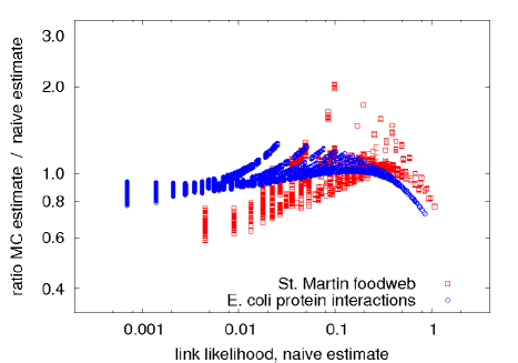
Figure 1: Log-log scatter plot of the naive analytic estimate of link likelihood $k_{out,i}k_{in,j}/L$ (directed network, St. Martin foodweb stmartin ) or $k_{i}k_{j}/2L$ (undirected network, Eschericia coli protein interaction network ecoli ) versus the ratio of the Monte-Carlo rewiring estimate to the naive estimate for the corresponding nodes. Note that the directed network has considerably more scatter for given $k_{out,i},k_{in,j}$.

For any ensemble $A$, let $N_{A}(k,k^{\prime})$ be the average number of links between nodes with degree $k$ and nodes with degree $k^{\prime}$. In terms of the link likelihood,

$$N_{A}(k,k^{\prime})=\sum_{i,j}p_{ij,A}\delta(k_{i}-k)\delta(k_{j}-k^{\prime})\quad$$ (6)

where the sum over $i,j$ indicates a sum over all pairs of nodes, and $p_{ij,A}$ is the link likelihood for ensemble $A$. If the ensemble $A$ is the trivial ensemble consisting of just one network, namely the experimentally observed graph ${\cal G}$ with adjacency matrix ${\cal M}_{\cal G}$, then $p_{ij,A}=M_{{\cal G},ij}$.

The average degree $\langle k^{\prime}\rangle_{k}$ of neighbors of nodes with degree $k$ is

$$\langle k^{\prime}\rangle_{k}=\frac{\sum_{k^{\prime}}k^{\prime}N(k,k^{\prime})}{\sum_{k^{\prime}}N(k,k^{\prime})}.$$ (7)

where we have dropped the subscript “$A$” for brevity. This quantity can be related to the (dis)assortativity, i.e. the tendency of nodes to connect (less) preferentially to nodes with similar degree. The assortativity was formally introduced by Newman as the Pearson correlation coefficient for the degrees of any two nodes connected by an edge newman02 . Intuitively, when the average degree $\langle k^{\prime}\rangle_{k}$ is an increasing function of $k$ then the network shows assortative mixing, i.e. nodes of low degree tend to connect to nodes of low degree and nodes of high degree tend to connect to nodes of high degree. When $\langle k^{\prime}\rangle_{k}$ is flat, the network shows no assortativity, and when $\langle k^{\prime}\rangle_{k}$ is a decreasing function of $k$ then the network shows disassortative mixing catanzaro .

We can compute $\langle k^{\prime}\rangle_{k}$ in several PFDS ensembles. The ensemble $Z_{3}(k_{1},k_{2})$ consists of uncorrelated random graphs with $N$ nodes, $L$ edges and no multiple or self-connections, where we fix the degrees of one pair of nodes. Evidently, we choose the pair whose link likelihood is being evaluated. Eq. (7) is then calculated by averaging over all pairs of nodes in the network. This clearly allows us to take the whole degree sequence into consideration, although only pairs of node degrees are considered simultaneously. To include the presence of a hub, we work in $Z_{4}(k_{1},k_{2},k_{\rm max})$, the ensemble of uncorrelated random graphs with $N$ nodes, $L$ edges and no multiple or self-connections, where we fix the degree of the pair of nodes whose link likelihood is being evaluated, as well as the degree $k_{\rm max}$ of the strongest hub.

As shown in Section V and in Appendix B, we can compute $\langle k^{\prime}\rangle_{k}$ exactly in $Z_{3}(k_{1},k_{2})$ and $Z_{4}(k_{1},k_{2},k_{\rm max})$, as well as in the approximate $Z_{3}(k_{1},k_{2})$ ensemble with $p_{ij}$ given by Eq.(1) [see also Eq. (22) below], which becomes exact in the limit of large $N$ for sparse networks, and for $k_{\rm max}\ll L$. In Fig. 2 we plot $\langle k^{\prime}\rangle_{k}$ versus $k$ for an Escherichia coli protein interaction network ecoli . The FDS ensemble, as sampled by the Monte Carlo rewiring procedure, is clearly disassortative, while the estimate of $\langle k^{\prime}\rangle_{k}$ using the standard naive estimate $p_{ij}=k_{i}k_{j}/2L$ shows no disassortativity or assortativity, as expected. We note that forbidding self-connection but otherwise using the naive estimate for $p_{ij}$ results in slight disassortativity, while approximate $Z_{3}$, exact $Z_{3}(k_{1},k_{2})$, and $Z_{4}(k_{1},k_{2},k_{\rm max})$ are increasingly refined estimates of the FDS behavior (see Fig. 2). Finally, $Z_{4}(k_{1},k_{2},k_{\rm max})$ gives only a slight improvement over $Z_{3}$, indicating that hubs per se are less important to global properties such as disassortativity than constraints such as no self- or multiple connections, which are already implemented at the level of $Z_{3}$, along with information about the whole degree sequence, taken in degree pairs.

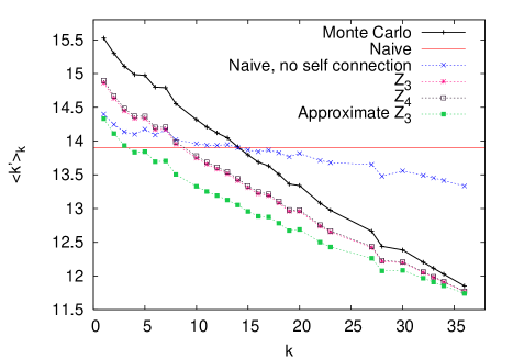
Figure 2: Average degree of the neighbor, $\langle k^{\prime}\rangle_{k}$ vs. node degree $k$ for an Escherichia coli protein interaction network  ecoli in several ensembles. The FDS ensemble, sampled by Monte Carlo rewiring, shows disassortativity as $\langle k^{\prime}\rangle_{k}$ is a decreasing function of $k$. For the naive estimate $p_{ij}=k_{i}k_{j}/2L$ and using the exact degree sequence, there is no disassortativity (while using a power law as in Eq. (10) leads to divergence). However, using the naive estimate but forbidding self-connection results in slight disassortativity. Approximate $Z_{3}$, exact $Z_{3}$, and $Z_{4}(k_{1},k_{2},k_{\rm max})$ are increasingly refined estimates of the FDS ensemble. Notice that the latter two can hardly be distinguished.

The approximate $Z_{3}$ ensemble is of further interest because $\langle k^{\prime}\rangle_{k}$ can be calculated analytically. Note that

$$N(k,k^{\prime}) = \sum_{i,j}p_{ij}^{model}\delta(k_{i}-k)\delta(k_{j}-k^{\prime})$$ (8)

$$= P(k,k^{\prime})N(k)N(k^{\prime}).$$

For a power law degree distribution,

$$N(k)=(\gamma-1)Nk^{-\gamma}$$ (9)

where $N$ is the number of nodes in the network and the degree distribution of the network is a power law with exponent $\gamma$. In this case the sums over $k^{\prime}$ in Eq. (7) can be approximated by integrals, yielding

$$\langle k^{\prime}\rangle_{k}=\frac{\int_{1}^{\infty}k^{\prime}P(k,k^{\prime})k^{\prime-\gamma}\;dk^{\prime}}{\int_{1}^{\infty}P(k,k^{\prime})k^{\prime-\gamma}\;dk^{\prime}}\;.$$ (10)

If we approximate $P(k,k^{\prime})$ by Eq. (1), these integrals can be solved in terms of hypergeometric functions:

$$\langle k^{\prime}\rangle_{k}=\frac{\gamma-1}{\gamma-2}\frac{{}_{2}F_{1}(1,\gamma-2;\gamma-1;\frac{-2L}{k})}{{}_{2}F_{1}(1,\gamma-1;\gamma;\frac{-2L}{k})}\;.$$ (11)

We note that for $\gamma=2.5$ the hypergeometric functions can be expressed in terms of elementary functions:

$$\langle k^{\prime}\rangle_{k}=\frac{\arcsin\left(\sqrt{\frac{2L}{2L+k}}\right)}{(\frac{k}{2L})^{1/2}-(\frac{k}{2L})\arctan\left((\frac{k}{2L})^{-1/2}\right)}.$$ (12)

To test the validity of Eq. (11), we turn to a large network, specifically Newman’s recent AS-level Internet data newmanInternet , for which $L=48436$. In park03 it is reported that $\gamma\approx 2.2\pm 0.3$ for the Internet; we estimate $\gamma\approx 2.1\pm 0.3$ for Ref. newmanInternet .

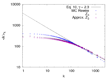
Figure 3: $\langle k^{\prime}\rangle_{k}$ versus $k$ for the Internet at the AS level from newmanInternet . We plot the analytic estimate of Eq. (11) for $\gamma=2.3$; for comparison we plot the results in the approximate $Z_{3}$ and $Z_{3}$ ensembles, computed directly from the degree sequence of newmanInternet , as well as Monte Carlo rewiring estimates of the FDS ensemble.

In Fig. 3 we plot the analytic estimates of $\langle k^{\prime}\rangle_{k}$ given by Eq. (11) for $\gamma=2.3$. This value for $\gamma$ gives the best fit for $\langle k^{\prime}\rangle_{k}$ and is within the uncertainty of the direct degree distribution measurement of $\gamma$. For comparison we also show the results in the approximate $Z_{3}$ and $Z_{3}$ ensembles, computed directly from the degree sequence of newmanInternet , as well as Monte Carlo rewiring estimates of the FDS ensemble. Note the strong similarities between the $Z_{3}$ results and the Monte Carlo estimates of the FDS ensemble; in particular, we observe a flattening of $\langle k^{\prime}\rangle_{k}$ for small $k$ both in the $Z_{3}$ ensemble and in the Monte Carlo rewiring. This is consistent with the observations of park03 .

Also note the similar scaling of the various estimates and of the Monte Carlo results at large $k$. For the Internet, $\langle k^{\prime}\rangle_{k}$ has been reported to scale with $k$ as a power law, $\langle k^{\prime}\rangle_{k}\approx k^{-\nu}$ with $\nu\approx 0.5$ park03 . Our Monte Carlo results for the FDS ensemble, using the degree sequence of Ref. newmanInternet , show indeed such a power law for large $k$, but with $\nu\approx 0.75$. The exact and approximate $Z_{3}$ calculations, obtained with the exact degree sequence, give $\nu\approx 0.7$ resp. $0.62$. When using a power law degree sequence and Eq. (11), the scaling depends on $\gamma$. But in this case, one can verify that scaling does not hold in the large $k$ limit, but in the limit $k\ll L$. The curvature of the continuous line visible in Fig. 3 results entirely from the fact that $k$ is not much less than $L$. Thus it is the slope of the continuous line at small $k$ which should be used for extracting $\nu$. With this, one finds that $\nu$ varies from $\approx 0.79$ for $\gamma=2.2$ to 0.5 for $\gamma=2.5$. Note that $\nu=0.5$ for $\gamma=2.5$ is an exact result that can be obtained analytically by taking the limit $2L/k/to\infty$ in Eq. (12).

In contrast to the approach of park03 , all of our results can be computed directly from the degree distribution or the degree sequence, omitting the intermediate step of constructing a fugacity distribution to match the statistics of the degree distribution and then extracting $\langle k^{\prime}\rangle_{k}$ from the fugacities. The fact that the disassortativity properties of the Internet can be studied so directly in the simple approximate $Z_{3}$ ensemble suggests that Eq. (1) should replace the naive estimate $P(k,k^{\prime})=kk^{\prime}/2L$ in other applications, for example in the study of motifs. This is explored in Section V.B (see Eq. 25).

For undirected networks and any null model $A$, Maslov et al. maslov04 defined a quantity called the correlation profile $R(k,k^{\prime})=N_{\cal G}(k,k^{\prime})/N_{A}(k,k^{\prime})$ and the ${\cal Z}$-score ${\cal Z}(k,k^{\prime})=[N_{\cal G}(k,k^{\prime})-N_{A}(k,k^{\prime})]/\sigma_{A}(k,k^{\prime})$, where $N_{A}(k,k^{\prime})$ is defined as in Eq. (6), $N_{\cal G}(k,k^{\prime})$ is the analogous quantity for the trivial ensemble (with $p_{ij}$ replaced by $M_{{\cal G},ij}$), and $\sigma^{2}_{A}(k,k^{\prime})$ is the variance of the number of links connecting nodes with degrees $k$ and $k^{\prime}$ in ensemble $A$ (remember that $N_{A}(k,k^{\prime})$ was the average of that number). The specific null studied in maslov04 was the FDS ensemble. As shown in Appendix A, a similar analysis can be done comparing different null models to each other. Results are also discussed in Appendix A.

V Analytic Estimates of the FDS ensemble for Undirected Networks

V.1 Notation and Basic Identities

We now derive our principal analytic results. Our central object is the partition function $Z$, which counts the number of graphs in the ensemble. The elementary constraints on the network ($N$ nodes, no multiple or self-connections) imply that the adjacency matrix $\cal M$ is $N\times N$, is symmetric (for undirected networks), has zeroes along the diagonal, and consists solely of $0$’s and $1$’s. If we add the constraint of $L$ links, the partition function can be written as

$$Z_{1}(N,L)=\sum_{\stackrel{{\scriptstyle\{M_{ij}=0,1\}}}{{i<j}}}\delta(L-\sum_{i<j}M_{ij})$$ (13)

where the sum is over the upper triangle of $\cal M$ due to symmetry. A simple computation gives Eq.(3) for the number of ways to distribute $L$ links among ${N\choose 2}$ possible pairs of nodes.

Now let us specify the degrees of $m$ of the nodes. We refer to $m$ as the “order” of a calculation. The partition function becomes

$$Z_{m+1}(N,L,k_{1},...,k_{m})=\sum_{\stackrel{{\scriptstyle\{M_{ij}\}}}{{i<j}}}\delta(L-\sum_{i<j}M_{ij})\\ \times\prod_{l=1}^{m}\delta(k_{l}-\sum_{j=1}^{l-1}M_{jl}-\sum_{j=l+1}^{N}M_{lj})$$ (14)

where we use the symmetry of the adjacency matrix to write the degree constraints in terms of the variables $M_{ij}$ with $i<j$.

It will be helpful at this point to introduce some further notation to assist us in organizing this calculation. We split the matrix $\cal M$ into four pieces:

• ${\cal A}$, the square submatrix controlling the edges linking the $m$ nodes with fixed degree to each other;

• ${\cal B}$, the rectangular matrix encoding the connections of the $m$ nodes of fixed degree with the rest of the nodes in the graph, and its transpose ${\cal B}^{T}$;

• ${\cal C}$, the square submatrix encoding the edges among the $N-m$ remaining nodes (whose degrees are not specified).

Due to the symmetry of $\cal M$ only $\cal B$ and the upper triangular parts of ${\cal A}$ and ${\cal C}$ are independent. In Fig. 4 we present a schematic decomposition of $\cal M$.

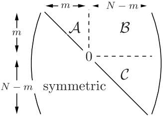
Figure 4: Schematic decomposition of the adjacency matrix $\cal M$ into the three sub-matrices ${\cal A,B,C}$ discussed in the text. Note that $\cal M$ is symmetric for undirected networks.

The sum over all adjacency matrices decomposes into a sum over the ${\cal A}$, $\cal B$ and $\cal C$ sub-matrices, with suitable constraints. In particular, we write the symbol $\sum_{\{\cal A\}}$ for the sum over all possible values $\{0,1\}$ of the matrix elements of the submatrix ${\cal A}$. Each term of this sum corresponds to a particular (possibly disconnected) labelled subgraph involving $m$ nodes of fixed degree. This is analogous to a diagrammatic expansion of the partition function, where the partition function is now written as the sum over all possible subgraphs involving nodes $1$ through $m$, and each subgraph is weighted by a degeneracy factor resulting from the summations over $\cal B$ and $\cal C$. This degeneracy counts the number of possible graphs in the ensemble containing that particular subgraph (respectively submatrix) ${\cal A}$. The partition function is written in this notation as:

$$Z_{m+1}=\sum_{\{\cal A\}}Z_{m+1}({\cal A})$$ (15)

where $Z_{m+1}({\cal A})$ is the partition function or degeneracy factor for a given fixed submatrix (equivalently, subgraph) $\cal A$. For each $Z_{m+1}({\cal A})$, the nodes with fixed degrees (i.e. the first $m$ nodes) are connected in a specified way. Thus, for example, the probability of some particular $m\times m$ subgraph $\cal A$ occurring would be

$${\rm Prob}({\cal A})=\frac{Z_{m+1}({\cal A})}{Z_{m+1}}\;.$$ (16)

As shown in Appendix B, the degeneracy of a given subgraph $Z_{m+1}({\cal A})$ can be written as

$$Z_{m+1}({\cal A})={{N-m\choose 2}\choose{L+\sum_{i<j,=2}^{j=m}A_{ij}-\sum_{l=1}^{m}k_{l}}}\\ \times\prod_{l=1}^{m}{N-m\choose k_{l}-\sum_{j=1}^{l-1}A_{jl}-\sum_{j=l+1}^{m}A_{lj}}$$ (17)

The first term on the right hand side is the degeneracy associated with the upper half triangle of the square submatrix $\cal C$. Recall that the submatrix $\cal C$ defines connections between all $N-m$ nodes not in $\cal A$, i.e. all nodes with free degree. This matrix has ${N-m\choose 2}$ independent places to put a specified number of 1’s. The number of 1’s in $\cal C$ depends on $L$, the total number of 1’s in the entire (upper triangular) adjacency matrix, minus the number of 1’s from edges that have at least one end on a node of fixed degree. By definition, those 1’s cannot appear in $\cal C$. Due to the symmetry of the entire matrix, the number of 1’s to be placed in the upper triangular half of $\cal C$ is $L+\sum_{i<j,j=2}^{j=m}A_{ij}-\sum_{l=1}^{m}k_{l}$.

Each factor in the product $\prod_{l=1}^{m}$ of Eq. (17) is the degeneracy associated with a row in the matrix $\cal B$. For every such row there are $N-m$ places to put 1’s, and the number of 1’s that must be placed in the $l$-th row is the degree of the node $k_{l}$ minus the number of 1’s in the corresponding row of the entire matrix $\cal A$. This latter number is the degree of the node within the subgraph $\cal A$.

V.2 Calculation of link likelihoods for undirected networks

As a first application we compute the link likelihood for two nodes in this framework. At lowest order we can just specify the degrees of the two nodes under consideration, giving the ensemble $Z_{3}$ with $m=2$. For convenience, the two nodes are labelled $1$ and $2$. The two possible configurations of this subsystem, where the nodes are either connected or disconnected, must be weighted by the appropriate degeneracy factors according to Eq. 17. Let us denote these two configurations by $\aleph$ and $\aleph^{\prime}$. In $\aleph$ an edge connects the two nodes, so $\aleph_{12}=1$. We denote this “connected” part of the total partition function $Z_{3}^{conn}=Z_{3}(\aleph)$. In $\aleph^{\prime}$ there is no edge between the two nodes, so $\aleph^{\prime}_{12}=0$. We denote this “disconnected” part of the total partition function $Z_{3}^{disc}=Z_{3}(\aleph^{\prime})$. The total partition function is thus $Z_{3}^{total}=Z_{3}^{conn}+Z_{3}^{disc}=Z_{3}(\aleph)+Z_{3}(\aleph^{\prime})$, thus

$$p^{(m=2)}_{12}=\frac{Z_{3}^{conn}}{Z_{3}^{total}}=\frac{Z_{3}(\aleph)}{Z_{3}(\aleph)+Z_{3}(\aleph^{\prime})}\;.$$ (18)

From Eq. 17, the explicit expressions are

$$Z_{3}(\aleph)={{N-2\choose 2}\choose L+1-k_{1}-k_{2}}\prod_{l=1}^{2}{N-2\choose k_{l}-1}\quad,$$ (19)

$$Z_{3}(\aleph^{\prime})={{N-2\choose 2}\choose L-k_{1}-k_{2}}\prod_{l=1}^{2}{N-2\choose k_{l}}\quad.$$ (20)

Straightforward calculation gives

$$p \!\!\!\!\!\!\!{}^{(m=2)}_{12}$$

$$\!\!\!\!\!\!=\left[1+\frac{(L+1-k_{1}-k_{2})(N-1-k_{1})(N-1-k_{2})}{k_{1}k_{2}((N-2)(N-3)/2-L+k_{1}+k_{2})}\right]^{-1}$$

and in the limit $L\to\infty$, $L/N^{2}\to 0$, and $k_{i}\ll L$ this reduces to

$$p^{(m=2)}_{12}\approx\frac{k_{1}k_{2}}{2L+k_{1}k_{2}}.$$ (22)

In the limit $k_{1}k_{2}<<L$ we recover from Eq. (22) the naive estimate $k_{1}k_{2}/2L$ used by most authors. This naive estimate is a bad approximation if either node 1 or node 2 is a hub. In general, the full expression given in Eq. (21) is a better approximation, although as we have shown in section IV the approximate $Z_{3}$ ensemble given by Eq. (22) is both analytically tractable and significantly better than the naive estimate.

The presence of any hubs in the network reduces the link likelihood between two nodes, particularly nodes of low degree, as their links are “stolen” by the hubs. This effect already appears in the calculation of the disassortativity, as shown in Figures 2 and 3. We can refine the preceding computation by including constraints on the degree sequence coming from the hubs. We incorporate these constraints from the hubs by considering the nodes with the highest degrees first. The partially fixed degree sequence ensemble $Z_{4}(k_{1},k_{2},k_{\rm max})$, then, includes the two nodes $k_{1},k_{2}$ whose link likelihood we compute (free to vary over all node pairs) and the largest hub in the network, with degree ($k_{\rm max}$). In the case that $k_{\rm max}=k_{1}$ or $k_{2}$ we use the next largest hub degree for the third constraint. In the sub-matrices $\cal A$, all possible ways to connect the three nodes are enumerated. To compute the link likelihood $p^{(m=3)}_{ij}$ we divide the partition function into connected $Z_{4}^{conn}$ and disconnected $Z_{4}^{disc}$ parts, where connected means an edge connects node 1 and node 2, i.e. $A_{12}=1$. The diagrammatic expansion for the connected sub-partition function is shown in Fig. 5a. and the disconnected sub-partition function is shown in Fig. 5b.

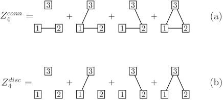
Figure 5: Diagrammatic expansion for the connected (a) and disconnected (b) contributions to the partition function $Z_{4}$ for $p_{12}$.

So we can compute the link likelihood as

$$p^{(m=3)}_{12} = \frac{Z_{4}^{conn}}{Z_{4}^{conn}+Z_{4}^{disc}}$$

$$= \frac{Z_{4}(\aleph_{1})+Z_{4}(\aleph_{2})+Z_{4}(\aleph_{3})+Z_{4}(\aleph_{4})}{\sum_{i=1}^{8}Z_{4}(\aleph_{i})}\quad,$$

where $\aleph_{1}$ to $\aleph_{8}$ denote the adjacency matrices for the eight graphs shown in Fig. 5. In Fig. 6 we compare the link likelihood $p_{ij}$ for an undirected network in the FDS ensemble (obtained numerically by the rewiring method) to the analytic results in the ensembles $Z_{3}(k_{1},k_{2})$ and $Z_{4}(k_{1},k_{2},k_{\rm max})$. For each pair $(i,j)$ we plot the naive estimate $\frac{k_{i}k_{j}}{2L}$ on the horizontal axis; the vertical coordinate is the ratio of the numerical (Monte-Carlo) estimate to the naive, no hub, and one hub estimates for that pair. The $Z_{3}$ estimate is already a substantial improvement over the naive analytic estimate, with slight further refinement coming as expected from the inclusion of hubs in all the diagrams.

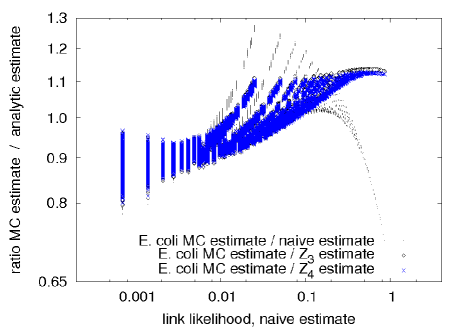
Figure 6: Scatter plot comparing estimates of the link likelihood in an Escherichia coli protein interaction network. On the horizontal logarithmic axis we plot the naive estimate $\frac{k_{i}k_{j}}{2L}$; on the vertical logarithmic axis we plot for all corresponding nodes the ratio of the Monte-Carlo rewiring estimate to the naive, $Z_{3}$ (no hub), and $Z_{4}$ (one hub) estimates. The latter two nearly coincide.

Table 1: Comparing estimates of the total number of triangles in various networks with $N$ nodes. MC refers to Monte Carlo rewiring estimates of the FDS ensemble. As expected, the results of Eq. 24 approach the asymptotic result, Eq. (25), for large, sparse networks.

Network	$N$	Eq. (25)	Eq. (24)	MC	% Error	% Error	% Error
					Eq. (25) vs. Eq. (24)	Eq. (25) vs. MC	Eq. (24) vs. MC
E. coli	230	215.82	289.65	322.14	25.49	33.01	10.09
Yeast(narrow)	1373	302.77	247.65	339.10	-22.26	10.71	26.97
Yeast	1373	651.07	592.59	1160.39	-9.87	43.89	48.93
Yeast (broad)	1373	1553.94	1667.70	2813.37	6.82	44.77	40.72
AS Internet	22963	29157.38	31840.23	37810.68	8.43	22.89	15.79
WWW	325729	379371.15	379706.63	274926.89	0.09	-37.99	-38.11

V.3 Calculation of subgraph likelihoods for undirected networks

Estimating the likelihoods of larger subgraphs can be done along exactly the same lines. As an example, we estimate the number of triangles in an undirected network and test this estimate on an Escherichia coli protein interaction network ecoli , a yeast (Saccharomyces cerevisiae) protein interaction network yeast , two artificial yeast protein interaction networks created by modifying the degree sequence of yeast by hand to make it narrower or broader, the Newman AS level map of the Internet newmanInternet , and a symmetrized snapshot of the World Wide Web WWW . Working in an ensemble with four constraints, $Z_{4}(k_{1},k_{2},k_{3})$, we consider all permitted triples of nodes $(i,j,k)$, forbidding self- and multiple connection. Note that node 3 is no longer fixed as the largest hub, but allowed to range over all nodes. Given fixed nodes 1, 2, and 3, we can compute the likelihood of a triangle between them as

$$p^{(m=3)}_{\Delta}=\frac{Z_{4}(\aleph_{4})}{\sum_{i=1}^{8}Z_{4}(\aleph_{i})}$$ (24)

where $\aleph_{4}$ corresponds to the fully connected subgraph, i.e. the last term in the sum of Fig. 5(a). The resulting combinatorial expression is quite unwieldy. However, in the limit $L\to\infty$, $L/N^{2}\to 0$, and $1\ll k_{i}\ll L$, i.e. the large, sparse network limit used in deriving Eq. (22) with the additional assumption of $1\ll k_{i}$, we find a remarkable simplification. The expression factorizes to

$$p^{(m=3)}_{\Delta}\approx P(k_{1},k_{2})P(k_{1},k_{3})P(k_{2},k_{3})$$ (25)

where $P(k_{1},k_{2})$ is given by Eq. (1).

We now test these formulae against the various trial networks. The results are shown in Table I, where “MC” represents the averaged triangle count for many Monte Carlo rewirings, i.e. a numerical estimate of the average number of triangles in the FDS ensemble. The only noticeable trend is the decrease in the absolute value of the % Error (defined as [Eq. (24) - Eq. (25)]/Eq. (24)) between the simple factorized expression of Eq. (25) and the elaborate expression of Eq. (24) as $N$ increases. This verifies the approximation made in deriving Eq. (25). The time required to make the “complex” estimate given by Eq. 24 is roughly equal to the time required to count the number of triangles for a single Monte Carlo instance; the simple estimate given by Eq. (25) is much faster, running on the WWW data in roughly $90$ seconds (on an Intel core duo processor) without any optimization for speed.

It is tedious to verify similar factorizations for larger motifs. However, the convergence to Eq. (25) in the predicted limit provides further evidence for the replacement of the naive estimate $P(k,k^{\prime})=kk^{\prime}/2L$ used e.g. in itzkovitz03 , where factorizations as in Eq. (25) were assumed, with Eq. (1). This will be the topic of future work. Such extensions of our method can also be used to study larger motifs in complex networks mayakim ; mayapeterkim , or to study large networks where computational time for rewiring grows prohibitively, but the approximation underlying Eqs. (22) and (25) should still be valid.

VI Conclusion

Detecting and describing local structure is an important frontier in the study of complex networks, as many of the features distinguishing real-world networks from their random analogues or null models are local: degree-degree correlations, motifs, and so forth. One of the major obstacles to this project is the lack of analytical techniques to study the fixed degree sequence ensemble, which is the most common null model for complex networks associated with the rewiring method. In this paper we have reviewed the numerical tools for studying the FDS ensemble and discussed some of the practical uses (e.g. disassortativity, motif calculation, correlation profiles) to which knowledge of local structure can be put. Through a careful study of the partition function of the FDS ensemble and the PFDS ensembles containing it, we derive simple and general combinatorial expressions that improve naive estimates of the link likelihood by explicitly including important constraints from the FDS ensemble (the exclusion of multiple edges and self connections, and the appearance of a broad range of degrees) in a “Gaussian” type approximation where the set of degree constraints are treated minimally but non-trivially.

In particular, for undirected networks we have developed the analytically tractable approximate $Z_{3}$ ensemble, where the link likelihood $P(k,k^{\prime})=kk^{\prime}/(2L+kk^{\prime})$ (Eq. (1)) gives clear disassortativity, while the naive estimate $kk^{\prime}/2L$ does not. We have also introduced a diagrammatic expansion of the PFDS partition function, which organizes the combinatorial calculations usefully and leads to a simple, approximate factorized formula for the estimated number of undirected triangles between three nodes, $P_{\Delta}^{(m=3)}(k_{1},k_{2},k_{3})=P(k_{1},k_{2})P(k_{1},k_{3})P(k_{2},k_{3})$ (Eq. (25)) where $k_{1},k_{2},k_{3}$ are the degrees of the $3$ nodes. The factorization suggests the application of Eq. (22) to extended local structures such as motifs.

It should be emphasized that these analytic results are not merely useful for the null model they have been explicitly developed to approximate (the FDS ensemble). They also provide guidance in developing more complicated null models that incorporate higher-level constraints. The astronomical $\cal{Z}$-scores observed in work on extended motifs mayakim ; mayapeterkim dramatize the need for such extensions, which might constrain, for example, the number of triangles in addition to the number of nodes, number of links, and a few degrees. Further work will explore applications of the approximate $Z_{3}$ and other PFDS ensembles to motif estimates, as well as the incorporation of higher-level constraints in the PFDS ensemble to improve likelihood estimates of extended motifs. The extension of the results of this paper to directed networks is in preparation.

VII Appendix A: Comparing null models via the correlation profile

We can study how the real network deviates from various null hypotheses by calculating $R(k,k^{\prime})$ with respect to various null hypotheses. This provides an overall measure of how close the ensembles are to each other and helps establish the relevant features that distinguish the real network from the different ensembles.

In general, we can define correlation profiles and ${\cal Z}$-scores for any pair $\left(A,B\right)$ of ensembles:

$$R_{A|B}(k,k^{\prime})=\frac{N_{A}(k,k^{\prime})}{N_{B}(k,k^{\prime})}.$$ (26)

and

$${\cal Z}_{A|B}(k,k^{\prime})=\frac{N_{A}(k,k^{\prime})-N_{B}(k,k^{\prime})}{\sqrt{\sigma_{A}^{2}+\sigma_{B}^{2}}}.$$ (27)

In particular, we can calculate the correlation profile for the numerically sampled FDS ensemble and the ensemble $Z_{3}(k_{1},k_{2})$. Recall that the ensemble $Z_{3}$ consists of uncorrelated random graphs with $N$ nodes, $L$ edges and no multiple or self- connections, where we fix the degree of the pair of nodes whose link likelihood is being evaluated. We might also compare the FDS ensemble to $Z_{4}(k_{1},k_{2},k_{\rm max})$, the ensemble of uncorrelated random graphs with $N$ nodes, $L$ edges and no multiple or self-connections, where we fix the degree of the pair of nodes whose link likelihood is being evaluated, as well as the degree of the largest node in the network, $k_{\rm max}$. In $Z_{3}$ and $Z_{4}$, $p_{ij}$ can be calculated exactly (see Section V). We plot $R_{Z_{3}|\rm{FDS}}(k,k^{\prime})$ for the Escherichia coli protein interaction network in Fig. 7. It is clear that the $Z_{3}$ ensemble captures many of the features of the FDS ensemble, as $R_{Z_{3}|\rm{FDS}}(k,k^{\prime})$ is close to $1$ for all $k,k^{\prime}$. $R_{Z_{4}|\rm{FDS}}(k,k^{\prime})$ exhibits slight improvement over $Z_{3}$, as expected (data not shown). The correlation profile allows us to identify correlations due to the degrees of the other nodes in the network and provides a test of our hypothesis that the PFDS ensemble captures much of the structure of the FDS ensemble.

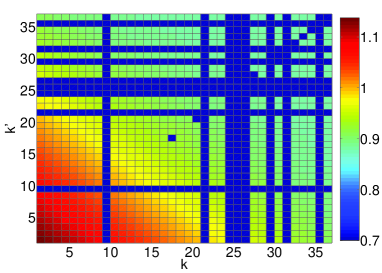
Figure 7: Correlation profile $R_{Z_{3}|\rm{FDS}}(k,k^{\prime})$ for the Escherichia coli protein interaction network ecoli . Note that the dark blue regions are artificially set to the value $.7$; they correspond to values of $(k,k^{\prime})$ for which no data exist.

VIII Appendix B: Derivation of $Z_{m+1}$ for Undirected networks

We note that the number of possible undirected subgraphs of $m$ nodes is $2^{(m^{2}-m)/2}$. So we write:

$$Z_{m+1}(N,L,k_{1},...,k_{m}) =$$

$$\sum_{\{A_{ij}\}}\sum_{\{B_{ij}\}}\sum_{\{C_{ij}\}}\delta(L-(\sum_{\stackrel{{\scriptstyle i<j}}{{j=2}}}^{j=m}A_{ij})-(\sum_{\stackrel{{\scriptstyle i\leq m}}{{j=m+1}}}^{j=N}B_{ij})-(\sum_{\stackrel{{\scriptstyle i<j}}{{i=m+1}}}^{i=N}C_{ij}))$$

$$\times\prod_{l=1}^{m}\delta(k_{l}-\sum_{j=1}^{l-1}A_{jl}-\sum_{j=l+1}^{m}A_{lj}-\sum_{j=m+1}^{N}B_{lj})$$ (28)

For concision we henceforth write the sum more compactly, as in the next equation.

We now Fourier transform the delta-functions:

$$Z_{m+1}(N,L,k_{1},...,k_{m}) =\sum_{\{\cal ABC\}}\frac{1}{(2\pi)^{m+1}}\int_{-\pi}^{\pi}...\int_{-\pi}^{\pi}dzda_{1}...da_{m}e^{\imath z(L-\sum_{\stackrel{{\scriptstyle i<j}}{{j=2}}}^{j=m}A_{ij})}$$

$$\times\prod_{l=1}^{m}e^{\imath a_{l}(k_{l}-\sum_{j=1}^{l-1}A_{jl}-\sum_{j=l+1}^{m}A_{lj})}\prod_{l=1}^{m}\prod_{j=m+1}^{N}e^{-\imath(z+a_{l})B_{lj}}\prod_{\stackrel{{\scriptstyle i<j}}{{i=m+1}}}^{N}e^{-\imath zC_{ij}}$$ (29)

We can do the sum over $B_{ij}$, yielding:

$$Z_{m+1}(N,L,k_{1},...,k_{m}) =\sum_{\{\cal AC\}}\frac{1}{(2\pi)^{m+1}}\int_{-\pi}^{\pi}...\int_{-\pi}^{\pi}dzda_{1}...da_{m}e^{\imath z(L-\sum_{\stackrel{{\scriptstyle i<j}}{{j=2}}}^{j=m}A_{ij})}$$

$$\times\prod_{l=1}^{m}e^{\imath a_{l}(k_{l}-\sum_{j=1}^{l-1}A_{jl}-\sum_{j=l+1}^{m}A_{lj})}\prod_{l=1}^{m}(1+e^{-\imath(z+a_{l})})^{N-m}\prod_{\stackrel{{\scriptstyle i<j}}{{i=m+1}}}^{N}e^{-\imath zC_{ij}}$$ (30)

Performing the standard binomial expansion yields:

$$Z_{m+1}(N,L,k_{1},...,k_{m}) =\sum_{\{\cal AC\}}\frac{1}{(2\pi)^{m+1}}\int_{-\pi}^{\pi}...\int_{-\pi}^{\pi}dzda_{1}...da_{m}e^{\imath z(L-\sum_{\stackrel{{\scriptstyle i<j}}{{j=2}}}^{j=m}A_{ij})}$$

$$\times\prod_{l=1}^{m}e^{\imath a_{l}(k_{l}-\sum_{j=1}^{l-1}A_{jl}-\sum_{j=l+1}^{m}A_{lj})}\prod_{l=1}^{m}\sum_{n_{l}=0}^{N-m}{N-m\choose n_{l}}e^{-\imath n_{l}(z+a_{l})}\prod_{\stackrel{{\scriptstyle i<j}}{{i=m+1}}}^{N}e^{-\imath zC_{ij}}$$ (31)

Integrating over $a_{1}...a_{m}$ sets $n_{l}=k_{l}-\sum_{j=1}^{l-1}A_{jl}-\sum_{j=l+1}^{m}A_{lj}$, so we have:

$$Z_{m+1}(N,L,k_{1},...,k_{m}) =\sum_{\{\cal AC\}}\frac{1}{(2\pi)}\int_{-\pi}^{\pi}dze^{\imath z(L-\sum_{\stackrel{{\scriptstyle i<j}}{{j=2}}}^{j=m}A_{ij})}$$

$$\times\prod_{l=1}^{m}e^{-\imath z(k_{l}-\sum_{j=1}^{l-1}A_{jl}-\sum_{j=l+1}^{m}A_{lj})}{N-m\choose k_{l}-\sum_{j=1}^{l-1}A_{jl}-\sum_{j=l+1}^{m}A_{lj}}\prod_{\stackrel{{\scriptstyle i<j}}{{i=m+1}}}^{N}e^{-\imath zC_{ij}}$$ (32)

We now sum over ${C_{ij}}$ and perform the binomial expansion of the resulting quantity:

$$Z_{m+1}(N,L,k_{1},...,k_{m}) =\sum_{\{\cal A\}}\frac{1}{(2\pi)}\int_{-\pi}^{\pi}dze^{\imath z(L+\sum_{\stackrel{{\scriptstyle i<j}}{{j=2}}}^{j=m}A_{ij}-\sum_{l=1}^{m}k_{l})}$$

$$\times\prod_{l=1}^{m}{N-m\choose k_{l}-\sum_{j=1}^{l-1}A_{jl}-\sum_{j=l+1}^{m}A_{lj}}\sum_{n=0}^{{N-m\choose 2}}{{N-m\choose 2}\choose n}e^{-\imath zn}$$ (33)

where we have used the fact that

$$\prod_{l=1}^{m}e^{\imath z(\sum_{j=1}^{l-1}A_{jl}+\sum_{j=l+1}^{m}A_{lj})}=e^{\imath z(\sum_{l=1}^{m}(\sum_{j=1}^{l-1}A_{jl}+\sum_{j=l+1}^{m}A_{lj}))}=e^{2\imath z\sum_{\stackrel{{\scriptstyle l<j}}{{j=2}}}^{j=m}A_{lj}}$$

by the symmetry of the adjacency matrix. We may now integrate over $z$ to give the result:

$$Z_{m+1}(N,L,k_{1},...,k_{m})=\sum_{\{{\cal A}\}}{{N-m\choose 2}\choose(L+\sum_{i<j,j=2}^{j=m}A_{ij}-\sum_{l=1}^{m}k_{l})}\prod_{l=1}^{m}{N-m\choose k_{l}-\sum_{j=1}^{l-1}A_{jl}-\sum_{j=l+1}^{m}A_{lj}}$$ (34)

This can be written as a sum over sub-partition sums $Z_{m+1}({\cal A})$, each of which is given by Eq. (17). Thus we recover the result for fixed $\cal A$ given in Section V.

References

- (1) J. Theiler, S. Eubank, A. Longtin, B. Galdrikian, and J.D. Farmer, Physica D 58, 77 (1992).
- (2) T. Schreiber and A. Schmitz, Physica D 142, 346 (2000).
- (3) S. Maslov and K. Sneppen, Science 296, 910 (2002).
- (4) R. Milo, N. Kashtan, S. Itzkovitz, M.E.J. Newman, U. Alon, preprint arXiv/cond-mat/0312028v2 (2004).
- (5) Y.G. Chen, P. Diaconis, S.R. Holmes, and J.S. Liu, J. Amer. Statist. Assoc. 100, 109 (2005).
- (6) M.E.J. Newman, SIAM Review 45, 167-256, preprint arXiv/cond-mat/0303516v1 (2003).
- (7) M.E.J. Newman, Phys. Rev. E 64, 016131 (2001).
- (8) S. Gupta, R.M. Anderson, and R.M. May, AIDS 3, 807-817 (1989).
- (9) M. Kretzschmar, Y.T.H.P. van Duynhoven, and A.J. Severijnen, Am. J. Epidemiol. 144, 306-317 (1996).
- (10) J. Camacho, R. Guimerà, and L.A.N. Amaral, Phys. Rev. Lett. 88, 228102 (2002).
- (11) S.A. Kauffman in A. Moscana and A. Monroy (eds.) Current Topics in Developmental Biology 6, 145-182 (Academic Press, New York, 1971).
- (12) J. Davidsen, P. Grassberger, M. Paczuski, Geophys. Res. Lett., 33, L11304 (2006).
- (13) M. Paczuski, “Networks as Renormalized Models for Emergent Behavior in Physical Systems”, in C. Beck, G. Benedek, A. Rapisarda & C. Tsallis (eds.) Complexity, Metastability and Nonextensivity (World Scientific, London, 2005).
- (14) R. Albert and A.-L. Barabási, Rev. Mod. Phys. 74, 47 (2002).
- (15) A.S.N. Dorogovtsev and J.F.F. Mendes, Adv. Phys. 51, 1079 (2002).
- (16) B. Bollobas, Random graphs (Cambridge Univ. Press, 2001).
- (17) This is the number of ways of placing identical objects (in this case “1”s) in places.
- (18) J. Park and M.E.J. Newman, Phys. Rev. E 68, 026112 (2003).
- (19) J. Park and M.E.J. Newman, Phys. Rev. E 70, 066117 (2004).
- (20) L. Bogacz, Z. Burda, and B. Waclaw, Physica A, 366, 587 (2006).
- (21) B.Y. Wang and F. Zhang, Discrete Math. 187, 211 (1998).
- (22) E.A. Bender and E.R. Canfield, Journal of Combinatorial Theory A 24, 296-307 (1978).
- (23) R. Milo, S. Shen-Orr, S. Itzkovitz, N. Kashtan, D. Chklovskii, and U. Alon, Science 298, 824 (2002).
- (24) S.J. Liu, Monte Carlo Strategies in Scientific Computing (Springer, New York 2001).
- (25) P. Grassberger, Computer Physics Communications 147, 64 (2002).
- (26) J. Besag and P. Clifford, Biometrica 76, 633 (1989).
- (27) A.R. Rao, R. Jana, and S. Bandyopadhya, Indian J. Statistics 58, 225 (1996).
- (28) J.M. Roberts Jr., Social Networks 22, 273 (2000).
- (29) G.W. Cobb and Y.-P. Chen, American Mathematical Monthly 110, 265 (2003).
- (30) In many cases one wants to construct a surrogate ensemble with the same degree sequence as a given graph . If a given graph is available, one does not need this first step, and starts from directly.
- (31) H.J. Ryser, Can. J. Math. 9, 371 (1957).
- (32) F.T. Wall and J.J. Erpenbeck, J. Chem. Phys. 30, 634 (1959).
- (33) S. Maslov, K. Sneppen, and A. Zaliznyak, Physica A 333, 529 (2004).
- (34) M.E.J. Newman, Phys. Rev. Lett. 89, 208701-1 (2002); Phys. Rev. E 67, 026126 (2003). Phys. Rev. E 68, 026127 (2003).
- (35) P. Mahadevan, D. Krioukov, K. Fall, and A. Vahdat, “A Basis for Systematic Analysis of Network Topologies”, SIGCOMM ’06, preprint arXiv/cs.NI/0605007v2 (2006).
- (36) M. Catanzaro, M. Boguñá, R. Pastor-Satorras, Phys. Rev. E 71, 027103, preprint arXiv/cond-mat/0408110v1 (2005).
- (37) L. Goldwasser and J. Roughgarden, Ecology 74, 1216-1233 (1993).
- (38) G. Butland et al., Nature 433, 531 (2005).
-
(39)
M. Newman, data at URL
www-personal.umich.edu/mejn/netdata/ (2006). - (40) A.C. Gavin et al., Nature 440, 631 (2006); data received from G. Musso (University of Toronto).
- (41) R. Albert, H. Jeong and A.-L. Barabási, Nature 401, 130 (1999); data at www.nd.edu/networks/resources.htm.
- (42) S. Itzkovitz, R. Milo, N. Kashtan, G. Ziv, and U. Alon, Phys. Rev. E 68, 026127, preprint arXiv cond-mat/0302375 (2003).
- (43) K. Baskerville and M. Paczuski, Phys. Rev. E 74, 051903, preprint arXiv q-bio.QM/0606023 (2006).
- (44) K. Baskerville, P. Grassberger, and M. Paczuski, preprint arXiv q-bio/0702029 (2007).