One-Particle Anomalous Excitations of Gutzwiller-Projected BCS Superconductors and Bogoliubov Quasi-Particle Characteristics

Abstract

Low-lying one-particle anomalous excitations are studied for Gutzwiller-projected strongly correlated BCS states. It is found that the one-particle anomalous excitations are highly coherent, and the numerically calculated spectrum can be reproduced quantitatively by a renormalized BCS theory, thus strongly indicating that the nature of low-lying excitations described by the projected BCS states is essentially understood within a renormalized Bogoliubov quasi-particle picture. This finding resembles the well-known fact that a Gutzwiller-projected Fermi gas is a Fermi liquid. The present results are consistent with numerically exact calculations of the two-dimensional $t$-$J$ model as well as recent photoemission experiments on high-$T_{\rm C}$ cuprate superconductors.

Since their discovery in 1986 bed , high-$T_{\rm C}$ cuprate superconductors and related strongly correlated electronic systems have become one of the largest and most important fields in current condensed matter physics rvb . In spite of enormous theoretical and experimental efforts devoted since their discovery, understanding the mechanism of the superconductivity and the unusual normal state properties of the high-$T_{\rm C}$ cuprate superconductors remains unresolved and there is still extensive debate. This is mainly because of the strong-correlation nature of the problems, which is widely believed to be a key ingredient. Immediately after the discovery, Anderson pwa proposed a Gutzwiller-projected BCS state to incorporate strong-correlation effects in the superconducting state. While the ground state properties of projected BCS states have been studied extensively yokoyama , it is only very recently that the low-energy excitations of projected BCS states have been explored by numerically exact variational Monte Carlo techniques rand ; yunoki ; fukushima ; li , which in fact have found many qualitative as well as very often quantitative similarities to the main features observed experimentally in high-$T_{\rm C}$ cuprate superconductors. It is therefore very important and timely to understand the nature of low-lying excitations described by Gutzwiller-projected BCS states because of their great relevance to the high-$T_{\rm C}$ cuprate superconductors. Furthermore, a Gutzwiller projected single-particle state is one of the most widely used correlated many-body wave functions in a variety of research fields march ; org ; optical , and thus better understanding of the nature of projected BCS states is also highly desirable. This is precisely the main purpose of this study.

In this paper, one-particle anomalous excitations are studied for Gutzwiller-projected BCS superconductors. It is shown that one of the characteristic properties for the Gutzwiller-projected BCS states is their highly coherent one-particle anomalous excitations. It is found that the numerically calculated one-particle anomalous excitations can be reproduced quantitatively by a renormalized BCS theory. This finding thus strongly indicates that the low-lying excitations of the Gutzwiller-projected BCS states are described within a renormalized Bogoliubov quasi-particle picture, which resembles the well known fact that a Gutzwiller-projected Fermi gas is a Fermi liquid voll . The present results also provide a theoretical justification for utilizing a simple mean-field based BCS theory to analyze low-energy experimental observations for the high-$T_{\rm C}$ cuprate superconductors.

A Gutzwiller-projected BCS state $|\Psi_{0}^{(N)}\rangle$ with $N$ electrons is defined by

$$|{\Psi}_{0}^{(N)}\rangle={\hat{\cal P}}_{N}{\hat{\cal P}}_{G}|{\rm BCS}\rangle,$$ (1)

where $|{\rm BCS}\rangle=\prod_{{\bf k},\sigma}{\hat{\gamma}}_{{\bf k}\sigma}|0\rangle$ is the ground state of the BCS mean-field Hamiltonian text with singlet pairing and ${\hat{\gamma}}_{{\bf k}\sigma}$ is the standard Bogoliubov quasi-particle annihilation operator with momentum ${\bf k}$ and spin $\sigma(=\uparrow,\downarrow)$,

$$\left(\begin{array}[]{c}{\hat{\gamma}}_{{\bf k}\uparrow}\\ {\hat{\gamma}}^{\dagger}_{-{\bf k}\downarrow}\end{array}\right)=\left(\begin{array}[]{cc}u_{\bf k}^{*}&-v_{\bf k}^{*}\\ v_{\bf k}&u_{\bf k}\end{array}\right)\left(\begin{array}[]{c}{\hat{c}}_{{\bf k}\uparrow}\\ {\hat{c}}^{\dagger}_{-{\bf k}\downarrow}\end{array}\right),$$ (2)

${\hat{\cal P}}_{G}=\prod_{\bf i}(1-{\hat{n}}_{{\bf i}\uparrow}{\hat{n}}_{{\bf i}\downarrow})$ is the Gutzwiller projection operator excluding sites doubly occupied by electrons, and ${\hat{\cal P}}_{N}$ the projection operator onto even number $N$ of electrons. ${\hat{c}}_{{\bf k}\sigma}=\sum_{\bf i}{\rm e}^{-i{\bf k}\cdot{\bf i}}{\hat{c}}_{{\bf i}\sigma}/{\sqrt{L}}$ ($L$: number of sites) is the Fourier transform of the electron annihilation operator ${\hat{c}}_{{\bf i}\sigma}$ at site ${\bf i}$ with spin $\sigma$, and ${\hat{n}}_{{\bf i}\sigma}={\hat{c}}_{{\bf i}\sigma}^{\dagger}{\hat{c}}_{{\bf i}\sigma}$. Note that, since the number $N$ of electrons is even, $|\Psi^{(N)}_{0}\rangle$ is a spin singlet with zero total momentum. In the following, it is implicitly assumed that the gap function in $|{\rm BCS}\rangle$ is real and the spatial dimensionality is two dimensional (2D). However, the generalization of the present study is straightforward.

A single-hole (single-electron) added excited state $|\Psi^{(N-1)}_{{\bf k}\sigma}\rangle$ ($|\Psi^{(N+1)}_{{\bf k}\sigma}\rangle$) is similarly defined zhang ; rand ; ong ; yunoki ; yunoki2 by

$$|\Psi^{(N\pm 1)}_{{\bf k}\sigma}\rangle={\hat{\cal P}}_{N\pm 1}{\hat{\cal P}}_{G}{\hat{\gamma}}_{{\bf k}\sigma}^{\dagger}|{\rm BCS}\rangle,$$ (3)

which has momentum ${\bf k}$, total spin $1/2$, and $z$-component of total spin $\sigma$. Hereafter, the normalized wave functions for the $N$- and $(N\pm 1)$-particle states are denoted simply by $|\psi^{(N)}_{0}\rangle$ and $|\psi^{(N\pm 1)}_{{\bf k}\sigma}\rangle$, respectively. The quasi-particle weights for the one-particle added and removed normal excitations are thus defined as

$$Z_{+}^{(N)}({\bf k}\sigma)=\left|\langle\psi^{(N+1)}_{{\bf k}\sigma}|{\hat{c}}^{\dagger}_{{\bf k}\sigma}|\psi^{(N)}_{0}\rangle\right|^{2}$$ (4)

and

$$Z_{-}^{(N)}({\bf k}\sigma)=\left|\langle\psi^{(N-1)}_{-{\bf k}{\bar{\sigma}}}|{\hat{c}}_{{\bf k}\sigma}|\psi^{(N)}_{0}\rangle\right|^{2},$$ (5)

respectively, where ${\bar{\sigma}}$ is the opposite spin to $\sigma$.

The one-particle anomalous excitation spectrum is generally defined as

$$F({\bf k},\omega)=$$

$$-{\frac{1}{\pi}}{\rm Im}\left\langle\Phi_{0}^{(N+2)}\left|{\hat{c}}^{\dagger}_{{\bf k}\uparrow}{\frac{1}{\omega-{\hat{H}}+{\cal E}_{0}^{(N)}+i0^{+}}}{\hat{c}}^{\dagger}_{-{\bf k}\downarrow}\right|\Phi_{0}^{(N)}\right\rangle,$$

where $|\Phi_{n}^{(N)}\rangle$ is the $n$th eigenstate ($n=0,1,2,\cdots$, with 0 corresponding to the ground state) of a system described by Hamiltonian ${\hat{H}}$ with its eigenvalue ${\cal E}_{n}^{(N)}$ and $N$ electrons ohta . The spectral representation thus leads

$$F({\bf k},\omega)=\sum_{n=0}\left\langle\Phi_{0}^{(N+2)}\left|{\hat{c}}^{\dagger}_{{\bf k}\uparrow}\right|\Phi_{n}^{(N+1)}\right\rangle\quad\quad$$

$$\ \times\left\langle\Phi_{n}^{(N+1)}\left|{\hat{c}}^{\dagger}_{-{\bf k}\downarrow}\right|\Phi_{0}^{(N)}\right\rangle\delta\left(\omega-{\cal E}_{n}^{(N+1)}+{\cal E}_{0}^{(N)}\right).$$ (6)

Note that $F({\bf k},\omega)$ is a real function provided that spin rotation and reflection invariance as well as time reversal symmetry are assumed fermi . The frequency integral of the one-particle anomalous excitation spectrum, $F_{\bf k}^{(N)}=\int_{-\infty}^{\infty}d\omega F({\bf k},\omega)=\left\langle\Phi_{0}^{(N+2)}\left|{\hat{c}}^{\dagger}_{{\bf k}\uparrow}{\hat{c}}^{\dagger}_{-{\bf k}\downarrow}\right|\Phi_{0}^{(N)}\right\rangle$, provides a well-known sum rule which will be used later.

To study the one-particle anomalous excitations for the projected BCS state, let us first defined the following quantity similar to $F_{\bf k}^{(N)}$ for the projected BCS states:

$$Z_{2}^{(N)}({\bf k})=\left\langle\psi_{0}^{(N+2)}\left|{\hat{c}}^{\dagger}_{{\bf k}\uparrow}{\hat{c}}^{\dagger}_{-{\bf k}\downarrow}\right|\psi_{0}^{(N)}\right\rangle.$$ (7)

Here $|\psi_{0}^{(N+2)}\rangle$ is constructed in exactly the same way as $|\psi_{0}^{(N)}\rangle$ except that the number of electrons onto which the state is projected is $N+2$. Using the previously derived relations for the projected BCS states yunoki2 , one can now easily show that

$$Z_{2}^{(N)}({\bf k})=\left\langle\psi_{0}^{(N+2)}\left|{\hat{c}}^{\dagger}_{{\bf k}\uparrow}\right|\psi_{-{\bf k}\downarrow}^{(N+1)}\right\rangle\left\langle\psi_{-{\bf k}\downarrow}^{(N+1)}\left|{\hat{c}}^{\dagger}_{-{\bf k}\downarrow}\right|\psi_{0}^{(N)}\right\rangle,$$ (8)

i.e., as will be shown later, the quasi-particle weight for the one-particle anomalous excitations is $Z_{2}^{(N)}({\bf k})$. It is also interesting to notice that the above equation relates $Z_{2}^{(N)}({\bf k})$ to the quasi-particle weights for the one-particle normal excitations, i.e.,

$$\left|Z_{2}^{(N)}({\bf k})\right|^{2} = Z_{+}^{(N)}(-{\bf k}\downarrow)\cdot Z_{-}^{(N+2)}({\bf k}\uparrow),$$ (9)

which should be useful for computing $Z_{-}^{(N)}({\bf k}\sigma)$ note .

The validity of Eq. (9) can be checked numerically by computing all quantities, $Z_{+}^{(N)}(-{\bf k}\downarrow)$, $Z_{-}^{(N+2)}({\bf k}\uparrow)$, and $\left|Z_{2}^{(N)}({\bf k})\right|^{2}$, independently. A typical set of results calculated by a standard variational Monte Carlo technique on finite clusters is shown in Figs 1 (a) and (b), where one can see that indeed Eq. (9) holds within the statistical error note2 .

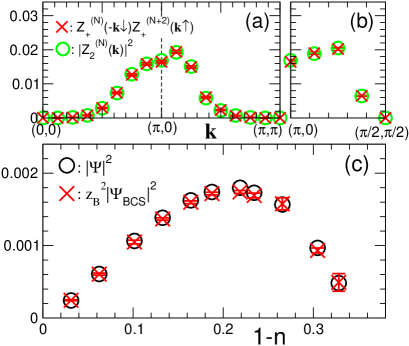
Figure 1: (Color online) (a) and (b): $\left|Z_{2}^{(N)}({\bf k})\right|^{2}$ (circles) and $Z_{+}^{(N)}(-{\bf k}\downarrow)\cdot Z_{-}^{(N+2)}({\bf k}\uparrow)$ (crosses) for different momenta ${\bf k}$ and $N=222$ $(n\approx 0.87)$. (c): $|\Psi|^{2}=|\langle\psi_{0}^{(N+2)}|c_{{\bf i}\uparrow}^{\dagger}c_{{\bf i}+{\bf x}\downarrow}^{\dagger}|\psi_{0}^{(N)}\rangle|^{2}$ (circles) as a function of electron density $n$. $|\psi_{0}^{(N)}\rangle$ is optimized for the 2D $t$-$t^{\prime}$-$J$ model with $t^{\prime}/t=-0.2$ and $J/t=0.3$ on an $L=16\times 16$ cluster with periodic boundary conditions yunoki ; note3 . For comparison, $z_{B}^{2}|\Psi_{\rm BCS}|^{2}$ for a renormalized BCS theory (see the text) is also presented by crosses in (c).

Now let us assume that there exists a system (with Hamiltonian ${\hat{H}}$) for which the ground state and the low-energy excited states can be described approximately by the projected BCS states $|\Psi_{0}^{(N)}\rangle$ and $|\Psi^{(N\pm 1)}_{\bf k}\rangle$, i.e., $|\Phi_{0}^{(N)}\rangle\approx|\Psi_{0}^{(N)}\rangle$ and $|\Phi_{n}^{(N+1)}\rangle\approx|\Psi^{(N+1)}_{\bf k}\rangle$, etc. One immediate consequence of this assumption is that the sum rule for $F({\bf k},\omega)$ is now $\int_{-\infty}^{\infty}d\omega F({\bf k},\omega)=Z_{2}^{(N)}({\bf k})$. Another consequence is that the spectral representation of the one-particle anomalous excitations is

$$F({\bf k},\omega) = Z_{2}^{(N)}({\bf k})\cdot\delta\left(\omega-E_{-{\bf k}}^{(N+1)}+E_{0}^{(N)}\right)$$ (10)

$$+ \sum_{n(\neq 0)}\,({\rm other\ terms}),$$

i.e., the quasi-particle weight for the one-particle anomalous excitations is $Z_{2}^{(N)}({\bf k})$. Here $E_{0}^{(N)}=E({\Psi}_{0}^{(N)})=\langle{\psi}_{0}^{(N)}|{\hat{H}}|{\psi}_{0}^{(N)}\rangle$, and $E_{-{\bf k}}^{(N+1)}=E({\Psi}_{-{\bf k}\downarrow}^{(N+1)})$. This is because of the equality derived here in Eq. (8). Since the spectral weight is not positive definite, the above equation along with the sum rule does not immediately imply that the contribution of incoherent “other terms” in Eq. (10) is negligible. However, using the property of the projected BCS states reported previously that the one-particle added normal excitations are coherent ong ; mohit ; yunoki2 , one can easily show that indeed the one-particle anomalous excitations consist of a single coherent part for each ${\bf k}$ with no incoherent contributions. It is interesting to note that numerically exact diagonalization studies of small clusters have also found that the one-particle anomalous excitations for the 2D $t$-$J$ model are highly coherent with relatively small incoherent contributions ohta .

Let us now calculate the one-particle anomalous excitation spectrum $F({\bf k},\omega)$ for the projected BCS states. For this purpose, here we will consider the 2D $t$-$t^{\prime}$-$J$ model on the square lattice yunoki . This model has been studied extensively and found to show a $d$-wave superconducting regime in the phase diagram tj ; ohta . Furthermore, it is well-known that a Gutzwiller-projected BCS state with $d$-wave pairing symmetry [Eq. (1)] is a faithful variational ansatz for the superconducting state of this model yokoyama . The model parameters used here are set to be $t^{\prime}/t=-0.2$ and $J/t=0.3$ elbio .

The results of the numerically calculated $F({\bf k},\omega)$ for representative momenta are shown in Fig. 2, where $|\Psi_{0}^{(N)}\rangle$ is optimized to minimize the variational energy for $N=222$ on an $L=16\times 16$ cluster $(n\approx 0.87)$ with periodic boundary conditions note3 . As is expected for a $d$-wave superconductor, the spectral weight becomes smaller toward the nodal line in the $(0,0)$-$(\pi,\pi)$ direction [see also Figs. 1 (a) and (b)], and it changes the sign across the nodal line where the weight is zero.

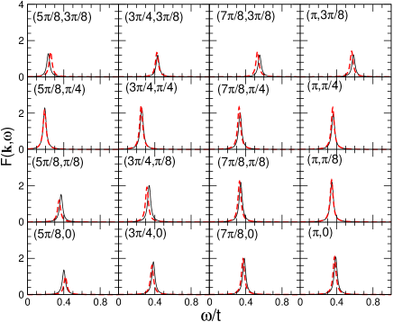
Figure 2: (Color online) The one-particle anomalous excitation spectrum $F({\bf k},\omega)$ for the projected BCS states [Eq. (10)] (solid lines). $|\Psi_{0}^{(N)}\rangle$ used here is optimized for the 2D $t$-$t^{\prime}$-$J$ model with $t^{\prime}/t=-0.2$, $J/t=0.3$, and $N=222$ on an $L=16\times 16$ cluster $(n\approx 0.87)$ with periodic boundary conditions note3 . The momenta ${\bf k}$ studied are indicated in the figures. For comparison, $F({\bf k},\omega)$ for a renormalized BCS theory (see the text) is also presented by dashed lines. The momentum-independent renormalization factor $z_{B}$ is 0.30. The delta function $\delta(\omega)$ is represented by a Lorentzian function $\varepsilon/{\pi(\omega^{2}+\varepsilon^{2})}$ with $\varepsilon=0.02t$.

To understand the nature of the low-lying excitations observed in $F({\bf k},\omega)$, here the results are analyzed based on a renormalized BCS theory with $d$-wave pairing symmetry text . The procedure adopted is as follows: (i) the excitation energy $E({\bf k})=E_{\bf k}^{(N+1)}-E_{0}^{(N)}$ is fitted for all momenta ${\bf k}$ in the whole Brillouin zone by a standard Bogoliubov excitation spectrum note6 , (ii) using the fitting parameters determined in (i), the BCS spectral weight for the one-particle anomalous excitations, ${u^{\rm(BCS)}_{\bf k}}^{*}v^{\rm(BCS)}_{\bf k}$, is calculated, and (iii) the BCS spectrum is renormalized by a momentum independent constant $z_{B}$ in such a way that

$$\sum_{\bf k}\left|Z_{2}^{(N)}({\bf k})\right|^{2}=z_{B}^{2}\sum_{\bf k}\left|u^{\rm(BCS)}_{\bf k}\cdot v^{\rm(BCS)}_{\bf k}\right|^{2}.$$ (11)

The obtained renormalized BCS spectra are shown in Fig. 2 by dashed lines. It is clearly seen in Fig. 2 that the renormalized BCS spectra can reproduce almost quantitatively $F({\bf k},\omega)$ for the projected BCS states. It should be emphasized that the procedure employed above is highly nontrivial and it is beyond a simple fitting of numerical data. Similar agreement is also found for different sets of model parameters, one of which is exemplified in Fig. 3. The surprisingly excellent agreement found here strongly indicates that the low-lying excitations described by the projected BCS states can be well understood within a renormalized Bogoliubov quasi-particle picture.

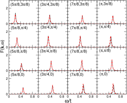
Figure 3: (Color online) The same as in Fig. 2 but for $N=240$ $(n\approx 0.94)$ note3 . The momentum-independent renormalization factor $z_{B}$ is 0.18.

To further examine the validity of the renormalized Bogoliubov quasi-particle picture for the projected BCS states, let us finally study the superconducting order parameter, which is here defined as $\Psi=\langle\psi_{0}^{(N+2)}|c_{{\bf i}\uparrow}^{\dagger}c_{{\bf i}+{\bf x}\downarrow}^{\dagger}|\psi_{0}^{(N)}\rangle$ (${\bf x}$ being the unit vector in the $x$ direction). The electron density ($n$) dependence of $\Psi$ is shown in Fig. 1 (c) for the 2D $t$-$t^{\prime}$-$J$ model, where $|\psi_{0}^{(N)}\rangle$ is optimized for each $n$ note3 . As seen in Fig. 1 (c), $|\Psi|^{2}$ vs $n$ shows a domelike behavior, similar to the pairing correlation function at the maximum distance as a function of $n$ reported before rand . It is also interesting to notice that $|\Psi|^{2}$ is proportional to $1-n$ for small $1-n$. The corresponding quantity $\Psi_{\rm BCS}$ for the BCS state with ${u^{\rm(BCS)}_{\bf k}}$ and $v^{\rm(BCS)}_{\bf k}$, determined by the procedure mentioned above, can also be calculated by $\Psi_{\rm BCS}={\frac{1}{L}}\sum_{\bf k}{\rm e}^{i{\bf k}\cdot{\bf x}}{u^{\rm(BCS)}_{\bf k}}^{*}v^{\rm(BCS)}_{\bf k}$. If a renormalized Bogoliubov quasi-particle picture is valid, $\Psi\cong z_{B}\Psi_{\rm BCS}$ is expected. As seen in Fig. 1 (c), this is in fact clearly the case. This result also gives a clear physical meaning to the renormalization factor $z_{B}$ introduced in Eq. (11).

As is well known, a Gutzwiller-projected Fermi gas is described within a Fermi liquid picture voll . The present results thus strongly suggest that analogously a Gutzwiller-projected, correlated BCS state (“projected BCS gas”) can still be described within a renormalized BCS-Bogoliubov quasi-particle picture (“BCS liquid”) note4 . This is in fact in accordance with recent photoemission spectroscopy experiments on high-$T_{\rm C}$ cuprate superconductors for which low-lying excitations consistent with a BCS theory have been revealed takahashi . Moreover, the present results would also provide a theoretical justification for employing a mean-field-based BCS-like theory to analyze the low-energy dynamics observed experimentally in the superconducting state of high-$T_{\rm C}$ cuprate superconductors bala .

To summarize, the one-particle anomalous excitations have been studied to understand the nature of the low-lying excitations of strongly correlated superconductors described by the Gutzwiller-projected BCS states. It was found that the low-lying excitations, which are highly coherent, can be essentially described within a renormalized Bogoliubov quasi-particle picture. This finding thus resembles the well-known result that a Gutzwiller-projected Fermi gas is a Fermi liquid. Finally, the present study has demonstrated that a variational Monte Carlo-based approach can be also utilized to explore low-lying excitations, and hopefully this work will stimulate further studies in this direction for other dynamical quantities.

The author would like to acknowledge useful discussion with S. Sorella, T. K. Lee, D. Ivanov, E. Dagotto, C.-P. Chou, S. Bieri, R. Hlubina, and S. Maekawa. This work was supported in part by INFM.

References

- (1) J. G. Bednorz and K. A. Müller, Z. Phys. B 64, 189 (1986).
- (2) For a recent review, see, e.g., P. A. Lee, N. Nagaosa, and X.-G. Wen, Rev. Mod. Phys. 78, 18 (2006), and references therein.
- (3) P. W. Anderson, Science 235, 1196 (1987).
- (4) C. Gros, Ann. Phys. (N.Y.) 189, 53 (1989); H. Yokoyama and M. Ogata, J. Phys. Soc. Jpn. 65, 3615 (1996), and references therein.
- (5) A. Paramekanti, M. Randeria, and N. Trivedi, Phys. Rev. Lett. 87, 217002 (2001); Phys. Rev. B 70, 054504 (2004).
- (6) S. Yunoki, E. Dagotto, and S. Sorella, Phys. Rev. Lett. 94, 037001 (2005).
- (7) N. Fukushima, B. Edegger, V. N. Muthukumar, and C. Gros, Phys. Rev. B72, 144505 (2005).
- (8) H.-Y. Yang, F. Yang, Y.-J. Jiang, and T. Li, cond-mat/0604488 (unpublished).
- (9) G. Senatore and N. H. March, Rev. Mod. Phys. 66, 445 (1994).
- (10) B. J. Powell and R. H. McKenzie, Phys. Rev. Lett. 94, 047004 (2005); J. Liu, J. Schmalian, and N. Trivedi, Phys. Rev. Lett. 94, 127003 (2005).
- (11) V.W. Scarola and S. Das Sarma, Phys. Rev. Lett. 95, 033003 (2005); T. Kimura, S. Tsuchiya, and S. Kurihara, Phys. Rev. Lett. 94, 110403 (2005).
- (12) See, e.g., D. Vollhardt, Rev. Mod. Phys. 56, 99 (1984).
- (13) See, e.g., J. R. Schrieffer, Theory of Superconductivity (Addison-Wesley, New York, 1988).
- (14) F. C. Zhang, C. Gros, T. M. Rice, and H. Shiba, Supercond. Sci. Technol. 1, 36 (1988).
- (15) P. W. Anderson and N. P. Ong, cond-mat/0405518 (unpublished).
- (16) S. Yunoki, Phys. Rev. B72, 092505 (2005).
- (17) Y. Ohta, T. Shimozato, R. Eder, and S. Maekawa, Phys. Rev. Lett. 73, 324 (1994).
- (18) P. Nozières, Theory of Interacting Fermi Systems (Addison-Wesley, New York, 1987), Chapt. 4.
- (19) A similar idea has also been pointed out independently by C.-P. Chou, T. K. Lee, and C.-M. Ho, Phys. Rev. B74, 092502 (2006), and by S. Bieri and D. Ivanov Phys. Rev. B75, 035104(2007).
- (20) It was found numerically that can also reproduce almost exactly, as expected for relatively large clusters.
- (21) Here the variational parameters are the nearest neighbor singlet gap function with -wave pairing symmetry, chemical potential , and the nearest neighbor hopping , i.e., with and . The optimized variational parameters are, for example, , , and for , and , , and for .
- (22) M. Randeria, R. Sensarma, N. Trivedi, and F.-C. Zhang, Phys. Rev. Lett. 95, 137001 (2005).
- (23) E. Dagotto and J. Riera, Phys. Rev. Lett. 70, 682 (1993); S. Sorella, G. B. Martins, F. Becca, C. Gazza, L. Capriotti, A. Parola, and E. Dagotto , Phys. Rev. Lett. 88, 117002 (2002); C. T. Shih, T. K. Lee, R. Eder, C.-Y. Mou, and Y. C. Chen, Phys. Rev. Lett. 92 227002 (2004).
- (24) E. Dagotto, Rev. Mod. Phys. 66, 763 (1994)
- (25) The fitting parameters used here are hoppings (included up to the fourth nearest neighbors), singlet gap functions with -wave symmetry (up to the second nearest neighbors), and chemical potential. However, it was found that the results presented in Figs. 1(c), 2, and 3 do not depend strongly on the number of fitting parameters chosen. Note also that the number of independent points is 45 for an cluster.
- (26) Except for the limit of . See, e.g., M. Randeria, A. Paramekanti, and N. Trivedi, Phys. Rev. B69, 144509 (2004).
- (27) H. Matsui, T. Sato, T. Takahashi, S.-C. Wang, H.-B. Yang, H. Ding, T. Fujii, T. Watanabe, and A. Matsuda, Phys. Rev. Lett. 90, 217002 (2003).
- (28) See, for example, A. V. Balatsky, I. Vekhter, and J.-X. Zhu, Rev. Mod. Phys. 78, 373 (2006), and references therein.