Exchange-controlled single-electron-spin rotations in quantum dots

Abstract

We show theoretically that arbitrary coherent rotations can be performed quickly (with a gating time $\sim 1\,\mathrm{ns}$) and with high fidelity on the spin of a single confined electron using control of exchange only, without the need for spin-orbit coupling or ac fields. We expect that implementations of this scheme would achieve gate error rates on the order of $\eta\lesssim 10^{-3}$ in GaAs quantum dots, within reach of several known error-correction protocols.

The elementary building-blocks for universal quantum computing are a two-qubit entangling operation, such as the cnot-gate or $\sqrt{\mbox{\sc swap}}$-gate and arbitrary single-qubit rotations. For qubits based on single electron spins confined to quantum dots, Loss and DiVincenzo (1998) recent experiments have now achieved the two-qubit $\sqrt{\mbox{\sc swap}}$-gate Petta et al. (2005) and single-spin coherent rotations.Koppens et al. (2006) If these operations are to be used in a viable quantum information processor, they must be performed with a sufficiently small gate error per operation $\eta\ll 1$. The threshold values of $\eta$ required for effective quantum error correction depend somewhat on error models and the particular error-correction protocol, but current estimates are in the range $\eta<10^{-2}-10^{-4}$.Steane (2003); Knill (2005) To achieve these low error rates, new schemes must be developed to perform quantum gates quickly and accurately within the relevant coherence times.

Previous proposals Engel and Loss (2001) and recent implementations Koppens et al. (2006) for single-spin rotation have relied on ac magnetic fields to perform electron-spin resonance (ESR). In ESR, difficulties with high-power ac fields limit single-spin Rabi frequencies to values that are much smaller than the operation rates typically associated with two-qubit gates mediated by exchange.Petta et al. (2005) To circumvent these problems while still achieving fast coherent single-qubit rotations, there have been several proposals to use exchange or electric-field (rather than magnetic-field) control of electron spin states. These proposals aim to perform rotations on multiple-spin encoded qubits,Hanson and Burkard (2007); Kyriakidis and Burkard (2007) or require strong spin-orbit interaction, Rashba and Efros (2003); Stepanenko and Bonesteel (2004); Flindt et al. (2006); Golovach et al. (2006) coupling to excited orbital states,Tokura et al. (2006) or rapid pulsing of magnetic fields.Wu et al. (2004) Qubits encoded in two states having different orbital wave functions are susceptible to dephasing through fluctuations in the electric environment, even in the idle state.Coish and Loss (2005); Hu and Das Sarma (2006); Stopa and Marcus (2006) Proposals that make use of the spin-orbit interaction Rashba and Efros (2003); Stepanenko and Bonesteel (2004); Flindt et al. (2006); Golovach et al. (2006) are restricted to systems where the spin-orbit coupling is sufficiently strong, excluding promising architectures such as quantum dots made from Si:SiGe Friesen et al. (2003) and carbon nanotubes or graphene sheets.Mason et al. (2004); Gräber et al. (2006); Trauzettel et al. (2007) Sufficiently rapid pulsing of magnetic fields Wu et al. (2004) may not be feasible in GaAs, where the electron-spin coherence time is on the order of $\tau_{c}\sim 10\,\mathrm{ns}$.Koppens et al. (2005); Petta et al. (2005)

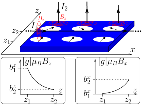
Figure 1: (Color online) Possible setup to implement the scheme proposed here. Ancillary electron spins at $z_{1}$ are maintained in a polarized state with a large Zeeman field $b_{1}^{z}$ along $z$. Qubit spins at $z_{2}$ are free to precess in a weaker effective Zeeman field lying in the $x$-$z$ plane: $\boldsymbol{\Delta}=(b_{2}^{x},0,b_{2}^{z}-J/2)$. Here, $J$ is the exchange coupling between the qubit and ancillary spins and $\mathbf{b}_{2}$ is the qubit Zeeman field in the absence of exchange. When $b_{1}^{z}\gg b_{2}^{z}\gg b_{2}^{x}$, $z$-rotations are performed if $J\approx 0$ and $x$-rotations are achieved when $J\approx 2b_{2}^{z}$.

Here we propose to perform single-qubit rotations in a way that would marry the benefits of demonstrated fast electrical control of the exchange interaction Petta et al. (2005) with the benefits of naturally long-lived single-electron spin qubits.Loss and DiVincenzo (1998) Our proposal would operate in the absence of spin-orbit coupling and would act on single electron spins without the use of ac electromagnetic fields, in the presence of a fixed Zeeman field configuration (Fig. 1). This scheme applies to confined electrons in any structure with a locally controllable potential. Specifically, this scheme may be applied to electrons above liquid helium, bound to gated phosphorus donors in silicon, and in quantum dots formed in a GaAs two-dimensional electron gas, nanowires, carbon nanotubes, or graphene.

Hamiltonian–We begin from a standard tunneling model for the two lowest orbital levels of a double quantum dot, including tunnel coupling $t_{12}$, on-site repulsion $U_{\mathrm{c}}$, nearest-neighbor repulsion $U^{\prime}_{\mathrm{c}}$, local electrostatic potentials $V_{1(2)}$ and a local Zeeman field $\mathbf{b}_{1(2)}$ on dot 1(2) (see Refs. [van der Wiel et al., 2003; Coish and Loss, 2006] and references therein):

$$\mathcal{H}=-\sum_{l\sigma}V_{l}n_{l\sigma}+U_{\mathrm{c}}\sum_{l}n_{l\uparrow}n_{l\downarrow}+U^{\prime}_{\mathrm{c}}\prod_{l}(n_{l\uparrow}+n_{l\downarrow})\\ +t_{12}\sum_{\sigma}\left(d_{1\sigma}^{\dagger}d_{2\sigma}+d_{2\sigma}^{\dagger}d_{1\sigma}\right)-\sum_{l}\mathbf{S}_{l}\cdot\mathbf{b}_{l}.$$ (1)

Here we have set $\hbar=1$, $d_{l\sigma}$ annihilates an electron in dot $l=1,2$ with spin $\sigma$, $n_{l\sigma}=d_{l\sigma}^{\dagger}d_{l\sigma}$ is the usual number operator, and $\mathbf{S}_{l}=\frac{1}{2}\sum_{s,s^{\prime}}c^{\dagger}_{ls}\boldsymbol{\sigma}_{s,s^{\prime}}c_{ls^{\prime}}$ is the spin density on dot $l$. We choose $|\epsilon\pm\delta b^{z}|\gg|t_{12}|$, $|\delta b^{z}|\gtrsim|t_{12}|$, with $\delta b^{z}=(b_{1}^{z}-b_{2}^{z})/2$ and $\epsilon=V_{2}-V_{1}-U_{\mathrm{c}}+U^{\prime}_{\mathrm{c}}$, which favors the $(1,1)$ charge state (where $(N_{1},N_{2})$ denotes a state with $N_{1(2)}$ electrons on dot 1(2), see Fig. 2). Additionally, we require a large Zeeman field along $z$ in dot 1 ($|b_{1}^{z}|\gg|b_{1}^{x,y}|$) so that the spin on dot 1 is frozen into its spin-up ground state. For simplicity, we furthermore choose $b_{2}^{y}=0$. Eq. (1) then reduces to the following low-energy effective Hamiltonian for the spin on dot 2:

$$\mathcal{H}_{\mathrm{eff}}=-\frac{1}{2}\boldsymbol{\Delta}\cdot\boldsymbol{\sigma};\;\boldsymbol{\Delta}=(b_{2}^{x},0,b_{2}^{z}-J(\epsilon)/2).$$ (2)

When $|\epsilon|\gg|\delta b^{z}|$, $J(\epsilon)\approx-2t_{12}^{2}/\epsilon$. Thus, for a fixed Zeeman field $\mathbf{b}_{2}$, the direction and magnitude of the effective field $\boldsymbol{\Delta}$ can be tuned with gate voltages via its dependence on $\epsilon$ (see Fig. 2(c)). Eq. (2) follows directly from a much more general Hamiltonian of the form $H=J(\epsilon)\mathbf{S}_{1}\cdot\mathbf{S}_{2}-\sum_{l}\mathbf{b}_{l}\cdot\mathbf{S}_{l}$ in the limit where $|\mathbf{b}_{1}|\gg|\mathbf{b}_{2}|,J$, and so this scheme is not limited to the particular Hamiltonian given in Eq. (1), which neglects the long-ranged nature of the Coulomb interaction and excited orbital states. The long-ranged part of the Coulomb interaction (the exchange integral) contributes a small fraction to $J(\epsilon)$ compared to the tunneling contribution when the out-of-plane magnetic field is zero Burkard et al. (1999) and contributions to $J(\epsilon)$ due to excited orbital states Stopa and Marcus (2006) are a small correction when $|\epsilon|<J_{(0,2)}$, where $J_{(0,2)}$ is the single-dot exchange coupling on dot 2. Outside of this range of validity, the functional form $J(\epsilon)$ could be obtained empirically, as has been done in Ref. [Laird et al., 2006].

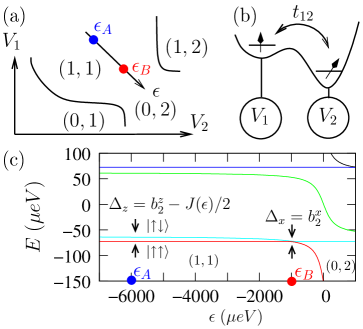
Figure 2: (Color online) (a) Charge stability diagram indicating the ground-state charge configuration $(N_{1},N_{2})$ for local dot potentials $V_{1},\,V_{2}$. In the $(1,1)$ configuration, the exchange interaction $J(\epsilon)$ can be tuned by shifting the double-dot potential difference $\epsilon\sim V_{2}-V_{1}$. (b) When the electron spin in dot 1 is polarized, the qubit electron acquires a Zeeman shift given by $t_{12}^{2}/\epsilon=-J(\epsilon)/2$ due to virtual hopping processes that are allowed for spin-down, but forbidden for spin-up due to the Pauli principle. (c) Energy spectrum of the Hamiltonian given in Eq. (1) in the presence of a strong inhomogeneous magnetic field.

Qubit gates–Arbitrary single-qubit rotations can be achieved with the appropriate composition of the Hadamard gate ($H$) and $\pi/8$ gate ($T$) Nielsen and Chuang (2001):

$$H=\frac{1}{\sqrt{2}}\left(\begin{array}[]{cc}1&1\\ 1&-1\end{array}\right),\;\;T=\left(\begin{array}[]{cc}1&0\\ 0&e^{i\pi/4}\end{array}\right).$$ (3)

Up to a global phase, $T$ corresponds to a rotation about $z$ by an angle $\phi=\pi/4$. This operation can be performed with high fidelity by allowing the qubit spin to precess coherently for a switching time $t_{\mathrm{s}}=\phi/\Delta_{z}$ at the operating point $\epsilon_{A}$ in Fig. 2(a), where $\Delta_{z}\gg\Delta_{x}$. The $H$ gate can be implemented by pulsing $\epsilon$ (see Fig. 2(c)) from $\epsilon_{A}$, where $\Delta_{z}\approx b_{2}^{z}$ to $\epsilon_{B}=-t_{12}^{2}/b_{2}^{z}$, where $\Delta_{z}\approx 0$ and back. The pulse is achieved with a characteristic rise/fall time $\tau$, and returns to $\epsilon=\epsilon_{A}$ after spending the pulse time $t_{\mathrm{p}}$ at $\epsilon=\epsilon_{B}$. If $b_{2}^{x}\ll b_{2}^{z}$, $\mathcal{H}_{\mathrm{eff}}$ induces approximate $z$-rotations during the rise/fall time, and $x$-rotations when $\epsilon=\epsilon_{\mathrm{B}}$. The entire switching process (with total switching time $t_{\mathrm{s}}=t_{\mathrm{p}}+4\tau$) is described by a time evolution operator $\mathcal{U}=\mathcal{T}e^{i\int_{0}^{t_{\mathrm{s}}}dt\boldsymbol{\Delta}(t)\cdot\boldsymbol{\sigma}/2}$, which, for $b_{2}^{x}\ll b_{2}^{z}$, is thus approximately given by

$$\mathcal{U}\approx\mathcal{U}(\phi_{x},\phi_{z})=R_{\hat{z}}\left(-\frac{\phi_{z}}{2}\right)R_{\hat{x}}\left(-\phi_{x}\right)R_{\hat{z}}\left(-\frac{\phi_{z}}{2}\right),$$ (4)

where $\phi_{x}=\Delta_{x}t_{\mathrm{p}}$ and $\phi_{z}=\int_{0}^{t_{\mathrm{s}}}dt\Delta_{z}(t)$. Here, $R_{\hat{n}}(\phi)$ is a rotation about the $\hat{n}$-axis by angle $\phi$. When $\phi_{x}=\pi/2$ and $\phi_{z}=\pi$, Eq. (4) gives an $H$ gate, up to a global phase: $\mathcal{U}(\pi/2,\pi)=iH$.

Errors–We quantify gate errors with the error rate $\eta=1-\mathcal{F}$, where $\mathcal{F}$ is the average gate fidelity, defined by

$$\mathcal{F}=\frac{1}{4\pi}\int d\Omega\overline{\mathrm{Tr}\left(U\rho_{\mathrm{in}}(\theta,\phi)U^{\dagger}\tilde{U}\rho_{\mathrm{in}}(\theta,\phi)\tilde{U}^{\dagger}\right)}.$$ (5)

Here, $\rho_{\mathrm{in}}(\theta,\phi)=\left|\theta,\phi\right>\left<\theta,\phi\right|$, where $\left|\theta,\phi\right>=\cos(\theta/2)\left|\uparrow\right>+e^{i\phi}\sin(\theta/2)\left|\downarrow\right>$ indicates an inital spin-1/2 coherent state in the qubit basis (the two-dimensional Hilbert space spanned by the (1,1) charge state and spin-up on dot 1), $U=H$ or $T$ is the ideal intended single-qubit gate operation, and $\tilde{U}=\mathcal{T}\exp{\left[-i\int_{0}^{t_{\mathrm{s}}}dt\mathcal{H}(t)\right]}$ is the true time evolution of the system under the time-dependent Hamiltonian $\mathcal{H}(t)$. The overbar indicates a Gaussian average over fluctuations in the classical Zeeman field $\mathbf{b}_{2}$, which reproduces the effects of hyperfine-induced decoherence due to an unknown static nuclear field when $\sigma\ll\left|\overline{\mathbf{b}_{2}}\right|$ Coish and Loss (2004):

$$\overline{f(\mathbf{b}_{2})}=\int\frac{d^{3}b_{2}}{\left(2\pi\sigma\right)^{3/2}}\exp\left(\frac{\left(\mathbf{b}_{2}-\overline{\mathbf{b}_{2}}\right)^{2}}{2\sigma^{2}}\right)f(\mathbf{b}_{2}).$$ (6)

For a gated lateral GaAs quantum dot, $\sigma_{N}^{2}=\overline{\left(\mathbf{b}_{2}-\overline{\mathbf{b}_{2}}\right)^{2}}=3\sigma^{2}$ due to hyperfine fluctuations has been measured, giving $\sigma_{N}=0.03\,\mu eV$.Koppens et al. (2005)

Based on the above protocol for gating operations, and assuming a coherence time $\tau_{c}$ for the qubit spins, a suitable parameter regime for high-fidelity single-qubit operations is given by the following hierarchy:

$$1/\tau_{c}\ll\overline{b_{2}^{x}}\ll\overline{b_{2}^{z}}\ll t_{12}\lesssim b_{1}^{z}\ll|\epsilon_{B}|<|\epsilon_{A}|.$$ (7)

The first inequality in Eq. (7) guarantees that $x$-rotations are achieved with high fidelity at the operating point $\epsilon=\epsilon_{B}$. The second inequality allows for high-fidelity $z$-rotations at $\epsilon=\epsilon_{A}$. The third and fourth inequalities are required to ensure that $\overline{b_{2}^{z}}$ can be cancelled by exchange $J\simeq 2t_{12}^{2}/\epsilon$, and the last two inequalities guarantee that the population of (0,2) (the double occupancy $D\simeq\left(t_{12}/\epsilon\right)^{2}$) remains small, which limits errors due to leakage and orbital dephasing (see below). When $\tau_{c}$ is dominated by hyperfine fluctuations, $1/\tau_{c}\sim\sigma_{N}$. In this case, we give a set of values for these parameters satisfying Eq. (7) in the caption of Fig. 3. The effective Zeeman-field gradient given here could be achieved under the following circumstances: (a) a GaAs double quantum dot with the nuclei in dot 1 at near full polarization, which would produce a maximum effective Zeeman splitting of $b_{1}^{z}\simeq 135\,\mu eV$ (high polarizations could be achieved, e.g., through optical pumping Imamoǧlu et al. (2003) or transport Rudner and Levitov (2006)), or (b) a nanomagnet neighboring a carbon nanotube or graphene double quantum dot with $g$-factor $g=2$ and inter-dot separation $\Delta L\sim 1\,\mu\mathrm{m}$ or an InAs nanowire double quantum dot with g-factor $g=8$ and inter-dot separation $\Delta L\sim 100\,\mathrm{nm}$, either of which would require a magnetic-field gradient on the order of $\Delta B/\Delta L\sim 1\mathrm{T}/\mu\mathrm{m}$. Comparable field gradients have already been achieved experimentally.Wróbel et al. (2004) Alternatively, the ancillary spins could be polarized with the exchange field from a neighboring ferromagnet, high $g$-factor material, or stripline currents (see Fig. 1). The values we have used for the detuning parameter $\epsilon$ and tunnel coupling $t_{12}$ are of the same order as those used in previous experiments. Petta et al. (2005)

Within the validity of the two-dimensional effective Hamiltonian $\tilde{U}\approx\exp{\left\{-i\mathcal{H}_{\mathrm{eff}}(\epsilon)t_{\mathrm{s}}\right\}}$, it is straightforward but tedious to calculate rotation errors at $\epsilon=\epsilon_{\mathrm{A}}$ ($z$-rotations: $U=R_{\hat{z}}(\phi)$) and $\epsilon=\epsilon_{\mathrm{B}}$ ($x$-rotations: $U=R_{\hat{x}}(\phi)$) using the expressions in Eqs. (5,6).

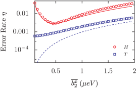
Figure 3: (Color online) Error rates for $H$ and $T$ gates. For these plots we have chosen the parameters $t_{12}=100\,\mu eV,\;b_{1}^{z}=135\,\mu eV$, $\overline{b_{2}^{z}}=10\,\mu eV,\;\overline{b_{2}^{x}}=1\,\mu eV$, and $\epsilon_{A}=-6\,\mathrm{m}eV$. For the Hadamard gate, these values result in $\epsilon_{B}=-t_{12}^{2}/\overline{b_{2}^{z}}=-1000\,\mu eV$, a pulse time $t_{\mathrm{p}}=\pi\hbar/2\overline{b_{2}^{x}}=1\,\mathrm{ns}$, and a rise/fall time $\tau\approx\pi\hbar/4\overline{b_{2}^{z}}=50\,\mathrm{ps}$. Symbols give the results of numerical integration of the time-dependent Schrödinger equation for the Hadamard gate ($H$, circles) and $\pi/8$ gate ($T$, squares). Lines give the estimates for gating error from Eq. (10).

The error rate for $z$-rotations is dominated by the misalignment of the average field $\overline{\mathbf{b}_{2}}$ with the $z$-axis and is thus small in the ratio $\overline{b_{2}^{x}}/\overline{b_{2}^{z}}$. For a rotation by angle $-\phi$ (to leading order in $\overline{b_{2}^{x}}/\overline{b_{2}^{z}}$), this error rate is

$$\eta^{z}(\phi)\approx\frac{2}{3}\left(\frac{\overline{b_{2}^{x}}}{\overline{b_{2}^{z}}}\right)^{2}\sin^{2}\left(\frac{\phi}{2}\right).$$ (8)

When $\overline{\Delta_{z}}=0$ (at $\epsilon=\epsilon_{\mathrm{B}}$), the error rate for $x$-rotations is dominated by hyperfine fluctuations, and is therefore small in $\sigma_{N}/\overline{b_{2}^{x}}$. We find this error rate for an $x$-rotation by angle $-\phi$ (to leading order in $\sigma_{N}/\overline{b_{2}^{x}}$) is

$$\eta^{x}(\phi)\approx\left(\frac{\phi^{2}}{18}+\frac{4}{9}\sin^{2}\left(\frac{\phi}{2}\right)\right)\left(\frac{\sigma_{N}}{\overline{b_{2}^{x}}}\right)^{2}.$$ (9)

We estimate the error in $T$ using $\eta^{z}(\phi)$ with $\phi=\pi/4$. To estimate the error in $H$, we use Eq. (4) in combination with Eqs. (8) and (9), assuming the errors incurred by each rotation are independent. These estimates give

$$\eta\approx\left\{\begin{array}[]{cc}\eta^{z}\left(\frac{\pi}{4}\right),&(U=T),\\ \eta^{x}\left(\frac{\pi}{2}\right)+2\eta^{z}\left(\frac{\pi}{2}\right),&(U=H).\end{array}\right.$$ (10)

From Eq. (10) we find the error rate for $H$ is always larger than that for $T$ and reaches a minimum at an optimal value of $\overline{b_{2}^{x}}$. The optimal value of $\overline{b_{2}^{x}}$ and $\eta$ at this point are:

$$b_{2}^{x,\mathrm{opt}}=\sqrt{C|\overline{b_{2}^{z}}|\sigma_{N}},\;\;\eta(b_{2}^{x,\mathrm{opt}})=\frac{4}{3}C\frac{\sigma_{N}}{|\overline{b_{2}^{z}}|},$$ (11)

where $C$ is a numerical prefactor $C=\sqrt{1/3+\pi^{2}/48}\simeq 0.73$. Using the measured value $\sigma_{N}=0.03\,\mu eV$ and $b_{2}^{z}=10\,\mu eV$, we find an optimized error rate of $\eta\sim 10^{-3}$. Here we have included the most dominant error mechanisms. There are many other potential sources of error, which we discuss in the following. All numerical estimates are based on the parameter values given in the caption of Fig 3.

The error due to leakage to the (0,2) singlet state or misalignment of $\mathbf{b}_{1}$ due to the hyperfine interaction in leading-order perturbation theory is given by $\sim\max\left[\left(\sigma_{N}/b_{1}^{z}\right)^{2},\left(t_{12}/\epsilon_{A}\right)^{2}\right]\sim 10^{-4}$.

If switching is done too slowly during the Hadamard gate, the qubit states will follow the adiabatic eigenbasis, introducing an additional source of error. We estimate this error to be $1-P\approx\alpha$, where $P=e^{-\alpha}$ is the Landau-Zeener tunneling probability, determined by Zener (1932)

$$\alpha=\frac{\pi|\overline{b_{2}^{x}}|^{2}}{|dJ(t)/dt|}\approx\frac{\pi|\overline{b_{2}^{x}}|^{2}\epsilon_{B}^{2}\tau}{2t_{12}^{2}|\Delta\epsilon|}\sim 10^{-4}.$$ (12)

Here, we have used $dJ(t)/dt\approx-2\dot{\epsilon}t_{12}^{2}/\epsilon_{B}^{2}$, with $|\dot{\epsilon}|\approx|\Delta\epsilon|/\tau$, where $\Delta\epsilon=\epsilon_{A}-\epsilon_{B}$. In the opposite limit, $\alpha\gg 1$, the qubit spin could be read out via charge measurements Petta et al. (2005) by sweeping slowly to large positive $\epsilon$, where the qubit state $\left|\uparrow\right>$ would be adiabatically converted to the (0,2) ground-state singlet, or initialized by sweeping in the opposite direction (see Fig. 2(c)).

In systems with finite spin-orbit coupling, the transverse-spin decay time $T_{2}$ is limited by the energy relaxation time $T_{1}$ (i.e., $T_{2}=2T_{1}$ Golovach et al. (2004)), so it is sufficient to analyze this error in terms of $T_{1}$. $T_{1}$ in quantum dots can now be measured,Elzerman et al. (2004) giving $T_{1}\sim 1\,\mathrm{ms}$ at fields of $B\approx 6\mathrm{T}$ ($g^{*}\mu_{B}B\simeq 135\,\mu eV$). Amasha et al. (2006) This value gives an error estimate on the order of $t_{\mathrm{s}}/T_{1}\lesssim 10^{-6}$ for a switching time $t_{\mathrm{s}}\simeq 1\,\mathrm{ns}$.

Finally, rapid voltage-controlled gating in this scheme is made possible only because the electron spin states are associated with different orbital wave functions during pulsing, which also makes these states susceptible to orbital dephasing. The associated dephasing time is, however, strongly suppressed in the limit where the double occupancy is small: $D\approx(t_{12}/\epsilon)^{2}\ll 1$. In particular, the dephasing time for the two-electron system is $\tau_{\phi}^{(2)}\gtrsim D^{-2}\tau_{\phi}^{(1)}$, Coish and Loss (2005) where $\tau_{\phi}^{(1)}\approx 1\,\mathrm{ns}$ Hayashi et al. (2003) is the single-electron dephasing time in a double quantum dot. This gives an error estimate of $t_{\mathrm{s}}/\tau_{\phi}^{(2)}\lesssim 10^{-4}$, using $t_{\mathrm{s}}\approx 1\,\mathrm{ns}$ and $D\sim 10^{-2}$ at the operating point $\epsilon=\epsilon_{B}$. It should be possible to further suppress orbital dephasing by choosing the operating point $\epsilon_{B}$ to coincide with a “sweet spot”, where $dJ(\epsilon_{B})/d\epsilon=0$. Coish and Loss (2005); Hu and Das Sarma (2006); Stopa and Marcus (2006)

Numerical analysis–To confirm the validity of the approximations made here and to verify the smallness of error mechanisms associated with leakage and finite pulse times, we have numerically integrated the time-dependent Schrödinger equation for the Hamiltonian given in Eq. (1) in the basis of the (0,2) singlet state and four (1,1) states (including spin). We have used the pulse scheme described following Eq. (3) and evaluated the gate error rates for $T$ and $H$ from the fidelity in Eq. (5). For the Hadamard gate we used the symmetric pulse shape

$$\epsilon(t)=\left\{\begin{array}[]{c}\epsilon_{0}+\frac{\Delta\epsilon}{2}\tanh\left(\frac{2\left[t-2\tau\right]}{\tau}\right),0<t<\frac{t_{\mathrm{s}}}{2}\\ \epsilon_{0}+\frac{\Delta\epsilon}{2}\tanh\left(\frac{2\left[t_{\mathrm{s}}-2\tau-t\right]}{\tau}\right),\frac{t_{\mathrm{s}}}{2}<t<t_{\mathrm{s}}\end{array}\right.,$$ (13)

where $\epsilon_{0}=\left(\epsilon_{A}+\epsilon_{B}\right)/2$ and $\Delta\epsilon=\epsilon_{B}-\epsilon_{A}$. The pulse time $t_{\mathrm{p}}$ and rise/fall time $\tau=(t_{\mathrm{s}}-t_{\mathrm{p}})/4$ were fixed using

$$t_{\mathrm{p}}=\frac{\pi}{2b_{2}^{x}},\;\;\pi=\int_{0}^{t_{\mathrm{s}}}\Delta_{z}(t)dt,$$ (14)

where the solution to the above integral equation was found numerically. The results of our numerics are shown in Fig. 3. To implement the integral (Eq. (6)) numerically, we have performed a Monte Carlo average over 100 Overhauser fields, sampled from a uniform Gaussian distribution using the experimental value $\sigma_{N}=0.03\,\mu eV$. Error bars due to the finite sample of Overhauser fields are smaller than the symbol size. We find good agreement between the analytical and predicted error rate for $T$ in the limit of large $\overline{b_{2}^{x}}$ (the saturation value for $\eta$ at low $\overline{b_{2}^{x}}$ is consistent with our estimates of $\sim 10^{-4}$ for error due to leakage). Additionally, we find reasonable agreement with our estimate for the $H$-gate error rate, confirming that we have identified the dominant error mechanisms. This gives us confidence that an error rate on the order of $\sim 10^{-3}$ should be achievable with this proposed scheme.

Acknowledgments–We thank G. Burkard, H.-A. Engel, M. Friesen, V. N. Golovach, J. Lehmann, D. Lidar, B. Trauzettel, and L. M. K. Vandersypen for useful discussions. We acknowledge financial support from JST ICORP, EU NoE MAGMANet, the NCCR Nanoscience, and the Swiss NSF.

References

- Loss and DiVincenzo (1998) D. Loss and D. P. DiVincenzo, Phys. Rev. A 57, 120 (1998).
- Petta et al. (2005) J. R. Petta, A. C. Johnson, J. M. Taylor, E. A. Laird, A. Yacoby, M. D. Lukin, C. M. Marcus, M. P. Hanson, and A. C. Gossard, Science 309, 2180 (2005).
- Koppens et al. (2006) F. H. L. Koppens, C. Buizert, K. J. Tielrooij, I. T. Vink, K. C. Nowack, T. Meunier, L. P. Kouwenhoven, and L. M. K. Vandersypen, Nature 442, 766 (2006).
- Steane (2003) A. M. Steane, Phys. Rev. A 68, 042322 (2003).
- Knill (2005) E. Knill, Nature 434, 39 (2005).
- Engel and Loss (2001) H.-A. Engel and D. Loss, Phys. Rev. Lett. 86, 4648 (2001).
- Hanson and Burkard (2007) R. Hanson and G. Burkard, Phys. Rev. Lett. 98, 050502 (2007).
- Kyriakidis and Burkard (2007) J. Kyriakidis and G. Burkard, Phys. Rev. B 75, 115324 (2007).
- Rashba and Efros (2003) E. I. Rashba and A. L. Efros, Phys. Rev. Lett. 91, 126405 (2003).
- Stepanenko and Bonesteel (2004) D. Stepanenko and N. E. Bonesteel, Phys. Rev. Lett. 93, 140501 (2004).
- Flindt et al. (2006) C. Flindt, A. S. Sørensen, and K. Flensberg, Phys. Rev. Lett. 97, 240501 (2006).
- Golovach et al. (2006) V. N. Golovach, M. Borhani, and D. Loss, Phys. Rev. B 74, 165319 (2006).
- Tokura et al. (2006) Y. Tokura, W. G. van der Wiel, T. Obata, and S. Tarucha, Phys. Rev. Lett. 96, 047202 (2006).
- Wu et al. (2004) L.-A. Wu, D. A. Lidar, and M. Friesen, Phys. Rev. Lett. 93, 030501 (2004).
- Coish and Loss (2005) W. A. Coish and D. Loss, Phys. Rev. B 72, 125337 (2005).
- Hu and Das Sarma (2006) X. Hu and S. Das Sarma, Phys. Rev. Lett. 96, 100501 (2006).
- Stopa and Marcus (2006) M. Stopa and C. M. Marcus, arXiv.org:cond-mat/0604008 (2006).
- Friesen et al. (2003) M. Friesen, P. Rugheimer, D. Savage, M. Lagally, D. van der Weide, R. Joynt, and M. Eriksson, Phys. Rev. B 67, 121301 (2003).
- Mason et al. (2004) N. Mason, M. J. Biercuk, and C. M. Marcus, Science 303, 655 (2004).
- Gräber et al. (2006) M. R. Gräber, W. A. Coish, C. Hoffmann, M. Weiss, J. Furer, S. Oberholzer, D. Loss, and C. Schönenberger, Phys. Rev. B 74, 075427 (2006).
- Trauzettel et al. (2007) B. Trauzettel, D. V. Bulaev, D. Loss, and G. Burkard, Nat. Phys. 3, 192 (2007).
- Koppens et al. (2005) F. H. L. Koppens, J. A. Folk, J. M. Elzerman, R. Hanson, L. H. W. van Beveren, I. T. Vink, H. P. Tranitz, W. Wegscheider, L. P. Kouwenhoven, and L. M. K. Vandersypen, Science 309, 1346 (2005).
- van der Wiel et al. (2003) W. G. van der Wiel, S. de Franceschi, J. M. Elzerman, T. Fujisawa, S. Tarucha, and L. P. Kouwenhoven, Rev. Mod. Phys. 75, 1 (2003).
- Coish and Loss (2006) W. A. Coish and D. Loss, arXiv:cond-mat/0606550 (2006), to appear in the Handbook of Magnetism and Advanced Magnetic Materials, vol. 5, eds. S. Parkin and D. Awschalom, Wiley.
- Burkard et al. (1999) G. Burkard, D. Loss, and D. P. DiVincenzo, Phys. Rev. B 59, 2070 (1999).
- Laird et al. (2006) E. A. Laird, J. R. Petta, A. C. Johnson, C. M. Marcus, A. Yacoby, M. P. Hanson, and A. C. Gossard, Phys. Rev. Lett. 97, 056801 (2006).
- Nielsen and Chuang (2001) M. A. Nielsen and I. L. Chuang, Quantum Computation and Quantum Information (Cambridge, 2001).
- Coish and Loss (2004) W. A. Coish and D. Loss, Phys. Rev. B 70, 195340 (2004).
- Imamoǧlu et al. (2003) A. Imamoǧlu, E. Knill, L. Tian, and P. Zoller, Phys. Rev. Lett. 91, 017402 (2003).
- Rudner and Levitov (2006) M. S. Rudner and L. S. Levitov, arXiv.org:cond-mat/0609409 (2006).
- Wróbel et al. (2004) J. Wróbel, T. Dietl, A. Łusakowski, G. Grabecki, K. Fronc, R. Hey, K. H. Ploog, and H. Shtrikman, Phys. Rev. Lett. 93, 246601 (2004).
- Zener (1932) C. Zener, Proc. Roy. Soc. Lond. 137, 696 (1932).
- Golovach et al. (2004) V. N. Golovach, A. Khaetskii, and D. Loss, Phys. Rev. Lett. 93, 016601 (2004).
- Elzerman et al. (2004) J. M. Elzerman, R. Hanson, L. H. Willems van Beveren, B. Witkamp, L. M. K. Vandersypen, and L. P. Kouwenhoven, Nature (London) 430, 431 (2004).
- Amasha et al. (2006) S. Amasha, K. MacLean, I. Radu, D. Zumbuhl, M. Kastner, M. Hanson, and A. Gossard, arXiv:cond-mat/0607110 (2006).
- Hayashi et al. (2003) T. Hayashi, T. Fujisawa, H. D. Cheong, Y. H. Jeong, and Y. Hirayama, Phys. Rev. Lett. 91, 226804 (2003).