Paired state in an integrable spin-1 boson model

Abstract

An exactly solvable model describing the low density limit of the spin-1 bosons in a one-dimensional optical lattice is proposed. The exact Bethe ansatz solution shows that the low energy physics of this system is described by a quantum liquid of spin singlet bound pairs. Motivated by the exact results, a mean-field approach to the corresponding three-dimensional system is carried out. Condensation of singlet pairs and coexistence with ordinary Bose-Einstein condensation are predicted.

I Introduction

Study on the trapped cold atoms opens the door for finding new matter states which are usually unknown or even do not exist in nature. Experimentally, the cold atom gas can be realized by means of either magnetic or optical traps. With Feshbach resonance, the scattering length and thus the couplings among atoms can be manipulated experimentally. In addition, with laser beams, one can confine particles in valleys of periodic potential of the optical lattice. These experimental tools provide a platform to study quite clean and controllable “artificial condensed matter systems”. Moreover, particles with higher inner degrees of freedom (hyperfine spin), which usually do not exist in conventional condensed matters, can be prepared by catching several hyperfine sublevels of atoms. Compared to spinless Bose gases, the low-energy physics of these systems such as the spin dynamicsdiener1 ; diener11 ; diener2 is much richer and may show fascinating macroscopic quantum phenomena. For example, the multi-component Bose-Einstein condensation (BEC) is realized in ${}^{87}Rb$ 1 and ${}^{23}Na$ 2 ; 3 ; 4 gases with optical traps. Both ${}^{87}Rb$ and ${}^{23}Na$ atoms have a hyperfine spin $F=1$. The interaction among ${}^{87}Rb$ atoms is ferromagnetic, which leads to a spin-polarized (ferromagnetic) ground state, while the spin exchange interaction among the ${}^{23}Na$ atoms is antiferromagnetic, leaving the ground state a spin singlet condensate. In an optical lattice, the Mott phase of $F=1$ cold atoms may exhibit rich magnetic structures. Nematic singlet 8 or dimerized 9 ground state has been proposed. Nevertheless, study on spinor cold atoms is still young and a quite interesting issue 10 ; 11 ; 12 ; 13 in modern many body physics.

In this Letter, we propose an exactly solvable model for $F=1$ bosonic cold atoms. The Bethe ansatz solution exactly shows that atoms may form spin singlet pairs with a finite energy gap and the low-energy physics is described by a quantum liquid of spin singlet atom pairs. Based on the exact solution for the 1D model, an appropriate mean-field theory is proposed to study the corresponding 3D systems. BCS-like pair condensation and coexistence with ordinary BEC are found in the 3D model.

II The model

In an optical lattice, it has been proposed that the following boson Hubbard model boson1 ; boson2 well describes the low-energy physics of the spinor bosons:

$$H= - t\sum_{<i,j>,s}(a_{i,s}^{\dagger}a_{j,s}+h.c.)+\frac{U_{0}}{2}\sum_{i}n_{i}(n_{i}-1)$$ (1)

$$+ \frac{U_{2}}{2}\sum_{i}({\bf S}_{i}^{2}-2n_{i})-\mu\sum_{i}n_{i},$$

where $a_{i,s}^{\dagger}$ ($a_{i,s}$) is the creation (annihilation) operator of atoms on site $i$ with spin index $s$, $n_{i}$ and ${\bf S}_{i}$ are the particle number and spin operators, respectively; $\mu$ is the chemical potential.

Recently, tremendous experimental and theoretical progress has been achieved in realization of one-dimensional (1D) cold atom systems a ; h ; h1 ; b ; t ; bl and 2D systemsre . The Mott phase diagram of $F=1$ bosons in an optical lattice has been given in ref.13 . In the metallic phase, it is known that the 1D spinless bosonic atom gases are well described by Lieb-Liniger model lieb ; lieb1 and several physical properties based on Lieb-Liniger’s exact results have been derivedfuchs ; liebseir . However, results on 1D cold atoms with internal degrees of freedom in the metallic phase are still rare. Generally speaking, a 1D exactly solvable model not only gives the best understanding for the corresponding universal class, but also provides some useful clues for understanding three-dimensional (3D) systems.

In this paper, instead of studying model (1), we consider the following 1D Hamiltonian:

$$H=-\sum_{i=1}^{N}\frac{\partial^{2}}{\partial x_{i}^{2}}+\sum_{i<j}[c_{0}+c_{2}{\bf S}_{i}\cdot{\bf S}_{j}]\delta(x_{i}-x_{j}),$$ (2)

where ${\bf S}_{i}$ is the spin operator with $z$-components $s=\uparrow,0,\downarrow$; $c_{0}=(g_{0}+2g_{2})/3$, $c_{2}=(g_{2}-g_{0})/3$, $g_{S}=4\pi\hbar^{2}l_{S}/M_{b}$, $M_{b}$ is the mass of boson and $l_{S}$ is the $s$-wave scattering length in the total spin $S$ channel diener1 ; diener11 . In the second quantization form, we define the particle creation (annihilation) operators as $a_{s}^{\dagger}(x)$ ($a_{s}(x)$). Obviously, the model (2) is just the low density limit of the boson Hubbard model (1). We note that two-particle scattering processes keep the conservation of the total spin $S$ and therefore the model possesses an $SU(2)$ invariance. Non-trivial scattering occurs only in the $S=0$ and $S=2$ channels. In the $S=1$ channel the wave-function is antisymmetric by exchanging two particles and the delta-function interaction is irrelevant. Especially in the $S=0$ channel, a special scattering process

$$a_{\uparrow}^{\dagger}(x)+a_{\downarrow}^{\dagger}(x)\to 2a_{0}^{\dagger}(x)$$ (3)

occurs, which makes the total particle number of an individual spin component is no longer a good quantum number and breaks the $SU(3)$ invariance. It is easy to verify that the present model has the following conserved quantities:

$$N = \sum_{s}\int a_{s}^{\dagger}(x)a_{s}(x)dx,$$

$$S^{z} = \int[a_{\uparrow}^{\dagger}(x)a_{\uparrow}(x)-a_{\downarrow}^{\dagger}(x)a_{\downarrow}(x)]dx,$$ (4)

where ${N}$ and $S^{z}$ are the total particle number operator and $z$-component of the total spin operator, respectively. Because of the $SU(2)$ invariance of the Hamiltonian, there are also two other good quantum numbers:

$$S^{+}=\sqrt{2}\int[a_{\uparrow}^{\dagger}(x)a_{0}(x)+a_{0}^{\dagger}(x)a_{\downarrow}(x)]dx,$$

$$S^{-}=\sqrt{2}\int[a_{0}^{\dagger}(x)a_{\uparrow}(x)+a_{\downarrow}^{\dagger}(x)a_{0}(x)]dx.$$ (5)

${S^{z}}$ and ${S^{\pm}}$ form the generators of the $SU(2)$ algebra. These three spin operators, combined with the five spin quadrupole operators

$$Q_{0} = \int[a^{\dagger}_{\uparrow}(x)a_{\uparrow}(x)+a^{\dagger}_{\downarrow}(x)a_{\downarrow}(x)-2a_{0}^{\dagger}(x)a_{0}(x)]dx,$$

$$Q_{2} = \int[a^{\dagger}_{\uparrow}(x)a_{\downarrow}(x)+a^{\dagger}_{\downarrow}(x)a_{\uparrow}(x)]dx,$$

$$Q_{xy} = -i\int[a^{\dagger}_{\uparrow}(x)a_{\downarrow}(x)-a^{\dagger}_{\downarrow}(x)a_{\uparrow}(x)]dx,$$ (6)

$$Q_{xz} = \frac{1}{\sqrt{2}}\int[a_{\uparrow}^{\dagger}(x)a_{0}(x)-a_{0}^{\dagger}(x)a_{\downarrow}(x)+h.c.]dx,$$

$$Q_{yz} = -\frac{i}{\sqrt{2}}\int[a_{\uparrow}^{\dagger}(x)a_{0}(x)-a_{0}^{\dagger}(x)a_{\downarrow}(x)-h.c.]dx,$$

form the basic representation of the $SU(3)$ algebra.

III Bethe Ansatz Solution

The pioneer work on the integrable models with internal degrees of freedom was done by Yangyang ; yang1 and followed by Sutherlandyang3 . There are two integrable lines for the model (2). The first is the $c_{2}=0$ case, i.e., $SU(3)$-invariant case, which has been solved by Sutherlandyang3 . The second integrable line is $c_{0}=c_{2}$, which has never been studied before and is the main target of the present work. In the framework of coordinate Bethe ansatz, the wave function of the system described by a set of quasi-momenta $\{k_{j}\}$ can be written asyang ; yang1

$$\Psi(x_{1}s_{1},\cdots,x_{N}s_{N})=\sum_{Q,P}\theta(x_{Q_{1}}<\cdots<x_{Q_{N}})$$

$$\quad\quad\times A_{s_{1}\cdots s_{N}}(Q,P)e^{i\sum_{l=1}^{N}k_{P_{l}}x_{Q_{l}}},$$ (7)

where $Q=(Q_{1},\cdots,Q_{N})$ and $P=(P_{1},\cdots,P_{N})$ are the permutations of the integers $1,\cdots,N$, $\theta(x_{Q_{1}}<\cdots<x_{Q_{N}})=\theta(x_{Q_{N}}-x_{Q_{N-1}})\cdots\theta(x_{Q_{2}}-x_{Q_{1}})$ and $\theta(x-y)$ is the step function. The wave function is symmetric under permutating both the coordinates and the spins of two atoms. The wave function is continuous but its derivative jumps when two atoms touch. With the standard coordinate Bethe ansatz procedure, we obtain the two-body scattering matrix for $c_{0}=c_{2}=c$ as

$$S_{ij}=\frac{k_{i}-k_{j}-ic}{k_{i}-k_{j}+ic}P_{ij}^{0}+P_{ij}^{1}+\frac{k_{i}-k_{j}+2ic}{k_{i}-k_{j}-2ic}P_{ij}^{2},$$ (8)

where $P_{ij}^{S},{~{}~{}}S=0,1,2$ is the spin projection operator onto the state of total spin $S$. The scattering matrix satisfies the Yang-Baxter equationyang ; yang1 ; yang3

$$S_{12}(k_{1}-k_{2})S_{13}(k_{1}-k_{3})S_{23}(k_{2}-k_{3})$$

$$\quad=S_{23}(k_{2}-k_{3})S_{13}(k_{1}-k_{3})S_{12}(k_{1}-k_{2}),$$ (9)

which ensures the integrability of the model (2) at $c_{0}=c_{2}=c$. With the periodic boundary conditions of the wave function, we obtain the following eigenvalue equations

$$S_{jN}S_{jN-1}\cdots S_{jj+1}S_{jj-1}\cdots S_{j1}e^{ik_{j}L}\xi_{0}=\xi_{0},$$ (10)

where $\xi_{0}$ is the amplitude of initial state wave function. We follow the algebraic Bethe ansatz method developed in babujian ; babujian1 ; schlottmann to solve the above eigenvalue problem. In fact, the $S$-matrix of the present model has the same structure to that of the $R$-operator of the Takhtajan-Babujian modelbabujian ; babujian1 . In such a sense, the spin dynamics of our model keeps some similarity to that of the Takhtajan-Babujian spin chain. Firstly, we define the monodromy matrix as

$${\cal T_{0}}(\lambda) = S_{0j}S_{0N}S_{0N-1}\cdots S_{0j+1}S_{0j-1}\cdots S_{01}$$ (14)

$$= \left(\begin{array}[]{ccc}A_{1}(\lambda)&B_{1}(\lambda)&B_{2}(\lambda)\\ C_{1}(\lambda)&A_{2}(\lambda)&B_{3}(\lambda)\\ C_{2}(\lambda)&C_{3}(\lambda)&A_{3}(\lambda)\end{array}\right),$$

where $S_{0l}\equiv S_{0l}(\lambda-k_{l})$. The eigenvalue problem (10) is therefore reduced to

$$tr_{0}{\cal T_{0}}(k_{j})e^{ik_{j}L}\xi_{0}=\xi_{0}.$$ (15)

The monodromy matrix satisfies the Yang-Baxter relation

$$S_{12}(\lambda-u){\cal T}_{1}(\lambda){\cal T}_{2}(u)={\cal T}_{2}(u){\cal T}_{1}(\lambda)S_{12}(\lambda-u).$$ (16)

Further, we define an auxiliary monodromy matrix as

$$T(\lambda) = S_{0j}^{\sigma s}S_{0N}^{\sigma s}\cdots S_{0j+1}^{\sigma s}S_{0j-1}^{\sigma s}S_{01}^{\sigma s}$$ (19)

$$= \left(\begin{array}[]{cc}A(\lambda)&B(\lambda)\\ C(\lambda)&D(\lambda)\end{array}\right),$$

with

$$S_{0l}^{\sigma s}(\lambda)=\frac{\lambda-k_{l}-i\frac{1}{2}c-ic{\bf\sigma}_{0}\cdot{\bf S}_{l}}{\lambda-k_{l}+i\frac{3}{2}c}.$$ (20)

The monodromy matrices (14) and (19) satisfy the Yang-Baxter relations

$$S_{12}^{\sigma s}(\lambda-u)T_{1}(\lambda){\cal T}_{2}(u)={\cal T}_{2}(u)T_{1}(\lambda)S_{12}^{\sigma s}(\lambda-u),$$

$$S_{12}^{\sigma\sigma}(\lambda-\mu)T_{1}(\lambda)T_{2}(\mu)=T_{2}(\mu)T_{1}(\lambda)S_{12}^{\sigma\sigma}(\lambda-\mu),$$ (21)

with $S_{12}^{\sigma\sigma}(\lambda)=(\lambda-ic)^{-1}(\lambda-ic/2-ic{\bf\sigma}_{1}\cdot{\bf\sigma}_{2}/2)$. From Eq. (21) we obtain the following commutation relations

$$A_{1}(\lambda)B(u)=\frac{\lambda-u+i\frac{3}{2}c}{\lambda-u-i\frac{1}{2}c}B(u)A_{1}(\lambda)$$

$$-\frac{i\sqrt{2}c}{\lambda-u-i\frac{1}{2}c}B_{1}(\lambda)A(u),\hskip 28.45274pt$$ (22)

$$A_{2}(\lambda)B(u)=\frac{(\lambda-u+i\frac{3}{2}c)(\lambda-u-i\frac{3}{2}c)}{(\lambda-u+i\frac{1}{2}c)(\lambda-u-i\frac{1}{2}c)}B(u)A_{2}(\lambda)$$

$$+\frac{i\sqrt{2}c}{\lambda-u-i\frac{1}{2}c}B_{1}(\lambda)D(u)-\frac{i\sqrt{2}c}{\lambda-u+i\frac{1}{2}c}B_{3}(\lambda)A(u)$$

$$+\frac{2ic}{(\lambda-u+i\frac{1}{2}c)(\lambda-u-i\frac{1}{2}c)}B_{2}(\lambda)C(u),\hskip 44.10185pt$$ (23)

$$A_{3}(\lambda)B(u)=\frac{\lambda-u-i\frac{3}{2}c}{\lambda-u+i\frac{1}{2}c}B(u)A_{3}(\lambda)$$

$$+\frac{i\sqrt{2}c}{\lambda-u+i\frac{1}{2}c}B_{3}(\lambda)D(u).\hskip 28.45274pt$$ (24)

Meanwhile, the commutation relations of $A(\lambda)$, $D(\lambda)$ and $B(\lambda)$ read

$$A(\lambda)B(u)=\frac{\lambda-u+ic}{\lambda-u}B(u)A(\lambda)-\frac{ic}{\lambda-u}B(\lambda)A(u),$$ (25)

$$D(\lambda)B(u)=\frac{\lambda-u-ic}{\lambda-u}B(u)D(\lambda)+\frac{ic}{\lambda-u}B(\lambda)D(u).$$ (26)

The vacuum state of the system is defined as $|\Omega\rangle=|\uparrow\rangle_{1}\otimes\cdots\otimes|\uparrow\rangle_{N}$. It is a common eigenstate of $A_{1}(\lambda)$, $A_{2}(\lambda)$, $A_{3}(\lambda)$, $A(\lambda)$ and $D(\lambda)$. The element $C(\lambda)$ acting on the vacuum state gives zero. The element $B(\lambda)$ acting on the vacuum state gives nonzero values and thus can be regarded as generating operator of eigenstates

$$|\Psi\rangle=B(u_{1})\cdots B(u_{M})|\Omega\rangle.$$ (27)

$tr_{0}{\cal T}(k_{j})\equiv\sum_{n=1}^{3}A_{n}(k_{j})$ acting on the assumed Bethe states (27) gives two kinds of terms, i.e., wanted and unwanted terms. Putting the unwanted terms to be zero we readily obtain the following Bethe ansatz equations for the rapidities $\{k_{j}\}$,

$$e^{ik_{j}L}=\prod_{l=1,l\neq j}^{N}\frac{k_{j}-k_{l}+2ic}{k_{j}-k_{l}-2ic}\prod_{\alpha=1}^{M}\frac{k_{j}-\Lambda_{\alpha}-ic}{k_{j}-\Lambda_{\alpha}+ic},$$ (28)

$$\prod_{l=1}^{N}\frac{\Lambda_{\alpha}-k_{l}-ic}{\Lambda_{\alpha}-k_{l}+ic}=-\prod_{\beta=1}^{M}\frac{\Lambda_{\alpha}-\Lambda_{\beta}-ic}{\Lambda_{\alpha}-\Lambda_{\beta}+ic},\hskip 28.45274pt$$ (29)

where $j,l=1,\cdots,N$, $\alpha,\beta=1,\cdots,M$, $M$ is the number of flipped spins and $\{\Lambda_{\alpha}\}$ is the set of the spin rapidities. The corresponding eigenvalue of the Hamiltonian (2) reads

$$E=\sum_{j=1}^{N}k_{j}^{2}.$$ (30)

IV Thermodynamic limit

Above we have confined the particles in a finite 1D box with length $L$. Based on the solutions of the Bethe ansatz equations, we can study the ground state and low-temperature properties of the system in the thermodynamic limit $L\to\infty$, $N/L\to n$. The solutions of the Bethe ansatz equations are a little bit complicated. Besides real solutions of $\{k_{j}\},{~{}}\{\Lambda_{\alpha}\}$, Eqs. (28-29) have also complex solutions for both $c>0$ and $c<0$, which are usually called as string solutions. For $c>0$, attractive interaction only occurs in the $S=0$ channel. That means particles may form spin singlet bound pairs. Generally, the complex solutions are determined by the poles or zeros of the Bethe ansatz equations in the thermodynamic limit. For example, if some $k_{j}$ in the upper complex plane, the left side of Eq. (28) tends to zero when $L\to\infty$. Correspondingly, there must exist a $\Lambda_{\alpha}$ satisfying $k_{j}-\Lambda_{\alpha}-ic\to 0$. Furthermore, from Eq. (29) we learn that there is another $\Lambda_{\beta}$ with $\Lambda_{\alpha}-\Lambda_{\beta}+ic\to 0$. For the complex conjugate invariance of the equations, we obtain the simple conjugate $k_{j}$-pair solutions

$$k_{j} = K_{j}+ic/2+o(e^{-\delta L}),$$

$$k_{j}^{*} = K_{j}-ic/2+o(e^{-\delta L}),$$ (31)

associated with $\Lambda$ 2-strings

$$\Lambda_{j} = K_{j}+ic/2+o(e^{-\delta^{\prime}L}),$$

$$\Lambda_{j}^{*} = K_{j}-ic/2+o(e^{-\delta^{\prime}L}),$$ (32)

where $K_{j}$ is a real parameter, $\delta$ and $\delta^{\prime}$ are some positive constants. We studied the 3 and 4-particle cases and verified that Eq. (31) describes the only possible bound state in the charge sector. In fact, no more than two atoms can form a bound state because of the symmetry constraint of the wave functions. In the thermodynamic limit, each bound pair contributes bound energy $\Delta=c^{2}/2$. Therefore, the low energy physics of the present system must be described by a quantum liquid of these bound pairs. In the ground state, all particles form such kind of bound pairs (Even $N$ is supposed. For odd $N$, there is a single unpaired particle and the ground state is 3-fold degenerate). Substituting these 2-string ansatz into Eqs. (28-29) and taking logarithm, we arrive at one set of reduced Bethe ansatz equations

$$K_{j}L=\pi I_{j}-\sum_{l=1,l\neq j}^{N}\left[\arctan\left(\frac{2(K_{j}-K_{l})}{3c}\right)\right.\quad\quad$$

$$\left.+\arctan\left(\frac{K_{j}-K_{l}}{c}\right)-\arctan\left(\frac{2(K_{j}-K_{l})}{c}\right)\right],$$ (33)

where $I_{j}$ is integer (half integer) for $N/2$ odd (even). The ground state corresponds to a sequence of consecutive $I_{j}$’s around zero symmetrically. In the thermodynamic limit,define $\rho_{0}(K_{j})=L^{-1}(I_{j+1}-I_{j})/(K_{j+1}-K_{j}))$ as the density of flipped spins. Taking derivative of Eq. (33), we obtain that the density distribution $\rho_{0}(K)$ in the ground state satisfies the following integral equation

$$\rho_{0}(K)=\frac{1}{\pi}+\frac{1}{\pi}\int_{-Q}^{Q}\left[\frac{6|c|}{9c^{2}+4(K-K^{\prime})^{2}}\right.\hskip 42.67912pt$$

$$\left.+\frac{|c|}{c^{2}+(K-K^{\prime})^{2}}-\frac{2|c|}{4c^{2}+(K-K^{\prime})^{2}}\right]\rho_{0}(K^{\prime})dK^{\prime},$$ (34)

where the pseudo Fermi point $Q$ is determined by

$$n=2\int^{Q}_{-Q}\rho_{0}(K)dK.$$ (35)

The density of the ground state energy reads

$$\frac{E_{0}}{L}=\int_{-Q}^{Q}\left(2K^{2}-\frac{c^{2}}{2}\right)\rho_{0}(K)dK.$$ (36)

Obviously, the ground state is a global spin singlet with $S^{z}=N-M=0$. However, it is not an $SU(3)$ singlet state. In the insulator phase of the boson-Hubbard model, a spin nematic state or a spin quadrupole polarized state zhang has been obtained. In our case, the spin part of the wave function of each bound pair takes the form $(|\uparrow,\downarrow\rangle+|\downarrow,\uparrow\rangle-|0,0\rangle)/\sqrt{3}$. It can be easily deduced that the expectation values of the quadrupole momenta per unit length are $\langle Q_{0}\rangle=-n/2$ and $\langle Q_{\alpha}\rangle=0$ for $\alpha\neq 0$. There is a finite energy gap $\Delta=c^{2}/2$ for the spin excitations. The only basic gapless excitation is in the charge sector. This can be realized by either digging a hole in the $K$ pseudo Fermi sea or putting a particle above the pseudo Fermi point (Note we treat an atom pair as a single particle here). The excitation energy $\epsilon(K)$ of a hole or a particle with quasi momentum $P(K)=\pi I(K)/L$ satisfies

$$\epsilon(K)=2(K^{2}-Q^{2})+\frac{1}{\pi}\int_{-Q}^{Q}\left[\frac{6|c|}{9c^{2}+4(K-K^{\prime})^{2}}\right.$$

$$\left.+\frac{|c|}{c^{2}+(K-K^{\prime})^{2}}-\frac{2|c|}{4c^{2}+(K-K^{\prime})^{2}}\right]\epsilon(K^{\prime})dK^{\prime}.$$ (37)

Other gapless excitations such as the particle-hole and current excitations can be expressed as the superposition of a single particle and single hole excitations. The Fermi velocity is

$$v_{F}=\frac{\epsilon^{\prime}(Q)}{\pi\rho_{0}(Q)}.$$ (38)

At low temperatures $T\ll\Delta$, the spin degrees of freedom are frozen completely. Thus the low temperature physics is almost the same to that of the Lieb-Liniger model. As a Luttinger liquid, its low-temperature specific heat and susceptibility behave as

$$C(T)=\frac{\pi^{2}}{3v_{F}}T+o(T^{2}),{~{}~{}}\chi(T)\sim e^{-\frac{c^{2}}{2T}},$$ (39)

where we have taken the Boltzmann constant $k_{B}$ as our unit.

The general excited states are characterized by a set of real $\{k_{j}\}$; a set of $k-\Lambda$ pairs described by Eqs. (31-32) and $\Lambda$ $n$-strings taking the form of $\Lambda_{\alpha,j}^{(n)}=\Lambda_{\alpha}^{(n)}+i(n+1-2j)c/2+o(e^{-\delta L})$, where $j=1,\cdots,n$ and $\alpha=1,\cdots,M_{n}$ with $n=1,2,\cdots$ and $M=\sum_{n}nM_{n}$. Denote $\sigma^{\prime}$, $\rho$ and $\sigma_{n}$ as the densities of bound pairs, real rapidities and $\Lambda$ $n$-strings in the thermodynamic limit, respectively, and ${\sigma^{\prime}}^{h}$, $\rho^{h}$ and $\sigma_{n}^{h}$ as the corresponding hole densities. By minimizing the Gibbs free energytakahashi , we obtain the following coupled nonlinear integral equations

$$\ln\eta^{\prime}=2T^{-1}(k^{2}-\frac{c^{2}}{4}-\mu)-(a_{5}-a_{1})*\ln(1+\xi^{-1})$$

$$\quad\quad-(a_{6}+a_{4}-a_{2})*\ln(1+{\eta^{\prime}}^{-1}),$$

$$\ln\xi=T^{-1}(k^{2}-\mu-2h)-(a_{5}-a_{1})*\ln(1+{\eta^{\prime}}^{-1})$$

$$\quad\quad+\ln\eta_{1}-(a_{4}+a_{2}+a_{0})*\ln(1+\xi^{-1}),$$

$$\ln\eta_{1}=G*[\ln(1+\eta_{2})+\ln(1+\xi^{-1})],$$ (40)

$$\ln\eta_{n}=G*[\ln(1+\eta_{n+1})+\ln(1+\eta_{n-1})],n=2,3,\cdots$$

$$\lim_{n\rightarrow\infty}\frac{\ln\eta_{n}}{n}=\frac{h}{T},$$

where $a_{n}(x)=4n|c|/[\pi((nc)^{2}+(4x)^{2})]$, $\eta^{\prime}={\sigma^{\prime}}^{h}/\sigma^{\prime}$, $\xi=\rho^{h}/\rho$, $\eta_{n}=\sigma_{n}^{h}/\sigma_{n}$, $G(x)=c^{-1}sech(2\pi x/c)$, $f*g=\int f(x-y)g(y)dy$, and $h$ is the external magnetic field. For $T=0$ and $h=0$, it is easily to deduce that $\rho=\sigma_{n}=0$ and $\sigma^{\prime}\equiv\rho_{0}$. This also confirms that the previously given ground state is the correct ground state.

For $c<0$, the interaction in $S=2$ channel is attractive while it is repulsive in the $S=0$ channel. From the Bethe ansatz equations we learn that the ground state is a incompressible ferromagnetic state described by an $N$ string

$$k_{j}=ic(N+1-2j),{~{}~{}~{}}j=1,2\cdots,N.$$ (41)

V Corresponding 3D model

Now let us turn to the 3D case. An obvious fact is that two kinds of condensation may occur in the corresponding 3D systems with attractive interaction in the $S=0$ channel. One is the conventional BEC and the other is the BCS like pair condensation as indicated by the 1D exact result. An interesting question arises: Is there any BCS-BEC crossover or BCS-BEC coexistence? To answer this question, we consider the following Hamiltonian

$$H=-\sum_{s}\int a_{s}^{{\dagger}}({\bf r})\nabla^{2}a_{s}({\bf r})d{\bf r}-v\int p^{{\dagger}}({\bf r})p({\bf r})d{\bf r},$$ (42)

where $p^{{\dagger}}({\bf r})=[a_{\uparrow}^{{\dagger}}({\bf r})a_{\downarrow}^{{\dagger}}({\bf r})+a_{\downarrow}^{{\dagger}}({\bf r})a_{\uparrow}^{{\dagger}}({\bf r})-a_{0}^{{\dagger}}({\bf r})a_{0}^{{\dagger}}({\bf r})]/\sqrt{3}$ and $v$ is a positive coupling constant. For simplicity, repulsive interaction in the $S=2$ channel is omitted since it is irrelevant to the pair condensation. Motivated from the 1D exact result, we introduce the order parameter of pair condensation as

$${\cal O}=\left\langle V^{-1}\int p({\bf r})d{\bf r}\right\rangle_{T},$$ (43)

where $V$ and $\left\langle\cdots\right\rangle_{T}$ denote the volume and the thermodynamic average, respectively. By using BCS-like mean-field approximation, we linearize (42) as

$$H \approx \sum_{{\bf k}}\left\{\sum_{s}\epsilon({\bf k})a_{s}^{{\dagger}}({\bf k})a_{s}({\bf k})-\frac{v{\cal O}}{\sqrt{3}}\left[\sum_{\sigma}a_{\sigma}^{{\dagger}}({\bf k})a_{\bar{\sigma}}^{{\dagger}}({\bf-k})\right.\right.$$ (44)

$$\left.\left.-a_{0}^{{\dagger}}({\bf k})a_{0}^{{\dagger}}(-{\bf k})+h.c.\right]\right\}+Vv{\cal O}^{2},$$

where $\epsilon({\bf k})={\bf k}^{2}$, $\sigma=\uparrow,\downarrow$ and $\bar{\sigma}$ means the spin flipped state. With the following Bogoliubov transformations

$$b_{\sigma}^{{\dagger}}({\bf k})=u({\bf k})a_{\sigma}^{{\dagger}}({\bf k})+v({\bf k})a_{\bar{\sigma}}(-{\bf k}),$$

$$b_{0}^{{\dagger}}({\bf k})=u^{\prime}({\bf k})a_{0}^{{\dagger}}({\bf k})+v^{\prime}({\bf k})a_{0}(-{\bf k}),$$ (45)

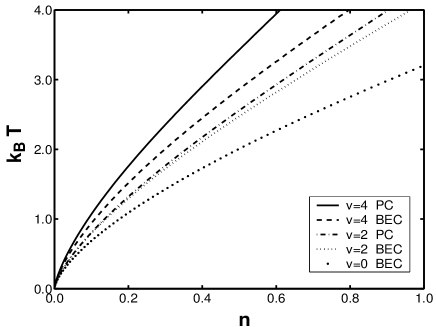
Figure 1: The transiton temperatures $T_{c}^{p}$ and $T_{c}^{b}$ versus density of particles $n$ for different interacting strength $v$. The solid and dash-dot lines indicate $T_{c}^{p}$, while the dashed and dotted lines indicate $T_{c}^{b}$. The asterisk line is $T_{c}^{b}$ for the ideal gas ($v=0$). $T_{c}^{p}>T_{c}^{b}$ for any positive $v$.

where $u^{2}={u^{\prime}}^{2}=(g+1)/2$, $v^{2}={v^{\prime}}^{2}=(g-1)/2$, $u^{\prime}v^{\prime}=-uv=g/f$, $g=f/\sqrt{f^{2}-4}$ and $f=\sqrt{3}{\bf k}^{2}/(v{\cal O})$, the Hamiltonian (44) can be diagonalized. The order parameter ${\cal O}$ and the chemical potential $\mu$ are determined by the following self-consistent equations

$$\frac{1}{v} = \frac{1}{4\pi^{2}}\int_{0}^{\epsilon_{F}}\frac{\sqrt{\epsilon}}{E}\coth\frac{\beta E}{2}d\epsilon,$$

$$n = \frac{1}{4\pi^{2}}\int_{0}^{\epsilon_{F}}\frac{3\sqrt{\epsilon}}{2}\left(\frac{\epsilon-\mu}{E}\coth\frac{\beta E}{2}-1\right)d\epsilon,$$ (46)

where $\epsilon_{F}$ is the energy cutoff or band width in an optical lattice, $E=\sqrt{(\epsilon-\mu)^{2}-4v^{2}{\cal O}^{2}/3}$, $n=\left\langle V^{-1}\sum_{s}\int a_{s}^{{\dagger}}({\bf r})a_{s}({\bf r})d{\bf r}\right\rangle_{T}$ is the density of particles, $\beta=1/T$. The critical temperature $T_{c}^{p}$ for pair condensation is determined by Eq. (46) with ${\cal O}|_{T\to T_{c}^{p}}=0$. Interestingly, besides the condensation of atom pairs, ordinary BEC also occurs at low temperature $T<T_{c}^{b}$ when $\mu=2v{\cal O}/\sqrt{3}$. The numerical solutions of $T_{c}^{b}$ and $T_{c}^{p}$ for $v=2,4$ are depicted in Fig. 1. It is shown that both $T_{c}^{b}$ and $T_{c}^{p}$ increase with increasing interacting strength $v$ and the density of particles $n$. Meanwhile, for a fixed $v$, $T_{c}^{p}$ is always larger than $T_{c}^{b}$. When $v\to 0$, $T_{c}^{p}\to T_{c}^{b}$. Below $T_{c}^{b}$, coexistence of pair condensation and BEC occurs. However, there is no BCS-BEC crossover which usually occurs in fermion gases.

VI Conclusion

In conclusion, we propose an exactly solvable model describing the low density limit of the spin-1 bosons in a 1D optical lattice. Based on the exact result, a mean-field approach for the corresponding 3D model is introduced. A new matter phase, i.e., the pair condensate and coexistence with ordinary BEC are predicted. We expect this new matter state could be realized in experiments.

- (1) T. -L. Ho, Phys. Rev. Lett. 81, 742 (1998).
- (2) T. Ohmi and K. Machida, J. Phys. Soc. Jpn. 67, 1822 (1998).
- (3) R. B. Diener and T. -L Ho, cond-mat/0608732.
- (4) C. J. Myatt, E. A. Burt, R. W. Ghrist, E. A. Cornell and C. E. Wieman, Phys. Rev. Lett. 78, 586 (1997).
- (5) D. M. Stamper-Kurn, M. R. Andrews, A. P. Chikkatur, S. Inouye, H. -J. Miesner, J. Stenger and W. Ketterle, Phys. Rev. Lett. 80, 2027 (1998).
- (6) J. Stenger, S. Inouye, D. M. Stamper-Kurn, H. -J. Miesner, A. P. Chikkatur and W. Ketterle, Nature 396, 345 (1998).
- (7) H. -J. Miesner, D. M. Stamper-Kurn, J. Stenger, S. Inouye, A. P. Chikkatur and W. Ketterle, Phys. Rev. Lett. 82, 2228 (1999).
- (8) E. Demler and F. Zhou, Phys. Rev. Lett. 88, 163001 (2002).
- (9) S. K. Yip, Phys. Rev. Lett. 90, 250402 (2003).
- (10) L. M. Duan. E. Demler and M. D. Lukin, Phys. Rev. Lett. 91, 090402 (2003).
- (11) A. A. Svidzinsky and S. T. Chui, Phys. Rev. A 68, 043612 (2003).
- (12) A. Imambekov, M. Lukin and E. Demler, Phys. Rev. Lett. 93, 120405 (2004).
- (13) M. Rizzi, D. Rossini, G. D. Chiara, S. Montangero and R. Fazio, Phys. Rev. Lett. 95, 240404 (2005).
- (14) M. P. A. Fisher, P. B. Weichman, G. Grinstein and D. S. Fisher, Phys. Rev. B 40, 546 (1989).
- (15) M. Greiner, O. Mandel, T. Esslinger, T. W. Hänsch and T. Bloch, Nature 415, 39 (2002).
- (16) A. Görlitz, J. M. Vogels, A. E. Leanhardt, C. Raman, T. L. Gustavson, J. R. Abo-Shaeer, A. P. Chikkatur, S. Gupta, S. Inouye, T. Rosenband and W. Ketterle, Phys. Rev. Lett. 87, 130402 (2001).
- (17) H. Moritz, T. Stöferle, M. Köhl and T. Esslinger, Phys. Rev. Lett. 91, 250402 (2003).
- (18) T. Stöferle, H. Moritz, C. Schori, M. Köhl and T. Esslinger, Phys. Rev. Lett. 92, 130403 (2004).
- (19) B. Paredes, A. Widera, V. Murg, O. Mandel, O. Fölling, T. Cirac, G. V. Shlyapnikov, T. W. Hänsch and I. Bloch, Nature 429, 277 (2004).
- (20) T. Kinoshita, T. Wenger and D. S. Weiss, Science 305, 1125 (2004).
- (21) B. L. Tolra, K. M. O’Hara, J. H. Huckans, W. D. Phillips, S. L. Rolston and J. V. Porto, Phys. Rev. Lett. 92, 190401 (2004).
- (22) J. W. Reijinders, F. J. M. van Lankvelt, K. Schoutens and N. Read, Phys. Rev. Lett. 89, 120401 (2002).
- (23) E. H. Lieb and W. Liniger, Phys. Rev. 130, 1605 (1963).
- (24) E. H. Lieb, Phys. Rev. 130, 1616 (1963).
- (25) J. N. Fuchs, A. Recati and W. Zwerger, Phys. Rev. Lett. 93, 090408 (2004).
- (26) E. H. Lieb and R. Seiringer, Phys. Rev. Lett. 91, 150401 (2003).
- (27) C. N. Yang, Phys. Rev. Lett. 19, 1312 (1967).
- (28) C. N. Yang, Phys. Rev. 168, 1920 (1968).
- (29) B. Sutherland, Phys. Rev. Lett. 20, 98 (1968).
- (30) L. A. Takhtajan, Phys. Lett. A 87, 479 (1982).
- (31) H. M. Babujian, Phys. Lett. A 90, 479 (1982).
- (32) K. -J. -B. Lee and P. Schlottmann, Phys. Rev. B 37, 379 (1988).
- (33) G. M. Zhang and L. Yu, cond-mat/0507158.
- (34) M. Takahashi, Thermodynamics of One-Dimensional Solvable Models (Cambridge University Press, Cambridge, 1999).