Scattering of elastic waves by elastic spheres in a NaCl-type phononic crystal

Abstract

Based on the formalism developed by Psarobas et al [Phys. Rev. B 62, 278(2000)], which using the multiple scattering theory to calculate properties of simple phononic crystals, we propose a very simple method to study the NaCl-type phononic crystal. The NaCl-type phononic crystal consists of two kinds of non-overlapping elastic spheres with different mass densities, $L\acute{a}me$ coefficients and radius following the same periodicity of the ions in the real NaCl crystal. We focus on the (001) surface, and view the crystal as a sequence of planes of spheres, each plane of spheres has identical 2D periodicity. We obtained the complex band structure of the infinite crystal associated with this plane, and also calculated the transmission, reflection and absorption coefficients for an elastic wave (longitudinal or transverse) incident, at any angle, on a slab of the crystal of finite thickness.

I Introduction

Recently, inspired by the remarkable properties of the photonic crystalsy , there has been increasing interest in the study of phononic crystalses ; khm ; mjt ; lzmz ; skek , which are constructed by composing identical particles (the inclusions) on host medium periodically. The acoustic behaviors in such materials are different from those in ordinary materials, such as the frequency band structure of classical waves and the propagation of elastic waves in the materials. Various applications are also proposed, for example, acoustic lenscssm , waveguidesmi and negative refraction materialssss . The behaviors of the new materials are related to their band structures so that the calculation of the acoustic wave spectrum, or band structure is the key point in the studies of phononic crystals.

There are several techniques for the calculation of frequency band structures, the plane-wave approach is the simplest though the convergence is slowes ; khm ; mjt , the multiple-scattering theory (MST) or KKR (Korringa, Kohn, and Rostoker) approach are widely used with better convergencepsm ; lcsgp ; sspm , and the finite difference time domain (FDTD) method is a new and promising methodt . When the inclusions of phononic crystals are spheres in 3-dimensional case or cylinders in 2-dimensional case, layer MST is a very effective calculation technique not only for the evaluation of band structures, but also for the calculation of the transmission, reflection and absorption coefficients of a slab of the crystal of finite thickness. Based on the layer MST approach, Psarobas et al psm ; sspm have developed a formalism for calculating the frequency band structure of phononic crystals and the corresponding scattering properties. In their algorithm and the related program package, they consider only the 3-dimensional phononic crystals formed by one inclusion per unit cell, so the phononic crystals are the so called “simple” crystals. In addition to band structure, their program package can also deal with scattering problems with a slab of crystals of finite thickness, if all successional scattering planes are 2-dimensional “simple” lattices.

However, it is desirable to have a technique to deal with “complex” phononic crystals (i.e. crystals have more than one type of inclusion per unit cell). The crystals with “complex” structures may offer us different band gaps and new properties which are not existed in “simple” crystals. By generalizing the simple lattice layer MST method, we propose here a simple technique to deal with NaCl-type “complex” phononic crystals by means of MST. Calculation of the band structures is made and compared to the “simple” case. A general method to work with “complex” phononic crystals, which are similar to those in low energy electron diffraction of “complex” crystalsp , is also discussed in Appendix A. Our method is based on MST and different from the plane-wave approach suggested by Zhang et alzllw , so it is more efficient in dealing with spherical inclusion, and the case of fluid-solid composites. In addition, one may notice that the NaCl-type crystal can also be seen as a succession of two nonoverlapping planes of different spheres in the (111) direction and considered as a heterostructure sspm or as a case of a super cell with planar defects psm2 , so the complex band structure could be extracted from their program. Actually, Liu et allcs have also used their bulk KKR method to calculate the full band structure of some complex phononic crystals with HCP and Diamond structure. However, the layer KKR method here we used is necessary, since it can also be used to calculate the transmission, reflection and absorption coefficients for an elastic wave incident on a slab of NaCl-type “complex” crystal. Recently, it has also been applied to a chiral structure, which is regarded as a more complex heterostructure, many interesting results was found cc . The programm package developed by Sainidou et alsspm is a stable and efficient package in treating the simple phononic crystals, we have used the package extensively in our “complex” phononic crystal calculation.

The paper is organized as follows. In section II, we present a simple method to evaluate the scattering properties of a slab consisting a number of layers, which could contain two kinds of spheres with specific 2D periodic structure. In section III, we demonstrate the applicability of our method with some numerical results and discussions. Finally, the conclusions of the paper are given in Sec. IV.

II Theory

In this section, we briefly review the theory of layer MST used in the calculation of band structures of phononic crystals with the NaCl-type structure. Firstly, we consider a “complex” 2D crystal in $xy$-plane at $z=0$. There are two kinds of spheres in the 2D crystal. The first is denoted as type A, located on the sites of a 2D lattice specified by

$$\mathbf{R}_{n}=n_{1}\mathbf{a}_{1}+n_{2}\mathbf{a}_{2},$$ (1)

where $\mathbf{a}_{1}$,$\mathbf{a}_{2}$ are the primitive vectors of a 2D lattice in the $xy$-plane, and $n_{1},n_{2}=0,\pm 1,\pm 2,\pm 3,...$. The second kind of spheres is denoted as type B, located at

$$\mathbf{R}_{n}^{b}=\overrightarrow{ab}+\mathbf{R}_{n}=\overrightarrow{ab}+n_{1}\mathbf{a}_{1}+n_{2}\mathbf{a}_{2},$$ (2)

where $\overrightarrow{ab}=(\mathbf{a}_{1}+\mathbf{a}_{2})/2$ for NaCl-type phononic crystal. In this case, there are two types of inclusion per unit cell, and the corresponding 2D reciprocal lattice is

$$\mathbf{g}=m_{1}\mathbf{b}_{1}+m_{2}\mathbf{b}_{2},$$ (3)

where $m_{1},m_{2}=0,\pm 1,\pm 2,\pm 3,...$ and vectors $\mathbf{b}_{1}$, $\mathbf{b}_{2}$ are defined by

$$\mathbf{b}_{i}\cdot\mathbf{a}_{j}=2\pi\delta_{ij},\quad\quad i,j=1,2.$$ (4)

Now we consider that a plane wave, either longitudinal or transverse, is incident onto such a plane of spheres of type A and B. The displacement vector of the incident wave has the formpsm ,

$$\mathbf{u}_{in}^{s^{\prime}}(\mathbf{r})=\sum_{i^{\prime}}[u_{in}]_{\mathbf{g}^{\prime}i^{\prime}}^{s^{\prime}}\exp(i\mathbf{K}_{\mathbf{g}^{\prime}\nu^{\prime}}^{s^{\prime}}\cdot\mathbf{r})\hat{\mathbf{e}}_{i^{\prime}},$$ (5)

where $s^{\prime}=+(-)$ represents that a wave is incident onto the plane from the left(right), $\nu^{\prime}$ denotes the polarization of the incident wave: $q_{\nu^{\prime}}=q_{l}=\omega/c_{l}$ for a longitudinal wave and $q_{\nu^{\prime}}=q_{t}=\omega/c_{t}$ for a transverse one. Because of the 2D periodicity in the plane of spheres, wavevector can be rewritten as

$$\mathbf{K}_{\mathbf{g}^{\prime}\nu^{\prime}}^{\pm}\equiv\mathbf{k}_{||}+\mathbf{g}^{\prime}\pm[q_{\nu^{\prime}}^{2}-(\mathbf{k}_{||}+\mathbf{g}^{\prime})^{2}]^{1/2}\hat{\mathbf{e}}_{z},$$ (6)

where $\hat{\mathbf{e}}_{z}$ is the unit vector along the $z$ axis, $\mathbf{k}_{||}$ is the reduced wave vector lying in the surface Brillouin zone (SBZ) of the given lattice, and $\mathbf{g}^{\prime}$ is one of the reciprocal lattice vectors in Eq.(3).

In order to avoid the cumbersome formulas in the representation of the displacement field, we use the same complete set of spherical-wave solutions as recommended by Sainidou et alsspm ,

$$\begin{array}[]{ll}\mathbf{J}_{Llm}(\mathbf{r})=\frac{1}{q_{l}}\nabla[j_{l}(q_{l}r)Y_{l}^{m}(\hat{\mathbf{r}})],&\quad\mathbf{H}_{Llm}(\mathbf{r})=\frac{1}{q_{l}}\nabla[h_{l}^{+}(q_{l}r)Y_{l}^{m}(\hat{\mathbf{r}})],\\ \mathbf{J}_{Mlm}(\mathbf{r})=j_{l}(q_{t}r)\mathbf{X}_{lm}(\hat{\mathbf{r}}),&\quad\mathbf{H}_{Mlm}(\mathbf{r})=h_{l}^{+}(q_{t}r)\mathbf{X}_{lm}(\hat{\mathbf{r}}),\\ \mathbf{J}_{Nlm}(\mathbf{r})=\frac{i}{q_{t}}\nabla\times j_{l}(q_{t}r)\mathbf{X}_{lm}(\hat{\mathbf{r}}),&\quad\mathbf{H}_{Nlm}(\mathbf{r})=\frac{i}{q_{t}}\nabla\times h_{l}^{+}(q_{t}r)\mathbf{X}_{lm}(\hat{\mathbf{r}}),\end{array}$$ (7)

here $j_{l}$ and $h^{+}_{l}$ are the spherical Bessel and Hankel functions, $Y_{l}^{m}$ and $\mathbf{X}_{lm}$ are the usual and vector spherical harmonics, respectively.

The scattered waves by all spheres in the plane can be separated into two parts. One is the contributions from spheres of type A, $\mathbf{u}_{sc}^{As}(\mathbf{r})$, and the other is those from spheres of type B, $\mathbf{u}_{sc}^{Bs}(\mathbf{r}^{\prime})$, here $\mathbf{r}=\mathbf{r}^{\prime}+\overrightarrow{ab}$. Let $a_{n,lm}^{+P}(P=L,M,N)$ be the scatter wave coefficients of sphere A at the site $R_{n}$. According to the Bloch theorem, we have

$$\mathbf{u}_{sc}^{As}(\mathbf{r})=\sum_{n,Plm}a_{n,lm}^{+P}\mathbf{H}_{Plm}(\mathbf{r}_{n})=\sum_{Plm}a_{lm}^{+P}\sum_{\mathbf{R}_{n}}\exp(i\mathbf{k}_{||}\cdot\mathbf{R}_{n})\mathbf{H}_{Plm}(\mathbf{r}-\mathbf{R}_{n}).$$ (8)

where $a_{lm}^{+P}(P=L,M,N)$ are the scatter wave coefficients of sphere A at the origin. In the domain close to surface of sphere of type B, it is always satisfied that $|\mathbf{r}^{\prime}|<|\mathbf{R}_{n}-\overrightarrow{ab}|$ since all spheres are not overlapped. So that the $\mathbf{u}_{sc}^{As}(\mathbf{r})$ can be expanded into spherical waves about the sphere of type B, which is located at $\overrightarrow{ab}$, as follows

$$\mathbf{u}_{sc}^{As}(\mathbf{r})=\exp(i\mathbf{K}_{\mathbf{g}^{\prime}\nu^{\prime}}^{s^{\prime}}\cdot\overrightarrow{ab})\sum_{Plm}d_{lm}^{{}^{\prime}P}\mathbf{J}_{Plm}(\mathbf{r}^{\prime}).$$ (9)

Likewise, we have

$$\begin{array}[]{rcl}\mathbf{u}_{sc}^{Bs}(\mathbf{r}^{\prime})&=&\displaystyle\exp(i\mathbf{K}_{\mathbf{g}^{\prime}\nu^{\prime}}^{s^{\prime}}\cdot\overrightarrow{ab})\sum_{n,Plm}b_{n,lm}^{+P}\mathbf{H}_{Plm}(\mathbf{r}_{n}^{\prime})\\ &=&\displaystyle\exp(i\mathbf{K}_{\mathbf{g}^{\prime}\nu^{\prime}}^{s^{\prime}}\cdot\overrightarrow{ab})\sum_{Plm}b_{lm}^{+P}\sum_{\mathbf{R}_{n}}\exp(i\mathbf{k}_{||}\cdot\mathbf{R}_{n})\mathbf{H}_{Plm}(\mathbf{r}^{\prime}-\mathbf{R}_{n}),\end{array}$$ (10)

it can also be expanded as follows

$$\mathbf{u}_{sc}^{Bs}(\mathbf{r}^{\prime})=\sum_{Plm}c_{lm}^{{}^{\prime}P}\mathbf{J}_{Plm}(\mathbf{r}).$$ (11)

In addition, the external incident wave is

$$\mathbf{u}_{in}(\mathbf{r})=\sum_{Plm}a_{lm}^{0P}\mathbf{J}_{Plm}(\mathbf{r})=\exp(i\mathbf{K}_{\mathbf{g}^{\prime}\nu^{\prime}}^{s^{\prime}}\cdot\overrightarrow{ab})\sum_{Plm}a_{lm}^{0P}\mathbf{J}_{Plm}(\mathbf{r}^{\prime}).$$ (12)

Moreover, if we remove the term corresponding to sphere located at $\mathbf{R}_{n}=0$ in Eq. (8), the terms left are just the scattering waves come from all spheres of type A except for itself. We denote it by $\mathbf{u}_{sc}^{As\prime}(\mathbf{r})$, and expand it into spherical waves about the origin

$$\mathbf{u}_{sc}^{As\prime}(\mathbf{r})=\sum_{Plm}a_{lm}^{{}^{\prime}P}\mathbf{J}_{Plm}(\mathbf{r}).$$ (13)

In the same way, after removing the term corresponding to $\mathbf{R}_{n}=0$ in Eq. (10), we have

$$\mathbf{u}_{sc}^{Bs\prime}(\mathbf{r}^{\prime})=\exp(i\mathbf{K}_{\mathbf{g}^{\prime}\nu^{\prime}}^{s^{\prime}}\cdot\overrightarrow{ab})\sum_{Plm}b_{lm}^{{}^{\prime}P}\mathbf{J}_{Plm}(\mathbf{r}^{\prime}).$$ (14)

It means the scattering waves come from all spheres of type B except for the one located at $\overrightarrow{ab}$. It can be shown from direct calculation (see Appendix A for the details) that

$$\begin{array}[]{cc}\displaystyle a_{lm}^{{}^{\prime}P}=\sum_{P^{\prime}l^{\prime}m^{\prime}}\Omega_{lm;l^{\prime}m^{\prime}}^{PP^{\prime}}a_{l^{\prime}m^{\prime}}^{+P^{\prime}},&\quad\displaystyle b_{lm}^{{}^{\prime}P}=\sum_{P^{\prime}l^{\prime}m^{\prime}}\Omega_{lm;l^{\prime}m^{\prime}}^{PP^{\prime}}b_{l^{\prime}m^{\prime}}^{+P^{\prime}},\\ \displaystyle c_{lm}^{{}^{\prime}P}=\sum_{P^{\prime}l^{\prime}m^{\prime}}\Xi_{lm;l^{\prime}m^{\prime}}^{PP^{\prime}}b_{l^{\prime}m^{\prime}}^{+P^{\prime}},&\quad\displaystyle d_{lm}^{{}^{\prime}P}=\sum_{P^{\prime}l^{\prime}m^{\prime}}\Xi_{lm;l^{\prime}m^{\prime}}^{PP^{\prime}}a_{l^{\prime}m^{\prime}}^{+P^{\prime}}.\end{array}$$ (15)

According to MST, the wave incident on the sphere of type A located at the origin consists of three parts, the first party is the externally incident wave, the second part is the sum of all the waves scattered by spheres of type A except for itself, and the third part is the sum of all the waves scattered by spheres of type B. The coefficients of the incident wave and scattering wave is related to each other by the Mie matrix, so we have the following relationship

$$a_{lm}^{+P}=\sum_{P^{\prime}l^{\prime}m^{\prime}}T_{a;lm;l^{\prime}m^{\prime}}^{PP^{\prime}}(a_{l^{\prime}m^{\prime}}^{0P^{\prime}}+a_{l^{\prime}m^{\prime}}^{{}^{\prime}P^{\prime}}+c_{l^{\prime}m^{\prime}}^{{}^{\prime}P^{\prime}}).$$ (16)

Likewise, the wave incident on the sphere B located at $\overrightarrow{ab}$ also consists of three parts, the externally incident wave, the sum of all the waves scattered by spheres of type B except for itself, and the sum of all the waves scattered by spheres of type A, so we have

$$b_{lm}^{+P}=\sum_{P^{\prime}l^{\prime}m^{\prime}}T_{b;lm;l^{\prime}m^{\prime}}^{PP^{\prime}}\left(a_{l^{\prime}m^{\prime}}^{0P^{\prime}}+b_{l^{\prime}m^{\prime}}^{{}^{\prime}P^{\prime}}+d_{l^{\prime}m^{\prime}}^{{}^{\prime}P^{\prime}}\right).$$ (17)

Combining Eqs. (15), (16) and (17), we obtain

$$\begin{array}[]{l}\displaystyle\sum_{P^{\prime}l^{\prime}m^{\prime}}\left[\delta_{PP^{\prime}}\delta_{ll^{\prime}}\delta_{mm^{\prime}}-\sum_{P^{\prime\prime}l^{\prime\prime}m^{\prime\prime}}T_{a;lm;l^{\prime\prime}m^{\prime\prime}}^{PP^{\prime\prime}}\Omega_{l^{\prime\prime}m^{\prime\prime};l^{\prime}m^{\prime}}^{P^{\prime\prime}P^{\prime}}\right]a_{l^{\prime}m^{\prime}}^{+P^{\prime}}\\ \qquad\qquad\qquad\quad\displaystyle+\sum_{P^{\prime}l^{\prime}m^{\prime}}\left[-\sum_{P^{\prime\prime}l^{\prime\prime}m^{\prime\prime}}T_{a;lm;l^{\prime\prime}m^{\prime\prime}}^{PP^{\prime\prime}}\Xi_{l^{\prime\prime}m^{\prime\prime};l^{\prime}m^{\prime}}^{P^{\prime\prime}P^{\prime}}\right]b_{l^{\prime}m^{\prime}}^{+P^{\prime}}=\sum_{P^{\prime}l^{\prime}m^{\prime}}T_{a;lm;l^{\prime}m^{\prime}}^{PP^{\prime}}a_{l^{\prime}m^{\prime}}^{0P^{\prime}},\\ \displaystyle\sum_{P^{\prime}l^{\prime}m^{\prime}}\left[-\sum_{P^{\prime\prime}l^{\prime\prime}m^{\prime\prime}}T_{b;lm;l^{\prime\prime}m^{\prime\prime}}^{PP^{\prime\prime}}\Xi_{l^{\prime\prime}m^{\prime\prime};l^{\prime}m^{\prime}}^{P^{\prime\prime}P^{\prime}}\right]a_{l^{\prime}m^{\prime}}^{+P^{\prime}}\\ \quad\quad\displaystyle+\sum_{P^{\prime}l^{\prime}m^{\prime}}\left[\delta_{PP^{\prime}}\delta_{ll^{\prime}}\delta_{mm^{\prime}}-\sum_{P^{\prime\prime}l^{\prime\prime}m^{\prime\prime}}T_{b;lm;l^{\prime\prime}m^{\prime\prime}}^{PP^{\prime\prime}}\Omega_{l^{\prime\prime}m^{\prime\prime};l^{\prime}m^{\prime}}^{P^{\prime\prime}P^{\prime}}\right]b_{l^{\prime}m^{\prime}}^{+P^{\prime}}=\sum_{P^{\prime}l^{\prime}m^{\prime}}T_{b;lm;l^{\prime}m^{\prime}}^{PP^{\prime}}a_{l^{\prime}m^{\prime}}^{0P^{\prime}}.\end{array}$$ (18)

When the coefficients $a_{lm}^{0P}$ of the incident wave are given, equations (18) determine the scattering coefficients $a_{lm}^{+P}$ and $b_{lm}^{+P}$ of spheres of type A and B. Consequently, the waves scattered from the plane of spheres of type A and B are also obtained in terms of Eqs. (8) and (10), respectively.

We write the coefficients $a_{lm}^{0P}$ in the form of

$$a_{lm}^{0P}=\sum_{i^{\prime}}A_{lm;i^{\prime}}^{0P}(\mathbf{K}_{\mathbf{g}^{\prime}\nu^{\prime}}^{s^{\prime}})[u_{in}]_{\mathbf{g}^{\prime}i^{\prime}}^{s^{\prime}}$$ (19)

based on Eq. (5), where coefficients $A_{lm}^{0P}$ are given in Psarobas et alpsm (Eqs. (3.4), (3.7) and (3.8)). Because of the linearity of Eqs. (18), the coefficients $a_{lm}^{+P}$ and $b_{lm}^{+P}$ can also be written as follows

$$a_{lm}^{+P}=\sum_{i^{\prime}}A_{lm;i^{\prime}}^{+P}(\mathbf{K}_{\mathbf{g}^{\prime}\nu^{\prime}}^{s^{\prime}})[u_{in}]_{\mathbf{g}^{\prime}i^{\prime}}^{s^{\prime}},$$ (20)

$$b_{lm}^{+P}=\sum_{i^{\prime}}B_{lm;i^{\prime}}^{+P}(\mathbf{K}_{\mathbf{g}^{\prime}\nu^{\prime}}^{s^{\prime}})[u_{in}]_{\mathbf{g}^{\prime}i^{\prime}}^{s^{\prime}},$$ (21)

so that the Eqs. (18) are reduced to

$$\begin{array}[]{l}\displaystyle\sum_{P^{\prime}l^{\prime}m^{\prime}}\left[\delta_{PP^{\prime}}\delta_{ll^{\prime}}\delta_{mm^{\prime}}-\sum_{P^{\prime\prime}l^{\prime\prime}m^{\prime\prime}}T_{a;lm;l^{\prime\prime}m^{\prime\prime}}^{PP^{\prime\prime}}\Omega_{l^{\prime\prime}m^{\prime\prime};l^{\prime}m^{\prime}}^{P^{\prime\prime}P^{\prime}}\right]A_{l^{\prime}m^{\prime};i^{\prime}}^{+P^{\prime}}(\mathbf{K}_{\mathbf{g}^{\prime}\nu^{\prime}}^{s^{\prime}})\\ \displaystyle\quad+\sum_{P^{\prime}l^{\prime}m^{\prime}}\left[-\sum_{P^{\prime\prime}l^{\prime\prime}m^{\prime\prime}}T_{a;lm;l^{\prime\prime}m^{\prime\prime}}^{PP^{\prime\prime}}\Xi_{l^{\prime\prime}m^{\prime\prime};l^{\prime}m^{\prime}}^{P^{\prime\prime}P^{\prime}}\right]B_{l^{\prime}m^{\prime};i^{\prime}}^{+P^{\prime}}(\mathbf{K}_{\mathbf{g}^{\prime}\nu^{\prime}}^{s^{\prime}})=\sum_{P^{\prime}l^{\prime}m^{\prime}}T_{a;lm;l^{\prime}m^{\prime}}^{PP^{\prime}}A_{l^{\prime}m^{\prime};i^{\prime}}^{0P^{\prime}}(\mathbf{K}_{\mathbf{g}^{\prime}\nu^{\prime}}^{s^{\prime}}),\\ \displaystyle\sum_{P^{\prime}l^{\prime}m^{\prime}}\left[-\sum_{P^{\prime\prime}l^{\prime\prime}m^{\prime\prime}}T_{b;lm;l^{\prime\prime}m^{\prime\prime}}^{PP^{\prime\prime}}\Xi_{l^{\prime\prime}m^{\prime\prime};l^{\prime}m^{\prime}}^{P^{\prime\prime}P^{\prime}}\right]A_{l^{\prime}m^{\prime};i^{\prime}}^{+P^{\prime}}(\mathbf{K}_{\mathbf{g}^{\prime}\nu^{\prime}}^{s^{\prime}})\\ \displaystyle\quad+\sum_{P^{\prime}l^{\prime}m^{\prime}}\left[\delta_{PP^{\prime}}\delta_{ll^{\prime}}\delta_{mm^{\prime}}-\sum_{P^{\prime\prime}l^{\prime\prime}m^{\prime\prime}}T_{b;lm;l^{\prime\prime}m^{\prime\prime}}^{PP^{\prime\prime}}\Omega_{l^{\prime\prime}m^{\prime\prime};l^{\prime}m^{\prime}}^{P^{\prime\prime}P^{\prime}}\right]B_{l^{\prime}m^{\prime};i^{\prime}}^{+P^{\prime}}(\mathbf{K}_{\mathbf{g}^{\prime}\nu^{\prime}}^{s^{\prime}})\\ \displaystyle\quad=\sum_{P^{\prime}l^{\prime}m^{\prime}}T_{b;lm;l^{\prime}m^{\prime}}^{PP^{\prime}}A_{l^{\prime}m^{\prime};i^{\prime}}^{0P^{\prime}}(\mathbf{K}_{\mathbf{g}^{\prime}\nu^{\prime}}^{s^{\prime}}).\end{array}$$ (22)

Now, the scattered waves given by Eqs. (8) and (10) are expressed as sum of plane waves as follows (see Appendix B)

$$\begin{array}[]{rcl}\mathbf{u}_{sc}^{As}(\mathbf{r})&=&\displaystyle\sum_{\mathbf{g}i}[u_{sc}^{A}]_{\mathbf{g}i}^{s}\exp(i\mathbf{K}_{\mathbf{g}\nu}^{s}\cdot\mathbf{r})\hat{\mathbf{e}}_{i},\\ \mathbf{u}_{sc}^{Bs}(\mathbf{r}^{\prime})&=&\displaystyle\exp(i\mathbf{K}_{\mathbf{g}^{\prime}\nu^{\prime}}^{s^{\prime}}\cdot\overrightarrow{ab})\sum_{\mathbf{g}i}[u_{sc}^{\prime B}]_{\mathbf{g}i}^{s}\exp(i\mathbf{K}_{\mathbf{g}\nu}^{s}\cdot\mathbf{r}^{\prime})\hat{\mathbf{e}}_{i}=\sum_{\mathbf{g}i}[u_{sc}^{B}]_{\mathbf{g}i}^{s}\exp(i\mathbf{K}_{\mathbf{g}\nu}^{s}\cdot\mathbf{r})\hat{\mathbf{e}}_{i}.\end{array}$$ (23)

Here $u_{sc}^{\prime B}$ is obtained in coordinates ${\bf r}^{\prime}$, it is obviously that its expression is similar to $u_{sc}^{A}$. The total scattered wave then becomes

$$\mathbf{u}_{sc}^{s}(\mathbf{r})=\sum_{\mathbf{g}i}([u_{sc}^{A}]_{\mathbf{g}i}^{s}+[u_{sc}^{B}]_{\mathbf{g}i}^{s})\exp(i\mathbf{K}_{\mathbf{g}\nu}^{s}\cdot\mathbf{r})\hat{\mathbf{e}}_{i},$$ (24)

where $[u_{sc}^{A}]_{\mathbf{g}i}^{s}$ and $[u_{sc}^{B}]_{\mathbf{g}i}^{s}$ are given by

$$[u_{sc}^{A}]_{\mathbf{g}i}^{s}=\sum_{i^{\prime}}\sum_{Plm}\Delta_{lm;i}^{P}(\mathbf{K}_{\mathbf{g}\nu}^{s})A_{lm;i^{\prime}}^{+P}(\mathbf{K}_{\mathbf{g}^{\prime}\nu^{\prime}}^{s^{\prime}})[u_{in}]_{\mathbf{g}^{\prime}i^{\prime}}^{s^{\prime}},$$ (25)

$$[u_{sc}^{B}]_{\mathbf{g}i}^{s}=\sum_{i^{\prime}}\sum_{Plm}\Delta_{lm;i}^{P}(\mathbf{K}_{\mathbf{g}\nu}^{s})B_{lm;i^{\prime}}^{+P}(\mathbf{K}_{\mathbf{g}^{\prime}\nu^{\prime}}^{s^{\prime}})[u_{in}]_{\mathbf{g}^{\prime}i^{\prime}}^{s^{\prime}}\exp{(i(\mathbf{K}_{\mathbf{g}^{\prime}\nu^{\prime}}^{s^{\prime}}-\mathbf{K}_{\mathbf{g}\nu}^{s})\cdot\overrightarrow{ab})}.$$ (26)

The derivation is given in Appendix B.

With these results, we get this 2D “complex” crystal’s $\mathbf{M}$-matrix elements

$$M_{\mathbf{g}i;\mathbf{g}^{\prime}i^{\prime}}^{ss^{\prime}}=\delta_{ss^{\prime}}\delta_{\mathbf{g}\mathbf{g}^{\prime}}\delta_{ii^{\prime}}+\sum_{Plm}\Delta_{lm;i}^{P}(\mathbf{K}_{\mathbf{g}\nu}^{s})[A_{lm;i^{\prime}}^{+P}(\mathbf{K}_{\mathbf{g}^{\prime}\nu^{\prime}}^{s^{\prime}})+B_{lm;i^{\prime}}^{+P}(\mathbf{K}_{\mathbf{g}^{\prime}\nu^{\prime}}^{s^{\prime}})\exp{(i(\mathbf{K}_{\mathbf{g}^{\prime}\nu^{\prime}}^{s^{\prime}}-\mathbf{K}_{\mathbf{g}\nu}^{s})\cdot\overrightarrow{ab})}].$$ (27)

Using the algorithm recommended by Psarobas et alpsm ; sspm , as soon as the $\mathbf{M}$-matrix is given, both the frequency band structure of an infinite crystal and acoustic properties of a slab of this crystal can be calculated in the same way. Here we only write down the $\mathbf{Q}$-matrix elements

$$\begin{array}[]{rcl}Q_{\mathbf{g}i;\mathbf{g}^{\prime}i^{\prime}}^{I}&=&M_{\mathbf{g}i;\mathbf{g}^{\prime}i^{\prime}}^{++}\exp\left[i(\mathbf{K}_{\mathbf{g}\nu}^{+}\cdot\mathbf{d}_{r}+\mathbf{K}_{\mathbf{g}^{\prime}\nu^{\prime}}^{+}\cdot\mathbf{d}_{l})\right],\\ Q_{\mathbf{g}i;\mathbf{g}^{\prime}i^{\prime}}^{II}&=&M_{\mathbf{g}i;\mathbf{g}^{\prime}i^{\prime}}^{+-}\exp\left[i(\mathbf{K}_{\mathbf{g}\nu}^{+}\cdot\mathbf{d}_{r}-\mathbf{K}_{\mathbf{g}^{\prime}\nu^{\prime}}^{-}\cdot\mathbf{d}_{r})\right],\\ Q_{\mathbf{g}i;\mathbf{g}^{\prime}i^{\prime}}^{III}&=&M_{\mathbf{g}i;\mathbf{g}^{\prime}i^{\prime}}^{-+}\exp\left[-i(\mathbf{K}_{\mathbf{g}\nu}^{-}\cdot\mathbf{d}_{l}-\mathbf{K}_{\mathbf{g}^{\prime}\nu^{\prime}}^{+}\cdot\mathbf{d}_{l})\right],\\ Q_{\mathbf{g}i;\mathbf{g}^{\prime}i^{\prime}}^{IV}&=&M_{\mathbf{g}i;\mathbf{g}^{\prime}i^{\prime}}^{--}\exp\left[-i(\mathbf{K}_{\mathbf{g}\nu}^{-}\cdot\mathbf{d}_{l}+\mathbf{K}_{\mathbf{g}^{\prime}\nu^{\prime}}^{-}\cdot\mathbf{d}_{r})\right].\end{array}$$ (28)

III Numerical results and discussion

We demonstrate the applicability of our method by applying it to two specific examples. Firstly, we illustrate the 2D periodic structure of NaCl-type phononic crystal in figure 1, here the nearest distance between the same spheres is defined as lattice constant $a_{0}$, so that $\mathbf{a}_{1}=a_{0}(1,0,0)$ and $\mathbf{a}_{2}=a_{0}(0,1,0)$ in Eqs. (1) and (2). Then we choose $\mathbf{d}_{l}=\mathbf{d}_{r}=a_{0}(0.25,0.25,\sqrt{2}/4)$ in Eq. (28)sspm , and obtain a slab of NaCl-type phononic crystal of finite thickness associated with the (001) surface. We take $a_{0}=1cm$ in the calculation.

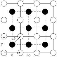
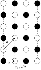
Figure 1: The 2D structure of each layer of (001) plane is given in the left graph, the lattice constant $a_{0}$ is the nearest distance between the same spheres, the distance between two neighbor layers is $a_{0}/\sqrt{2}$ for NaCl-type phononic crystal (the right graph is the section perpendicular to the layer plane).

In figure 2, we show the transmittance curves of a slab of 8 layers parallel to the (001) surface of NaCl-type phononic crystal at normal incident for longitudinal wave (a) and transverse wave (b). The materials are: sphere of type A is lead sphere of radius $S=0.25cm$, sphere of type B is lead sphere of radius $S=0.10cm$, the host matrix is epoxy. The relevant parameters are, for lead: $\rho=11.6\times 10^{3}kg/m^{3}$, $c_{l}=2490m/s$, $c_{t}=1130m/s$, and for epoxy: $\rho=1.18\times 10^{3}kg/m^{3}$, $c_{l}=2540m/s$, $c_{t}=1160m/s$. Figure 3 shows the corresponding complex band structure of the infinite NaCl-type phononic crystal associated with the (001) surface. All the units are following the suggestion given by Sainidou et al sspm , where $c_{0}=2540m/s$.

Figure 2: The transmittance curves of a slab of 8 layers parallel to (001) surface of NaCl-type phononic crystal at normal incident for longitudinal wave (a the upper graph) and transverse wave (b the lower graph).

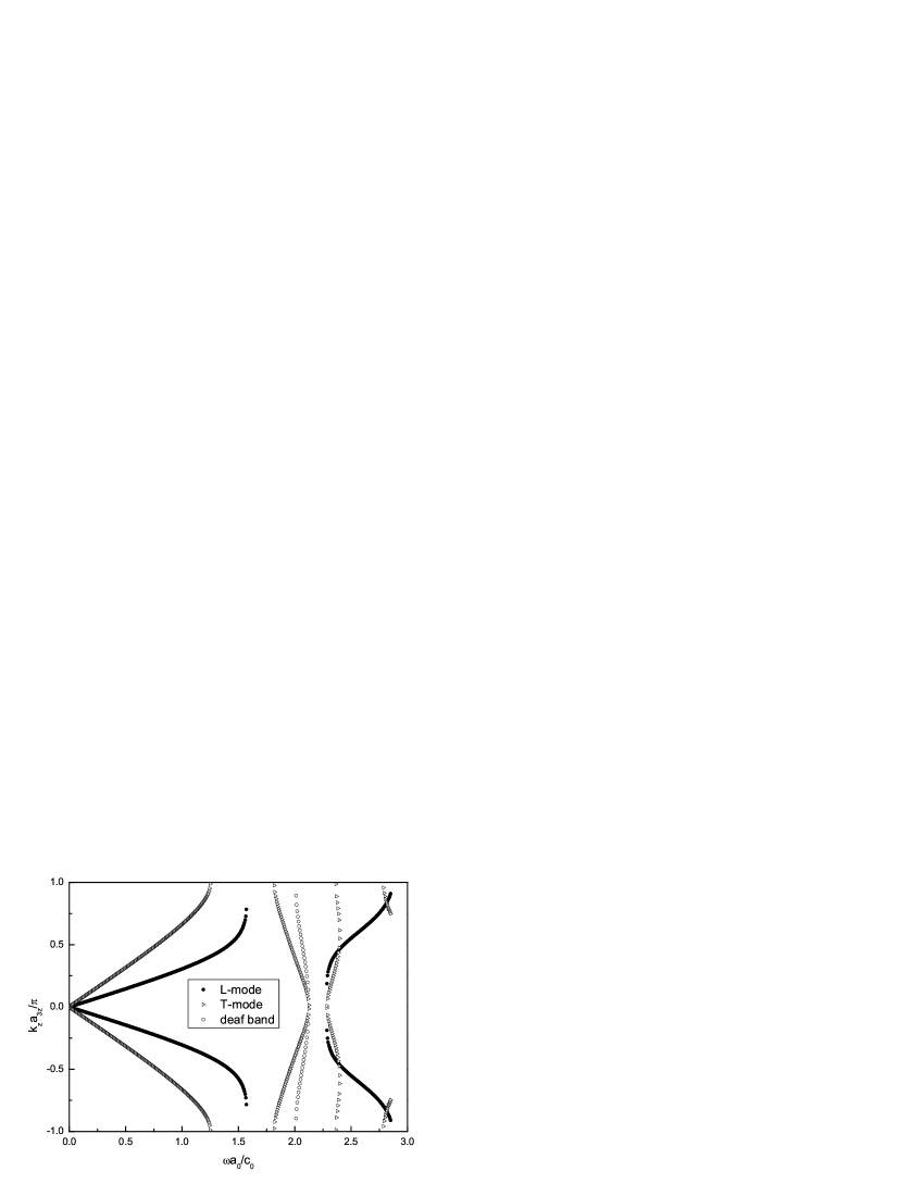
Figure 3: The phononic band structure at the center of the SBZ of a (001) surface of NaCl-type phononic crystal corresponding to Fig.2. The filled circles represent the longitudinal mode, the open triangles represent the transverse modes and the open circles represent the deaf band, respectively.

Comparing the results in figure 2 and figure 3, we see that there is a frequency band gap approximate between 1.6 to 2.25 for the longitudinal wave, and also several band gaps for the transverse wave. It should be noted that the width of the gaps and the positions have all changed from those of the traditional “simple” phononic crystal, so that a lot of work has to be done for searching some new properties of this kind of phononic crystals.

In figure 4 we show the reflectance curve of a slab of layers parallel to the same surface at normal incident for longitudinal wave. The materials are taken as follows: sphere of type A is lead sphere of radius $S=0.20cm$ coated with a $0.5mm$ layer of silicone rubber, sphere of type B is silica sphere of radius $S=0.10cm$ coated with a $1.5mm$ layer of silicone rubber, the host matrix is epoxy. The relevant parameters are, for lead: $\rho=11.6\times 10^{3}kg/m^{3}$, $c_{l}=2490m/s$, $c_{t}=1130m/s$, for silicone rubber: $\rho=1.3\times 10^{3}kg/m^{3}$, $c_{l}=22.87m/s$, $c_{t}=5.55m/s$, for silica: $\rho=2.2\times 10^{3}kg/m^{3}$, $c_{l}=5970m/s$, $c_{t}=3760m/s$, and for epoxy: $\rho=1.18\times 10^{3}kg/m^{3}$, $c_{l}=2540m/s$, $c_{t}=1160m/s$. We take such materials that the spheres of type A and B have different local resonance frequencies, which can be estimated in the approach of Liu et allzmz .

When the NaCl-type phononic crystal is consisted of two kinds of local resonance materials, our results show that both of local the resonance frequency (see the peaks with amplitude close to 1 that represents total reflectance) are still keep unchanged, which means that this kind of hybrid does not change the property of intrinsic local resonance. In addition, as the number of the layers increased, the band gap is broadened indicate by the broader peak. We also see that there is a small wiggle near $0.11$. In fact, when we scan the frequency in more refined steps, we found that there is a very sharp resonance located at there. The corresponding frequency band structure is shown in figure 5.

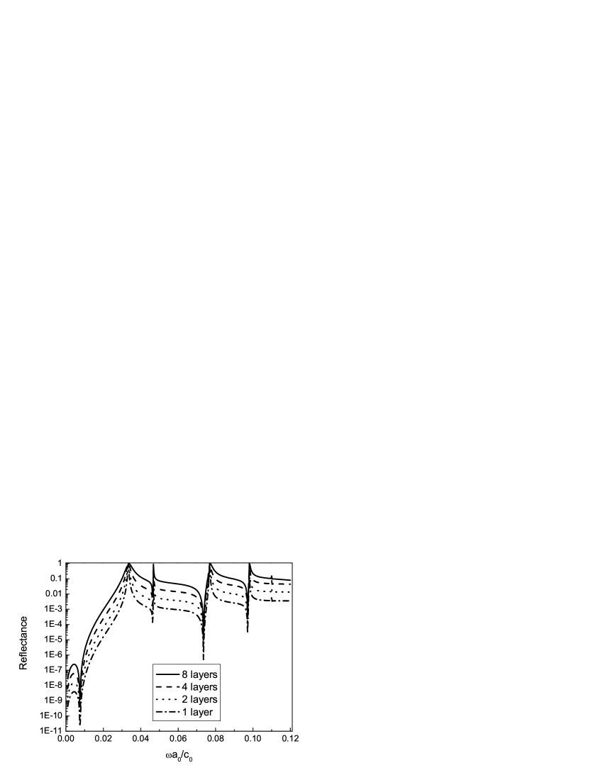
Figure 4: The reflectance curves of a slab of different layers parallel to (001) surface of NaCl-type phononic crystal at normal incident for longitudinal wave for local resonance materials. The solid, dash, dot and dot-dash line are for 8, 4, 2 and single layer, respectively.

Figure 5: The phononic band structure at the center of the SBZ of a (001) surface of NaCl-type phononic crystal corresponding to Fig.4.

The examples here are concerning the normal incident wave for simplicity, one can also take any incidence angles at will. Our results obtained with an angular momentum cutoff $l_{max}=4$ and $13$ $\mathbf{g}$ vectors, the relative error of the results are about $10^{-3}$. To obtain the error estimates, we have also performed the calculation with larger cutoffs of angular momentum and compared the results with different cutoffs. In addition, we have also compared our results of identical spheres, which becomes a “simple” crystal in fact, to the results of the known programm of “simple” phononic crystal for confirming our code.

IV Conclusion

We have shown that, for a system of two kinds of non-overlapping elastic spheres with different mass density, $L\acute{a}me$ coefficients and radius forming a NaCl-type structure, one can calculate the phononic band structure of the infinite crystal accurately and efficiently, and one can also obtain the transmission, reflection, and absorption coefficients of elastic waves incident onto a slab of the materials of finite thickness using the method and formalism of the present paper.

The programm used in this work is a direct extension of the programm package by Sainidou et alsspm , we thank the authors of the package for providing this useful package. The work is supported by the National Natural Science Foundation of China under grant No.90103035, No.10334020 and No.10174041.

Appendix A

In this appendix, we give the detail derivation of equation (15). Since Eq. (8) and Eq. (9) are exactly the same, we have

$$\sum_{Plm}d_{lm}^{{}^{\prime}P}\mathbf{J}_{Plm}(\mathbf{r}^{\prime})=\exp(-i(\mathbf{k}_{||}+\mathbf{g}^{\prime})\cdot\overrightarrow{ab})\sum_{Plm}a_{lm}^{+P}\sum_{\mathbf{R}_{n}}\exp(i\mathbf{k}_{||}\cdot\mathbf{R}_{n})\mathbf{H}_{Plm}(\mathbf{r}^{\prime}+\overrightarrow{ab}-\mathbf{R}_{n}),$$ (29)

using the fact that $\exp(i\mathbf{g}^{\prime}\cdot\mathbf{R}_{n})=1$, it becomes

$$\sum_{Plm}d_{lm}^{{}^{\prime}P}\mathbf{J}_{Plm}(\mathbf{r}^{\prime})=\sum_{Plm}a_{lm}^{+P}\sum_{\mathbf{R}_{n}}\exp(i(\mathbf{k}_{||}+\mathbf{g}^{\prime})\cdot(\mathbf{R}_{n}-\overrightarrow{ab}))\mathbf{H}_{Plm}(\mathbf{r}^{\prime}-(\mathbf{R}_{n}-\overrightarrow{ab})).$$ (30)

The vector spherical waves originated at $\overrightarrow{ab}-\mathbf{R}_{n}$ and those originated at $\overrightarrow{ab}$ are related by the following expression (for example, see Eq. (B9) in Appedix B of Sainidou et alssm , whose matrix $\Omega$ is just the matrix $\Lambda$ here.),

$$\mathbf{H}_{Plm}(\mathbf{r}^{\prime}-(\mathbf{R}_{n}-\overrightarrow{ab}))=\sum_{P^{\prime}l^{\prime}m^{\prime}}\Lambda_{lm;l^{\prime}m^{\prime}}^{PP^{\prime}}(-(\mathbf{R}_{n}-\overrightarrow{ab}))\mathbf{J}_{P^{\prime}l^{\prime}m^{\prime}}(\mathbf{r}^{\prime}),$$ (31)

so that

$$\Xi_{lm;l^{\prime}m^{\prime}}^{PP^{\prime}}=\sum_{\mathbf{R}_{n}}\exp[i(\mathbf{k}_{||}+\mathbf{g}^{\prime})\cdot(\mathbf{R}_{n}-\overrightarrow{ab})]\;\Lambda_{lm;l^{\prime}m^{\prime}}^{PP^{\prime}}(-(\mathbf{R}_{n}-\overrightarrow{ab})).$$ (32)

Moreover, in the case of “simple” crystal, Sanididou et alsspm remarked that the evaluation of the matrices $\Omega_{lm;l^{\prime}m^{\prime}}^{PP^{\prime}}$ becomes the evaluation of a well-known matrix $Z$ in the theory of low-energy electron diffractionp . Here the matrices $\Xi_{lm;l^{\prime}m^{\prime}}^{PP^{\prime}}$ can also evaluated in the same way except that the definition of matrix $Z$ is modified as follows

$$Z_{lm}^{l^{\prime}m^{\prime}}(q_{t})=\sum_{\mathbf{R}_{n}}\exp[i(\mathbf{k}_{||}+\mathbf{g}^{\prime})\cdot(\mathbf{R}_{n}-\overrightarrow{ab})]\;G_{lm;l^{\prime}m^{\prime}}(-(\mathbf{R}_{n}-\overrightarrow{ab});q_{t}),$$ (33)

where

$$G_{lm;l^{\prime\prime}m^{\prime\prime}}(-\mathbf{\tau};q_{t})=\sum_{l^{\prime}m^{\prime}}E_{lm}(l^{\prime}m^{\prime};l^{\prime\prime}m^{\prime\prime})h_{l^{\prime}}^{+}(q_{t}\tau)Y_{l^{\prime}}^{-m^{\prime}}(-\hat{\mathbf{\tau}}),$$ (34)

$$E_{lm}(l^{\prime}m^{\prime};l^{\prime\prime}m^{\prime\prime})=4\pi(-1)^{(l-l^{\prime}-l^{\prime\prime})/2}(-1)^{m^{\prime}+m^{\prime\prime}}\int d\hat{r}Y_{l}^{m}(\hat{r})Y_{l^{\prime}}^{m^{\prime}}(\hat{r})Y_{l^{\prime\prime}}^{-m^{\prime\prime}}(\hat{r}).$$ (35)

In order to evaluate matrix $Z$ in eq. (33), we introduce matrix K whose elements are

$$K_{lm}^{l^{\prime}m^{\prime}}(q_{t})=\sum_{\mathbf{R}_{n}\neq 0}\exp[i(\mathbf{k}_{||}+\mathbf{g}^{\prime})\cdot\mathbf{R}_{n}]\;G_{lm;l^{\prime}m^{\prime}}(-\mathbf{R}_{n};q_{t}),$$ (36)

which can be numerically calculated by using Kambe’s methodk ; p . Based on the following relationshipssm

$$h_{l^{\prime}}^{+}(q_{t}|\mathbf{R}_{n}-\overrightarrow{ab}|)Y_{l^{\prime}}^{-m^{\prime}}(-\mathbf{R}_{n}+\overrightarrow{ab})=\sum_{l^{\prime\prime\prime}m^{\prime\prime\prime}}\xi_{l^{\prime}-m^{\prime};l^{\prime\prime\prime}-m^{\prime\prime\prime}}(\overrightarrow{ab};q_{t})h_{l^{\prime\prime\prime}}^{+}(q_{t}R_{n})Y_{l^{\prime\prime\prime}}^{-m^{\prime\prime\prime}}(-\mathbf{R}_{n}),$$ (37)

where

$$\xi_{lm;l^{\prime\prime}m^{\prime\prime}}(-\mathbf{\tau};q_{t})=\sum_{l^{\prime}m^{\prime}}E_{lm}(l^{\prime}m^{\prime};l^{\prime\prime}m^{\prime\prime})j_{l^{\prime}}(q_{t}\tau)Y_{l^{\prime}}^{-m^{\prime}}(-\hat{\mathbf{\tau}}),$$ (38)

and some straightforward but trivial algebra calculation, we finally get

$$\begin{array}[]{rcl}Z_{lm}^{l^{\prime\prime}m^{\prime\prime}}(q_{t})&=&\displaystyle\exp[-i(\mathbf{k}_{||}+\mathbf{g}^{\prime})\cdot\overrightarrow{ab}]\sum_{l^{\prime}m^{\prime}}\{E_{lm}(l^{\prime}m^{\prime};l^{\prime\prime}m^{\prime\prime})\\ &&\displaystyle\quad\quad\times[h_{l^{\prime}}^{+}(q_{t}ab)Y_{l^{\prime}}^{-m^{\prime}}(\overrightarrow{ab})+\sum_{LM}K_{LM}^{l^{\prime}m^{\prime}}(q_{t})j_{L}(q_{t}ab)Y_{L}^{-M}(\overrightarrow{ab})]\}.\end{array}$$ (39)

After that, we obtain the matrix Z through matrix K, so are matrix $\Xi$. Similarly we get another matrix $\Xi$ in Eq.(15). In addition, it should be remarked that those two matrix $\Xi$ are different in general, except for a few cases, such as NaCl-type. For the two matrices $\Omega$ in Eq. (15), we have

$$\Omega_{lm;l^{\prime}m^{\prime}}^{PP^{\prime}}=\sum_{\mathbf{R}_{n}\neq\mathbf{0}}\exp(i\mathbf{k}_{||}\cdot\mathbf{R}_{n})\Lambda_{lm;l^{\prime}m^{\prime}}^{PP^{\prime}}(-\mathbf{R}_{n}).$$ (40)

These matrices also appear in the case of “simple” crystal, its evaluation is already availablesspm .

However, there are some tricks for several specific examples to calculate the $\Xi$ matrix in eq. (32). Here we propose the NaCl-type for instance. Supposing the spheres of type A is identical with those of type B, the crystal becomes a “simple” crystal and forms a new 2D periodic structure, its lattice is denoted by $\mathbf{R}_{n}^{\prime}$ now. It is quite easy to obtain that

$$\Xi_{lm;l^{\prime}m^{\prime}}^{PP^{\prime}}=\sum_{\mathbf{R}_{n}^{\prime}\neq\mathbf{0}}\exp[i(\mathbf{k}_{||}+\mathbf{g}^{\prime})\cdot\mathbf{R}_{n}^{\prime}]\Lambda_{lm;l^{\prime}m^{\prime}}^{PP^{\prime}}(-\mathbf{R}_{n}^{\prime})-\sum_{\mathbf{R}_{n}\neq\mathbf{0}}\exp[i(\mathbf{k}_{||}+\mathbf{g}^{\prime})\cdot\mathbf{R}_{n}]\Lambda_{lm;l^{\prime}m^{\prime}}^{PP^{\prime}}(-\mathbf{R}_{n}).$$ (41)

Based on the computer programm of “simple” crystal, it is obviously that only little modification is needed for dealing with the NaCl-type crystal. This is actually our original idea, there are also other types can use this idea, for example, when $\overrightarrow{ab}=\mathbf{a}_{1}/2$ or $\overrightarrow{ab}=\mathbf{a}_{2}/2$.

The specific form of the above matrix elements are given by Sainidou et alsspm . It should be remarked that $\Xi$ have the same property of $\Omega$ if the spheres of type A and type B locate in the same plane, it says

$$\begin{array}[]{rl}\Xi_{lm;l^{\prime}m^{\prime}}^{MM}=\Xi_{lm;l^{\prime}m^{\prime}}^{NN}=\Xi_{lm;l^{\prime}m^{\prime}}^{LL}=0,&\quad\hbox{unless}\;\;l+m+l^{\prime}+m^{\prime}:\;\hbox{even},\\ \Xi_{lm;l^{\prime}m^{\prime}}^{MN}=\Xi_{lm;l^{\prime}m^{\prime}}^{NM}=0,&\quad\hbox{unless}\;\;l+m+l^{\prime}+m^{\prime}:\;\hbox{odd}.\end{array}$$ (42)

Appendix B

Firstly, we write down an identitypsm ,

$$\sum_{\mathbf{R}_{n}}\exp(i\mathbf{k}_{||}\cdot\mathbf{R}_{n})h_{l}^{+}(q_{\nu}r_{n})Y_{l}^{m}(\hat{\mathbf{r}}_{n})=\sum_{\mathbf{g}}\frac{2\pi(-i)^{l}}{q_{\nu}A_{0}K_{\mathbf{g}\nu z}^{+}}Y_{l}^{m}(\hat{\mathbf{K}}_{\mathbf{g}\nu}^{\pm})\exp(i\mathbf{K}_{\mathbf{g}\nu}^{\pm}\cdot\mathbf{r}),$$ (43)

where $A_{0}$ denotes the area of the unit cell of the lattice given by Eq. (1), the plus (minus) sign on $\mathbf{K}_{\mathbf{g}\nu}$ must be used for $z>0$ ($z<0$).

Using the identity above, we write Eq. (8) as follows,

$$\mathbf{u}_{sc}^{As}(\mathbf{r})=\sum_{\mathbf{g}}\sum_{Plm}a_{lm}^{+P}\Delta_{lm}^{P}(\mathbf{K}_{\mathbf{g}\nu}^{s})\exp(i\mathbf{K}_{\mathbf{g}\nu}^{s}\cdot\mathbf{r}),$$ (44)

where

$$\begin{array}[]{rcl}\Delta_{lm}^{L}(\mathbf{K}_{\mathbf{g}l}^{s})&=&\displaystyle\frac{2\pi(-i)^{l-1}}{q_{l}A_{0}K_{\mathbf{g}lz}^{+}}Y_{l}^{m}(\hat{\mathbf{K}}_{\mathbf{g}l}^{s})\hat{\mathbf{e}}_{1},\\ \Delta_{lm}^{M}(\mathbf{K}_{\mathbf{g}t}^{s})&=&\displaystyle\frac{2\pi(-i)^{l}}{q_{t}A_{0}K_{\mathbf{g}tz}^{+}\sqrt{l(l+1)}}\{[\alpha_{l}^{-m}\cos\theta e^{i\phi}Y_{l}^{m-1}(\hat{\mathbf{K}}_{\mathbf{g}t}^{s})-m\sin\theta Y_{l}^{m}(\hat{\mathbf{K}}_{\mathbf{g}t}^{s})\\ &&\displaystyle+\alpha_{l}^{m}\cos\theta e^{-i\phi}Y_{l}^{m+1}(\hat{\mathbf{K}}_{\mathbf{g}t}^{s})]\hat{\mathbf{e}}_{2}+i[\alpha_{l}^{-m}e^{i\phi}Y_{l}^{m-1}(\hat{\mathbf{K}}_{\mathbf{g}t}^{s})-\alpha_{l}^{m}e^{-i\phi}Y_{l}^{m+1}(\hat{\mathbf{K}}_{\mathbf{g}t}^{s})]\hat{\mathbf{e}}_{3}\},\\ \Delta_{lm}^{N}(\mathbf{K}_{\mathbf{g}t}^{s})&=&\displaystyle\frac{2\pi(-i)^{l}}{q_{t}A_{0}K_{\mathbf{g}tz}^{+}\sqrt{l(l+1)}}\{i[\alpha_{l}^{-m}e^{i\phi}Y_{l}^{m-1}(\hat{\mathbf{K}}_{\mathbf{g}t}^{s})-\alpha_{l}^{m}e^{-i\phi}Y_{l}^{m+1}(\hat{\mathbf{K}}_{\mathbf{g}t}^{s})]\hat{\mathbf{e}}_{2}\\ &&\displaystyle-[\alpha_{l}^{-m}\cos\theta e^{i\phi}Y_{l}^{m-1}(\hat{\mathbf{K}}_{\mathbf{g}t}^{s})-m\sin\theta Y_{l}^{m}(\hat{\mathbf{K}}_{\mathbf{g}t}^{s})+\alpha_{l}^{m}\cos\theta e^{-i\phi}Y_{l}^{m+1}(\hat{\mathbf{K}}_{\mathbf{g}t}^{s})]\hat{\mathbf{e}}_{3}\}.\end{array}$$ (45)

where $\alpha_{l}^{m}=\sqrt{(l-m)(l+m+1)}/2$, and $(\theta,\phi)$ denoting the angular variables of $\mathbf{K}_{\mathbf{g}t}^{s}$. Substituting $a_{lm}^{+P}$ from Eq. (20) into Eq. (44), we obtain

$$\mathbf{u}_{sc}^{As}(\mathbf{r})=\sum_{\mathbf{g}i}[u_{sc}^{A}]_{\mathbf{g}i}^{s}\exp(i\mathbf{K}_{\mathbf{g}\nu}^{s}\cdot\mathbf{r})\hat{\mathbf{e}}_{i},$$ (46)

where

$$[u_{sc}^{A}]_{\mathbf{g}i}^{s}=\sum_{i^{\prime}}\sum_{Plm}\Delta_{lm;i}^{P}(\mathbf{K}_{\mathbf{g}\nu}^{s})A_{lm;i^{\prime}}^{+P}(\mathbf{K}_{\mathbf{g}^{\prime}\nu^{\prime}}^{s^{\prime}})[u_{in}]_{\mathbf{g}^{\prime}i^{\prime}}^{s^{\prime}}$$ (47)

References

• (1) E. Yablonovitch, Phys. Rev. Lett. 58, 2059(1987).
• (2) E. N. Economou and M. Sigalas, J. Acoust. Soc. Am. 95, 1734(1994); M. Sigalas and E. N. Economou, Europhys. Lett. 36, 241(1996); A. D. Klironomos and E. N. Economou, Solid State Commun. 105, 327(1998).
• (3) M. S. Kushwaha, P. Halevi, G. Martinez, L. Dobrzynski and B. Djafari-Rouhani, Phys. Rev. B 49, 2313(1994).
• (4) F. R. Montero de Espinosa, E. Jimenez, and M. Torres, Phys. Rev. Lett. 80, 1208(1998).
• (5) Z.Y. Liu, X.X. Zhang, Y. Mao, Y.Y. Zhu, Z. Yang, C.T. Chan, and P. Sheng, Science 289, 1734(2000).
• (6) M. Sigalas, M.S. Kushwaha, E.N. Economou, M. Kafesaki, I.E. Psarobas, and W. Steurer, Z. Kristallogr. 220, 765-809(2005).
• (7) I. E. Psarobas, N. Stefanou and A. Modinos, Phys. Rev. B 62, 278(2000).
• (8) I. E. Psarobas, N. Stefanou and A. Modinos, Phys. Rev. B 62, 5536(2000).
• (9) Z. Liu, C. T. Chan, P. Sheng, A. L. Goertzen, and J. H. Page, Phys. Rev. B 62, 2446(2000).
• (10) R. Sainidou, N. Stefanou, I. E. Psarobas, and A. Modinos, Comput. Phys. Commun. 166, 197(2005).
• (11) F. Cervera, L. Sanchis, J. V. $S\acute{a}chez$-$P\acute{e}rez$, R. $Mart\acute{i}nez$-Sala, C. Rubio, F. Meseguer, C. $L\acute{o}pez$, D. Caballero, and J. $S\acute{a}nchez$-Dehesa, Phys. Rev. Lett. 88, 023902(2002).
• (12) T. Miyashita and C. Inoue, Jpn. J. Appl. Phys., Part 1 40, 3488(2001).
• (13) R. A. Shelby, D. R. Smith, and S. Schultz, Science 292, 77(2001).
• (14) A. Taflove, The Finite Difference Time Domain Method (Artech, Boston, 1998).
• (15) X. Zhang, Z. Liu, Y. Liu and F. Wu, Phys. Lett. A, 313, 455(2003).
• (16) Z.Y. Liu, C.T. Chan and P.Sheng, Phys. Rev. B.65, 165116(2002)
• (17) J.B. Pendry, Low Energy Electron Diffraction (Academic, London, 1974). A. Modinos, Field, Thermionic and Secondary Electron Emission Spectroscopy (Plenum Press, New York, 1984).
• (18) R. Sainidou, N. Stefanou and A. Modinos, Phys. Rev. B. 69, 064301(2004).
• (19) K. Kambe, Z. Naturforsch., 23a, 1280(1968).
• (20) H.Y. Chen and C.T. Chan, unpublished results.