Geometrical clusters in two-dimensional random-field Ising models

Abstract

We consider geometrical clusters (i.e. domains of parallel spins) in the square lattice random field Ising model by varying the strength of the Gaussian random field, $\Delta$. In agreement with the conclusion of previous investigation (Phys. Rev. E63, 066109 (2001)), the geometrical correlation length, i.e. the average size of the clusters, $\xi$, is finite for $\Delta>\Delta_{c}\approx 1.65$ and divergent for $\Delta\leq\Delta_{c}$. The scaling function of the distribution of the mass of the clusters as well as the geometrical correlation function are found to involve the scaling exponents of critical percolation. On the other hand the divergence of the correlation length, $\xi(\Delta)\sim(\Delta-\Delta_{c})^{-\nu}$, with $\nu\approx 2.$ is related to that of tricritical percolation. It is verified numerically that critical geometrical correlations transform conformally.

I Introduction

The random-field Ising model (RFIM) is a prototype of random systems in which the disorder is coupled to the order-parameter of the systemnatt . It has experimental realizations, such as a diluted antiferromagnet in a fieldexp . For some time there was a debate about the lower critical dimension, $d_{l}$, of the systems. While domain-wall stability arguments by Imry and Maimry_ma predicted $d_{l}=2$, perturbative field-theoretical calculationsfieldth have lead to a different value of $d_{l}=3$. Later, Fisher arguedfisher that due to the existence of several metastabile states the perturbative renormalization does not work. Indeed, exact results by Bricmont and Kupiainenbricmont show that in the 3d RFIM there is ferromagnetic order and later Aizenman and Wehraizenman has proven rigorously that at $d=2$ the Gibbs state is unique, thus $d_{l}=2$.

Although there is no ferromagnetic long-range order in the RFIM at $d=2$ there are several interesting questions which are related to the structure of clusters of parallel spins and the corresponding geometrical correlations in the system. Even at zero temperature, at $T=0$, the ground state of the system is not trivial. This is the result of a competition between the ordering effect of the ferromagnetic nearest-neighbor interaction, $J$, and the disordering effect of the random field with a strength, $\Delta$, which is given by the variance of the distribution. In the limit of strong random fields, $\Delta/J\gg 1$, the direction of the spins follows the actual direction of the random fields and the ground-state is equivalent to a site-percolation problemstaufferaharony in which an up (down) spin corresponds to an occupied (empty) lattice site. Since the occupation probability, $p=0.5$, is below the site-percolation thresholdstaufferaharony , $p_{c}=0.593$, in the ground state the domains of the parallel spins have only a finite extent, the linear size of which, $\xi$, is given by the correlation length of percolation at $p=0.5$. As the strengths of the random field is decreased there is a tendency of the formation of larger parallel domains, the typical size of which is a monotonously increasing with decreasing $\Delta$. It is an interesting question, if $\xi$ stays finite for any $\Delta>0$, or there is a finite limiting value, $\Delta_{c}>0$, at which $\xi$ becomes divergent. According to recent numerical workseppala this second scenario holds, so that for weak enough random fields, $\Delta<\Delta_{c}$, the clusters of parallel spins, which are called geometrical clusters, percolate the sample.

Geometrical clusters in non-random spin systems, such as in the Ising and the Potts models, have been defined for a long time droplet and their properties have been intensively studiedconiglio at a finite temperature, $T>0$. In two dimensions the geometrical clusters percolate at a temperature, $T_{g}$, which corresponds to the critical point of the systemconiglio1 : $T_{g}=T_{c}$. In 2d their fractal dimension can be obtained through conformal invariance2dgeom and this value is generally different from the fractal dimension of the so called Fortuin-Kasteleyn clustersFK . The Fortuin-Kasteleyn clusters are represented by graphs of the high-temperature series expansion of the models and the corresponding fractal dimension is directly related to the scaling dimension of the order parameter. In three dimensions the geometrical clusters of any spin orientations percolate in the complete paramagnetic phase. Here the percolation transition temperature, $T_{g}$, is defined for the minority spin orientation, so that for $T<T_{g}<T_{c}$ the geometrical clusters of minority spins do not percolate3d . In this respect geometrical clusters play a somewhat analogous rôle in the 2d RFIM at $T=0$ (by varying $\Delta$) as the geometrical clusters of minority spins in the 3d Ising model for $T<T_{c}$ (by varying $T$).

In this paper we consider the properties of the geometrical clusters in the 2d RFIM. In previous numerical workseppala a homogeneous field, $H$, was also applied and the behavior of the magnetization and the susceptibility is studied by varying $H$ and $\Delta$. The obtained schematic phase-diagram of the model is presented in Fig.1, which will be discussed in details in Sec.II. In another workepl nonequilibrium critical relaxation of the 2d Ising model has been studied, in which the initial state was prepared as the ground state of the RFIM. By varying $\Delta$ and setting $H=0$ the geometrical phase transition is found to influence the properties of the nonequilibrium dynamical processes by introducing new finite time and length scales.

In the present paper we study those aspects of the geometrical clusters in the RFIM which have not been yet investigated in previous work. Here we set $H=0$, vary the strength of disorder and study the distribution of the mass, $M$ of the geometrical clusters, $R(M,L)$ in a finite system of linear size, $L$. In particular from the scaling form of $R(M,L)$ we calculate both the fractal dimension, $d_{f}$, and the distribution exponentstaufferaharony , $\tau$. We also measure the geometrical correlations, $G(r)$. This is the average over all spin pairs of distance, $r$, with a contribution one, if both spins are in the same geometrical cluster and zero otherwise. We show that $G(r)$ plays the role of a standard correlation function in the vicinity of a second-order phase transition point. The correlation length associated to $G(r)$, $\xi(\Delta)$, is found to be finite for $\Delta>\Delta_{c}$ and divergent for $\Delta\leq\Delta_{c}$, thus defining two different regions, see in Fig.1. In the percolating regime, $\Delta\leq\Delta_{c}$, $G(r)$ exhibits quasi-long-range order, $G(r)\sim r^{-\eta}$. We have also studied conformal aspects of $G_{r}$ in the percolating regime.

The structure of the paper is the following. The model, the numerical method and the known results are given in Sec.II. Our results are presented in Sec.III and discussed in Sec.IV.

II Model, numerical method and known results

The RFIM is defined by the Hamiltonian:

$${\cal H}=-J\sum_{\langle ij\rangle}\sigma_{i}\sigma_{j}-\sum_{i}(h_{i}+H)\sigma_{i}\;,$$ (1)

where $\sigma_{i}=\pm 1$ is an Ising spin located at site $i$ of a square lattice. The ferromagnetic nearest-neighbor coupling is chosen to be $J=1$, whereas the $h_{i}$ random fields are independent variables which are taken from a symmetric Gaussian distribution:

$$P(h_{i})=\frac{1}{\sqrt{2\pi\Delta^{2}}}\exp\left[-\frac{h_{i}^{2}}{2\Delta^{2}}\right]\;,$$ (2)

which has a variance $\Delta$. For completeness in Eq.(2) we have also included a homogeneous field of strength, $H$. During our numerical calculations we shall put $H=0$.

We are interested in the properties of the system at $T=0$ when all information is encoded in its ground state. The problem of finding the ground state of the RFIM is a non-trivial task, but can be exactly solved through a mapping to a maximum flow problemjc . For this latter problem there are very efficient combinatorial optimization algorithmsheiko which work in strongly polynomial time. With this method finite systems as large as $L=500$ can be treated numerically.

At $H=0$ and for $\Delta>0$ in the ground state of the RFIM there is no magnetic long-range orderaizenman . This can be illustrated by the average spin-spin correlation function, $C(r)=\overline{\langle\sigma_{0}\sigma_{r}\rangle}$, which is averaged over all pairs of spins having a distance $r$ apart and $\langle\dots\rangle$ stands for the calculation in the ground state. $C(r)$ goes to zero exponentially with the distance, $r$. In the presence of a homogeneous field, $H\neq 0$, there is a finite magnetization, $m(H)=\overline{\langle\sigma\rangle}\neq 0$, and one can measure the magnetic susceptibility, $\chi(H)$. By varying $H$, however, $\chi(H)$ displays no singularityseppala .

The ground state of the RFIM can be visualized by denoting the up and down spins by different symbols. In this picture the domains of parallel spins form geometrical clusters, the structure of which depends on the value of $\Delta$ (and also $H$). The typical size of the clusters (of majority spins), $\xi$, serves as a bulk length-scale in the problem. Between large, oppositely magnetized clusters there is an interface, which is smooth for small lengths, up to $l<l_{b}$, and its roughness is seen only for larger scales, for $l>l_{b}$. Here $l_{b}$ is the so called breaking-up length. For weak random fields the breaking-up length asymptotically behaves aslb

$$l_{b}\sim\exp(A/\Delta^{2})\;,$$ (3)

thus it is divergent as $\Delta\to 0$. The existence of the breaking-up length imposes limitations on the possible numerical calculations. The linear size of the system, $L$, should be much larger than $l_{b}$, therefore one can not use a too small value of $\Delta$. Due to this reason we have not reduced $\Delta$ below $1.2-1.4$ for the system sizes we could treat numerically.

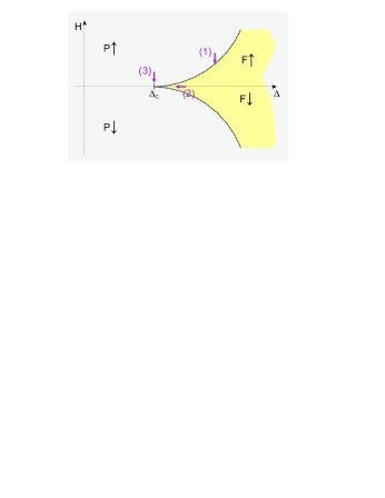
Figure 1: (Color online) Schematic phase-diagram of geometrical clusters of the 2d RFIM as obtained in Ref.[seppala, ]. In the regions, $F\uparrow$ and $F\downarrow$, the majority spin clusters are non-percolating, in $P\uparrow$ and $P\downarrow$, they are percolating. The phase boundary is indicated by dashed lines. The transition along arrow (1) is in the standard percolation universality class. Investigations in this paper are restricted to $H=0$, in particular in the vicinity of the multicritical point along arrow (2).

Some aspects of the structure of the geometrical clusters for a non-zero homogeneous field has been studied in Ref.[seppala, ], see the phase-diagram in Fig.1. For a fixed $\Delta>\Delta_{c}$ the size of the majority spin clusters, $\xi$, is finite for small $H$, but monotonously increasing with increasing $H$. There is a threshold value, $H_{p}(\Delta)$, when the majority spins percolate the sample and for $H>H_{p}(\Delta)$ a finite fraction of the majority spins belongs to the infinite cluster. Close to the percolation point, see arrow $(1)$ in Fig.1, the percolation probability is found to depend on the scaling combination: $L(H_{p}-H)^{\nu_{p}}$, with $\nu_{p}=4/3$ characteristic of the 2d short range percolation transition pointstaufferaharony . Also the fractal dimension of the geometrical clusters at the percolation point is foundseppala to be compatible with that of standard percolationstaufferaharony , $d_{f}=91/48$. According to the numerical results as $\Delta$ is decreased $H_{p}$ tends to zero at $\Delta_{c}$, as $H_{p}\sim(\Delta-\Delta_{c})^{\phi}$, with $\Delta_{c}\approx 1.65$ and $\phi\approx 2.05$.

In the following section we concentrate on the properties of the geometrical clusters at $H=0$. In particular we study the distribution of their mass and introduce and investigate a correlation function, which is associated to geometrical clusters. In these investigations we approach the multicritical point at $\Delta=\Delta_{c}$ and $H=0$ along arrow $(2)$ in Fig.1. With these investigations we want to shied light to the possible geometrical phase transition of the system which takes place at $\Delta_{c}$.

III Results

We have considered the RFIM on $L\times L$ square lattices with periodic boundary conditions in both directions. The strength of the random field is varied in the range $1.2<\Delta<4.$, where the lower limiting value is set by the condition, $L\gg l_{b}(\Delta)$, where the breaking-up length is given in Eq.(3). Using combinatorial optimization algorithm we have calculated the ground state configuration exactly for different finite samples up to a linear size $L=500$. Averages are performed over typically $10000$ different realizations of disorder.

III.1 Distribution of the mass of geometrical clusters

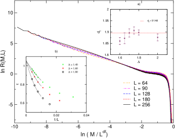
Figure 2: (Color online) Scaling plot of the cumulative distribution of the mass of the geometrical clusters at $\Delta=1.8$, using the fractal dimension of standard percolation. In the inset a) the effective fractal dimension is presented as calculated from the optimal scaling collapse of the curves for different values of $\Delta$. In the inset b) extrapolation of the $\tau$ exponents calculated at different finite systems is presented for $\Delta=1.4$ ($\times$), $\Delta=1.6$ ($+$) and $\Delta=1.8$ ($*$).

We start to study the cumulative distribution of the mass (number of spins), $M$, of the clusters, which is denoted by $R(M,L)$. This measures the fraction of clusters having at least a mass of $M$. According to scaling theory developed for standard percolationstaufferaharony this distribution asymptotically behaves as:

$$R(M,L)=M^{-\tau}\tilde{R}(M/L^{d_{f}})$$ (4)

with a characteristic exponent, $\tau=2/d_{f}$. Thus the only parameter which enters into this expression is the fractal dimension of the clusters, $d_{f}$. This relation is expected to hold at the critical point, where the correlation length, $\xi$, associated to geometrical correlations is divergent. However, Eq.(4) can be a good approximation outside the critical point, too, provided the correlation length, $\xi$, is much larger than the size of the system, $L$. To compute $R(M,L)$ we have performed cluster statistics over $10000$ different random samples and the distributions obtained for different finite systems are scaled together using the relation in Eq.(4). As an illustration in Fig.2 we present the scaled cumulative distribution functions at the specific value, $\Delta=1.8$, in which we used the fractal dimension of standard percolationstaufferaharony , $d_{f}=91/48$. The scaling collapse in Fig.2 is indeed satisfactory. Repeating the same procedure in the range of $1.4<\Delta<2.6$ we have obtained still acceptable data collapse. This means that in this regime the condition $\xi\gg L$ is satisfied and we can conclude that the critical point, $\Delta_{c}$, is also located in this range.

We have also estimated the value of the fractal dimension from the optimal scaling collapse of the curves. For this we have measured the surface of the overlap of the scaled curves for different values of the parameter, $d_{f}$, and at the true fractal dimension the overlap surface is minimal, see in Ref.long2d . The measured effective, i.e. $\Delta$-dependent fractal dimensions are presented in the inset a) of Fig.2. In the range of $1.6<\Delta<2.$ the effective fractal dimensions are approximately constant and consistent with $d_{f}=1.89(2)$. For $\Delta>2.$ the effective $d_{f}$ start to decrease, which is a clear indication that the correlation length is not large enough. The decrease of $d_{f}$ for $\Delta<1.6$, is probably due to the large value of the breaking-up lengths, which starts to approach the size of the system.

From the slope of the curves in Fig.2 in the log-log plot we have measured the exponent, $\tau$, which is defined in Eq.(4). The measured effective exponents for different finite sizes are plotted in the inset b) of Fig.2 for three different values of $\Delta$. Here strong finite-size dependence is visible so that we have to perform an extrapolation procedure in terms of $1/L$. The extrapolated value, as seen in the inset b) of Fig.2, is given by $\tau=1.055(3)$, and this is independent of $\Delta$ we considered. We note that our estimate fits very well to the theoretical value of standard percolationstaufferaharony : $\tau=96/91=1.055$. We can thus conclude that the distribution function of the mass of the geometrical clusters nicely satisfies the scaling prediction in Eq.(4) and the fractal dimension coincides with that of standard percolation.

III.2 Geometrical correlations

Here - using the analogy with ordinary percolation - we introduce the geometrical correlation function, $G(r)$, which is associated to the geometrical clusters. By definition between two spins the geometrical correlation is one, if both spins belong to the same geometrical cluster and zero otherwise. $G(r)$ is then obtained by averaging the correlations over all pairs of spins having a distance, $r$. In the non-critical state, where $\xi<\infty$, the geometrical correlation function is short ranged and expected to decay asymptotically as $G(r)\sim\exp(-r/\xi)$. On the other hand at the critical point the geometrical correlation function has an algebraic decay, $G(r)\sim r^{-\eta}$, where the decay exponent, $\eta$, is related to the fractal dimension as, $\eta=2(d-d_{f})$, through scaling theory.

In practical calculations the system has a finite size, $L$, and in the critical region the geometrical correlation function, $G(r,L)$, is expected to behave asymptotically as: $G(r,L)=r^{-\eta}\tilde{G}(r/L)$. Here the scaling function, $\tilde{G}(y)$, should approach a limiting finite value for small arguments, so that the decay exponent, $\eta$, can be calculated for large finite systems, if $1\ll r\ll L$. As an illustration we shown in Fig.3 the geometrical correlation function for different finite systems in log-log plot for $\Delta=1.8$. Indeed the slope of the curves (of the largest systems) in the region $10<r<40$ is compatible with the theoretical prediction of ordinary percolation: $\eta=5/24=0.208$.

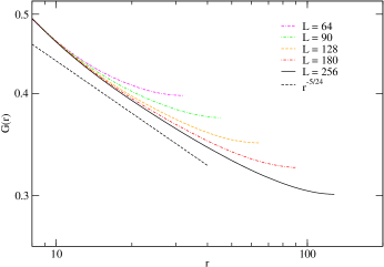
Figure 3: (Color online) Geometrical correlations in a log-log plot for $\Delta=1.8$ and for different system sizes. The theoretical prediction of the asymptotic behavior is indicated by a straight dotted line.

In order to obtain a more accurate estimate of the asymptotic behavior of the geometrical correlation function we measured the correlations between two points of maximal distance, i.e. at $r=L/2$. The maximal distance correlation function defined in this way, $G(L)\equiv G(r=L/2,L)$, is expected to behave in the critical region as: $G(L)=L^{-\eta}\hat{G}(L/\xi)$, thus it is advisable to consider the scaled maximal distance correlation function, $L^{\eta}G(L)=\hat{G}(L/\xi)$. In Fig.4 we have plotted this function for different values of $\Delta$.

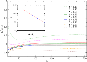
Figure 4: (Color online) Scaled maximal distance geometrical correlations for different values of $\Delta$. The scaled correlations seem to reach a constant limiting value for $\Delta\leq 1.6$, thus here the correlation length is divergent. For stronger random fields the correlations decay to zero, although the correlation length is still a large finite value. Inset: the correlation length as a function of $\Delta-\Delta_{c}$ in a log-log plot. The best fit is obtained with $\Delta_{c}=1.65$ and with an exponent, $\nu=1.98(5)$.

Here one can identify two different regimes as far as the large $L$ dependence of the scaled correlation function is concerned. For strong random fields, $\Delta>\Delta_{c}$, the scaled correlations start to decay to zero, so that the correlation length is finite and the geometrical clusters are non-percolating. On the other hand for weak random fields, $\Delta\leq\Delta_{c}$, the scaled correlations approach a finite limiting value, so that the correlation length is divergent and we are in the phase in which the geometrical clusters are percolating. This conclusion is the same as that obtained through the analysis of the spanning probability in Ref.seppala .

The threshold value of $\Delta_{c}$ can be calculated by analysing the behavior of the correlation length, which can be deduced from the asymptotic dependence: $\hat{G}(L/\xi)\sim\exp[-L/(2\xi)]$. Close to the critical point the correlation length is expected to be in the form: $\xi(\Delta)\sim(\Delta-\Delta_{c})^{-\nu}$. As illustrated in the inset of Fig.4 the best fit is obtained with $\Delta_{c}\approx 1.65$, as in Ref.seppala , whereas for the correlation length critical exponent we have obtained: $\nu=1.98(5)$. This exponent describes the singularity of $\xi$ along arrow (2) in Fig.1. If we want to calculate the divergence of the correlation length at $\Delta_{c}$ but with a small homogeneous field, $H$, i.e. along arrow (3) in Fig.1, we make use of the known result about the critical boundary, $H_{p}\sim(\Delta-\Delta_{c})^{\phi}$. Than from scaling theory we obtain $\xi(H_{p},\Delta_{c})\sim\xi(0,\Delta)\sim H_{p}^{-\tilde{\nu}}$, with $\tilde{\nu}=\nu/\phi=0.97(5)$. We note that this value corresponds to the inverse of the second thermal exponent of tricritical percolationnienhuis : $1/y_{t2}=1$.

III.3 Geometrical correlations in the strip geometry

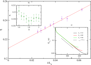
Figure 5: (Color online) Effective decay exponents calculated in periodic strips of width $L_{w}$ through Eq.(7). The dashed straight line indicates extrapolation through $1/L_{w}$. Inset a): Geometrical correlation function at $\Delta=1.8$ in a strip of width $L_{w}=40$ and for different lengths, $L_{1}$. In a semi-log plot the slope of the limiting curve is indicated by a dashed line and given by $1/\xi(L_{w})$. Inset b): $\Delta$-dependence of the effective decay exponent for $L_{w}=40$.

Critical correlations are generally invariant under conformal transformations and conformal invariance has very important consequences in two dimensional systems.cardy One important application of the conformal method is to transform the correlation functions from one geometry to another. In this respect it is of interest if also geometrical correlations are conformally invariant and if one can transform them between different geometries. To answer to this question we have studied geometrical correlations in the RFIM also in the strip geometry. It is known that the infinite plane, described by the complex variable, $z=x+iy$, can be mapped into a periodic strip of width, $L_{w}$, having the complex variable, $w=u+iv$, through the logarithmic conformal transformation:

$$w=\frac{L_{w}}{2\pi}\ln z\;.$$ (5)

Then critical correlations in the plane, $G(z)\sim|z|^{-\eta}$, are transformed into an asymptotic exponential decay along the strip:

$$G_{L_{w}}(u)\sim\exp(-u/\xi(L_{w}))\;,$$ (6)

where the correlation length, $\xi(L_{w})$, is proportional to the width of the strip and given by:

$$\xi(L_{w})=\frac{L_{w}}{\pi\eta}\;.$$ (7)

Thus the proportionality factor contains the decay exponent in the plane, therefore Eq.(7) is called the correlation length - exponent relationluck ; cardy84 .

To check the validity of the correlation length - exponent relation for the RFIM we used strips of widths, $L_{w}=16,20,\dots,40$ and calculated the geometrical correlation function along the strip. The lengths of the strips are taken so large, that the calculated exponential decay in Eq.(6) becomes independent of it. This is illustrated in the inset a) of Fig.5. Generally we went at least up to a length of $16\times L_{w}$ sites. After measuring the correlation length for a given $L_{w}$ we have calculated from Eq.(7) an effective, i.e. $L_{w}$-dependent exponent. This calculation is then repeated for several values of $\Delta$ in the range of $1.4<\Delta<2.0$. For a given $L_{w}$ the $\Delta$-dependence of the exponents are found to be smaller than the actual error of the calculation, as shown in the inset b) of Fig.5. Therefore in Fig.5 we have plotted an average, i.e. $\Delta$-independent exponent as a function of $1/L_{w}$. As seen in this figure the effective exponents have a size dependence and an extrapolation through $1/L_{w}$ leads to the estimate: $\eta=0.210(4)$. This value is in good agreement with the conformal prediction: $\eta=5/24=0.208$. Thus we conclude that our numerical study has confirmed that the correlation length - exponent relation is valid for geometrical correlations in the RFIM.

IV Discussion

In this paper we have considered the RFIM in the square lattice and studied the structure of its ground state at $T=0$. Since in the ground state of the system there is no ferromagnetic long-range order we have focused on the properties of the geometrical clusters consisting of parallel spins. In particular we have investigated the distribution of the mass of the geometrical clusters and studied geometrical correlations, which are associated to geometrical clusters. In agreement with previous investigationsseppala the geometrical clusters are found to have a finite extent for strong random fields, $\Delta>\Delta_{c}$, and being percolating for weak random fields, $\Delta<\Delta_{c}$. For $\Delta\leq\Delta_{c}$ the fractal dimension of geometrical clusters is calculated by different methods and its value is found to be in good agreement with short range percolation. The geometrical correlation function of the system is calculated both in the plane and in the strip geometries. It is shown that the critical geometrical correlation function satisfies both scaling and conformal invariance. In the vicinity of the geometrical critical point the correlation length is found to diverge as: $\xi(\Delta)\sim(\Delta-\Delta_{c})^{-\nu}$, with an exponent, $\nu\approx 2$, whereas at the critical disorder, $\Delta=\Delta_{c}$, the divergence of $\xi(H)$ in the presence of a homogeneous field involves the exponent, $\tilde{\nu}\approx 1$. This latter is characteristic for tricritical percolation.

We note that our study of geometrical clusters in the RFIM is somewhat related to the properties of the random bond Potts model (RBPM) in the large-$q$ limit. As was shown by Cardy and Jacobsenpottstm the interface Hamiltonian of the RFIM separating different types of geometrical clusters, and the interface Hamiltonian of the RBPM separating different types of Fortuin-Kasteleyn clusters, can be mapped into each other. In this respect the absence of long-range order in the RFIM corresponds to the absence of phase coexistence in the RBPM, thus no first-order phase transition in the presence of bond disorder in 2daizenman . Although the interface Hamiltonian of the two problems are equivalent the cluster structure, in particular the value of the fractal dimension is different. For the RBPM the conjectured valueai03 ; long2d for the Fortuin-Kasteleyn clusters, $d_{f}^{P}=(5+\sqrt{5})/4=1.809$, is considerably smaller than that of the RFIM. Thus arguments based on the interface Hamiltonian can be used to study the stability of some phases, but the actual cluster structure is governed by such critical fluctuations which are encoded in the details of the Hamiltonian.

- (1) See, for example, T. Nattermann, in Spin Glasses and Random Fields, ed. A.P. Young (World Scientific, Singapore, 1998).
- (2) See D.P. Belanger, in Spin Glasses and Random Fields, ed. A.P. Young (World Scientific, Singapore, 1998).
- (3) Y. Imry and S.-k. Ma, Phys. Rev. Lett. 35, 1399 (1975).
- (4) A.P. Young, J. Phys. C 10, L257 (1977); G. Parisi and N. Sourlas, Phys. Rev. Lett. 43, 744 (1979).
- (5) D.S. Fisher, Phys. Rev. Lett. 56, 1964 (1986).
- (6) J. Bricmont and A. Kupiainen, Phys. Rev. Lett. 59, 1829 (1987).
- (7) M. Aizenman and J. Wehr, Phys. Rev. Lett. 62, 2503 (1989); erratum 64, 1311 (1990).
- (8) See, for example, D. Stauffer and A. Aharony, Introduction to Percolation Theory, (Taylor and Francis, London) (1992).
- (9) E.T. Seppälä and M.J. Alava, Phys. Rev. E 63, 066109 (2001).
- (10) M.E. Fisher, Physics (Long Island City, N.Y.), 3, 25 (1967).
- (11) For a review, see: A. Coniglio, Nucl. Phys. A681, 451c (2001).
- (12) A. Coniglio, C.R. Nappi, F. Peruggi, and L. Russo, J. Phys. A10, 205 (1977).
- (13) A. L. Stella and C. Vanderzande, Phys. Rev. Lett. 62, 1067 (1989); B. Duplantier and H. Saleur, Phys. Rev. Lett. 63, 2536 (1989); C. Vanderzande, J. Phys. A 25, L75 (1992); W. Janke, and A.M.J. Schakel, Nucl. Phys. B 700, 385 (2004).
- (14) P. W. Kasteleyn and C. M. Fortuin, J. Phys. Soc. Jpn. 46 (Suppl.), 11 (1969).
- (15) H. Müller-Krumbhaar, Phys. Lett. 48A, 459 (1974); D. W. Heermann and D. Stauffer, Z. Phys. B: Condens. Matter 44, 339 (1981); A. Marro and J. Toral, Physica A 122, 563 (1983); Y. Deng, and H.W.J. Blöte, Physical Review E 70, 056132 (2004).
- (16) L. Környei, M. Pleimling, and F. Iglói, Europhys. Lett. 73, 197 (2006); L. Környei, J. Phys. Conf. Ser. 40, 36 (2006).
- (17) J.-Ch. Anglès d’Auriac, M. Preissmann, and R. Rammal, J. Phys. Lett. (France) 46, L173 (1985).
- (18) A.K. Hartmann and H. Rieger, Optimization Algorithms in Physics (Wiley-VCH, Berlin, 2002)
- (19) K. Binder, Z. Phys. B 50, 343 (1983).
- (20) B. Nienhuis, J. Phys. A15, 199 (1982).
- (21) See e.q. J.L. Cardy, in Phase Transitions and Critical Phenomena, Vol. 11, p. 1, edited by J.L. Lebowitz and M.S. Green, (London, Academic) (1987).
- (22) J.H. Luck, J. Phys. A15, L169 (1982).
- (23) J.L. Cardy, J. Phys. A17, L385 (1984).
- (24) J.L. Cardy and J.L. Jacobsen, Phys. Rev. Lett. 79, 4063 (1997).
- (25) J.-Ch. Anglès d’Auriac and F. Iglói, Phys. Rev. Lett. 90, 190601 (2003).
- (26) M.-T. Mercaldo, J-Ch. Anglés d’Auriac, and F. Iglói, Phys. Rev. E 69, 056112 (2004).