Mesoscopic Spin Hall Effect

Abstract

We investigate the spin Hall effect in ballistic chaotic quantum dots with spin-orbit coupling. We show that a longitudinal charge current can generate a pure transverse spin current. While this transverse spin current is generically nonzero for a fixed sample, we show that when the spin-orbit coupling time is large compared to the mean dwell time inside the dot, it fluctuates universally from sample to sample or upon variation of the chemical potential with a vanishing average. For a fixed sample configuration, the transverse spin current has a finite typical value $\simeq e^{2}V/h$, proportional to the longitudinal bias $V$ on the sample, and corresponding to about one excess open channel for one of the two spin species. Our analytical results are in agreement with numerical results in a diffusive system [W. Ren et al., Phys. Rev. Lett. 97, 066603 (2006)] and are further confirmed by numerical simulation in a chaotic cavity.

Introduction. The novel and rapidly expanding field of spintronics is interested in the creation, manipulation, and detection of polarized or pure spin currents spintronics . The conventional methods of doing spintronics are to use magnetic fields and/or ferromagnets as parts of the creation-manipulation-detection cycle, and to use the Zeeman coupling and the ferromagnetic-exchange interactions to induce the spin dependency of transport. More recently, ways to generate spin accumulations and spin currents based on the coupling of spin and orbital degrees of freedom have been explored. Among these proposals, much attention has been focused on the spin Hall effect (SHE), where pure spin currents are generated by applied electric currents on spin-orbit (SO) coupled systems. Originally proposed by Dyakonov and Perel DP71 , the idea was resurrected by Hirsch Hirsch and extended to crystal SO field (the intrinsic SHE) by Sinova et al. macdonald and Murakami et al. murakami . The current agreement is that the SHE vanishes for bulk, $k$-linear SO coupling for diffusive two-dimensional electrons Inoue04 ; halperin ; macdonald2 . This result is however specific to these systems inanc , and the SHE does not vanish for impurity-generated SO coupling, two-dimensional hole systems with either Rashba or Dresselhaus SO coupling, and for finite-sized electronic systems halperin ; inanc . These predictions have been, to some extent, confirmed by experimental observations of edge spin accumulations in electron Kato and hole Wunderlich systems, and electrical detection of spin currents via ferromagnetic leads Valenzuela .

Most investigations of the SHE to date focused on disordered conductors with spin-orbit interaction, where the disorder-averaged spin Hall conductivity was calculated using either the Kubo formalism or a diffusion equation approach Hirsch ; macdonald ; macdonald2 ; loss ; Inoue04 ; halperin ; raimondi ; murakami ; inanc . Few numerical works alternatively used the scattering approach to transport markus to calculate the average spin Hall conductance of explicitly finite-sized samples connected to external electrodes. These investigations were however restricted to tight-binding Hamiltonians with no or weak disorder in simple geometries branislav ; sinova ; sheng . The data of Ref. guo in particular suggest that diffusive samples with large enough SO coupling exhibit universal fluctuations of the spin Hall conductance $G_{\text{sH}}$ with ${\rm rms}[G_{\text{sH}}]\approx 0.18e/4\pi$. These numerical investigations call for an analytical theory of the SHE in mesoscopic systems. It is the purpose of this article to provide such a theory.

We analytically investigate the DC spin Hall effect in mesoscopic cavities with SO coupling. We calculate both the ensemble-average and the fluctuations of the transverse spin current generated by a longitudinal charge current. Our approach is based on random matrix theory (RMT) carlormp , and is valid for ballistic chaotic and mesoscopic diffusive systems at low temperature, in the limit when the spin-orbit coupling time is much shorter than the mean dwell time of the electrons in the cavity, $\tau_{\rm so}\ll\tau_{\rm dwell}$ caveat1 . We show that while the transverse spin current is generically nonzero for a typical sample, its sign and amplitude fluctuate universally, from sample to sample or upon variation of the chemical potential with a vanishing average. We find that for a typical ballistic chaotic quantum dot, the transverse spin current corresponds to slightly less than one excess open channel for one of the two spin species. These analytical results are confirmed by numerical simulations for a stroboscopic model of a ballistic chaotic cavity.

Scattering approach. We consider a ballistic chaotic quantum dot coupled to four external electrodes via ideal point contacts, each with $N_{i}$ open channels ($i=1,\ldots 4$). The geometry is sketched in Fig. 1. Spin-orbit coupling exists only inside the dot, and the electrochemical potentials in the electrodes are spin-independent. A bias voltage $V$ is applied between the longitudinal electrodes labeled 1 and 2. The voltages $V_{3}$ and $V_{4}$ are set such that no net charge current flows through the transverse electrodes 3 and 4. We will focus on the magnitude of the spin current through electrodes 3 and 4, in the limit when the openings to the electrodes are small enough, and the spin-orbit coupling strong enough that $\tau_{\rm so}\ll\tau_{\rm dwell}$.

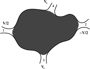
Figure 1: Ballistic quantum dot connected to four electrodes. The longitudinal bias $V$ induces a charge current through terminals 1 and 2, while the voltages $V_{3,4}$ are adjusted such that no charge current flows through the transverse leads 3 and 4. Spin-orbit coupling is active only in the gray region.

We write the spin-resolved current through the $i$-th electrode as markus

$$I_{i}^{\sigma}=\frac{e^{2}}{h}\sum_{j,\sigma^{\prime}}T^{\sigma,\sigma^{\prime}}_{ij}(V_{i}-V_{j}).$$ (1)

The spin-dependent transmission coefficients are obtained by summing over electrode channels

$$T^{\sigma,\sigma^{\prime}}_{i,j} = \sum_{m\in i}\sum_{n\in j}|t_{m,\sigma;n,\sigma^{\prime}}|^{2},$$ (2)

i.e. $t_{m,\sigma;n,\sigma^{\prime}}$ is the transmission amplitude for an electron initially in a spin state $\sigma^{\prime}$ in channel $n$ of electrode $j$ to a spin state $\sigma$ in channel $m$ of electrode $i$. The transmission amplitudes $t$ are the elements of the $2N_{T}\times 2N_{T}$ scattering matrix $S$, with $N_{T}=\sum_{i=1}^{4}N_{i}$.

We are interested in the transverse spin currents $I_{i}^{(z)}=I_{i}^{\uparrow}-I_{i}^{\downarrow}$, $i=3,4$, under the two constraints that (i) charge current vanishes in the transverse leads, $I_{i}^{\uparrow}+I_{i}^{\downarrow}=0$, $i=3,4$ and (ii) the charge current is conserved, $I_{1}=-I_{2}=I$. From Eq. (1), transport through the system is then described by the following equation

$$\left(\begin{array}[]{c}2J\\ J_{3}^{(z)}\\ J_{4}^{(z)}\end{array}\right) = \left(\begin{array}[]{ccc}2N_{1}-{\mathcal{T}}_{11}^{(0)}+2N_{2}-{\mathcal{T}}_{22}^{(0)}+{\mathcal{T}}_{12}^{(0)}+{\mathcal{T}}_{21}^{(0)}&{\mathcal{T}}_{23}^{(0)}-{\mathcal{T}}_{13}^{(0)}&{\mathcal{T}}_{24}^{(0)}-{\mathcal{T}}_{14}^{(0)}\\ {\mathcal{T}}_{32}^{(z)}-{\mathcal{T}}_{31}^{(z)}&-{\mathcal{T}}_{33}^{(z)}&-{\mathcal{T}}_{34}^{(z)}\\ {\mathcal{T}}_{42}^{(z)}-{\mathcal{T}}_{41}^{(z)}&-{\mathcal{T}}_{43}^{(z)}&-{\mathcal{T}}_{44}^{(z)}\end{array}\right)\left(\begin{array}[]{c}1/2\\ \tilde{V}_{3}\\ \tilde{V}_{4}\end{array}\right),$$ (12)

where the transverse voltages (in units of $V$) read

$$\tilde{V}_{3} =\frac{1}{2}\frac{{\mathcal{T}}_{34}^{(0)}({\mathcal{T}}_{42}^{(0)}-{\mathcal{T}}_{41}^{(0)})+(2N_{4}-{\mathcal{T}}_{44}^{(0)})({\mathcal{T}}_{32}^{(0)}-{\mathcal{T}}_{31}^{(0)})}{{\mathcal{T}}_{34}^{(0)}{\mathcal{T}}_{43}^{(0)}-(2N_{3}-{\mathcal{T}}_{33}^{(0)})(2N_{4}-{\mathcal{T}}_{34}^{(0)})},$$ (13a)

$$\tilde{V}_{4} =\frac{1}{2}\frac{{\mathcal{T}}_{43}^{(0)}({\mathcal{T}}_{32}^{(0)}-{\mathcal{T}}_{31}^{(0)})+(2N_{3}-{\mathcal{T}}_{33}^{(0)})({\mathcal{T}}_{42}^{(0)}-{\mathcal{T}}_{41}^{(0)})}{{\mathcal{T}}_{34}^{(0)}{\mathcal{T}}_{43}^{(0)}-(2N_{3}-{\mathcal{T}}_{33}^{(0)})(2N_{4}-{\mathcal{T}}_{34}^{(0)})},$$ (13b)

and we defined the dimensionless currents $I=e^{2}VJ/h$. We introduced generalized transmission probabilities

$$\mathcal{T}_{ij}^{(\mu)}=\sum_{m\in i,n\in j}{\rm Tr}[(t_{mn})^{\dagger}\sigma^{(\mu)}t_{mn}],\;\;\;\;\mu=0,x,y,z,$$ (14)

where $\sigma^{(\mu)}$ are Pauli matrices ($\sigma^{(0)}$ is the identity matrix) and one traces over the spin degree of freedom.

Random matrix theory. We calculate the average and fluctuations of the transverse spin currents $J_{i}^{(\mu)}$, $\mu=x,y,z$ within the framework of RMT. Accordingly, we replace the scattering matrix $S$ by a random unitary matrix, which, in our case of a system with time reversal symmetry (absence of magnetic field) and totally broken spin rotational symmetry (strong spin-orbit coupling), has to be taken from the circular symplectic ensemble (CSE) carlormp ; caveat2 ; Ale01 ; Bro02 . We rewrite the generalized transmission probabilities $\mathcal{T}_{ij}^{(\mu)}$ as a trace over $S$

$$\mathcal{T}_{ij}^{(\mu)} =\text{Tr}\,[Q_{i}^{(\mu)}SQ_{j}^{(0)}S^{\dagger}],$$ (15)

$$[Q_{i}^{(\mu)}]_{m\alpha,n\beta} =\begin{cases}\delta_{mn}\leavevmode\nobreak\ \sigma^{(\mu)}_{\alpha\beta},&\sum_{j=1}^{i-1}N_{j}<m\leq\sum_{j=1}^{i}N_{j},\\ 0,&\text{otherwise}.\end{cases}$$

Here, $m$ and $n$ are channel indices, while $\alpha$ and $\beta$ are spin indices. The trace is taken over both set of indices.

Averages, variances, and covariances of the generalized transmission probabilities (15) over the CSE can be calculated using the method of Ref. Bro96 . For the average transmission probabilities, we find

$$\langle\mathcal{T}^{(\mu)}_{ij}\rangle=\frac{2\delta_{\mu 0}}{N_{T}-1/2}\left(N_{i}N_{j}-\frac{1}{2}N_{i}\delta_{ij}\right),$$ (16)

while variances and covariances are given by

$$\langle\delta\mathcal{T}_{ij}^{(\mu)}\delta\mathcal{T}_{kl}^{(\nu)}\rangle=\frac{4\delta_{\mu\nu}}{N_{T}(2N_{T}-1)^{2}(2N_{T}-3)}\Big{\{}N_{i}N_{j}(N_{T}-1)(2N_{T}-1)(\delta_{ik}\delta_{jl}+\delta_{il}\delta_{jk}\delta_{\mu 0})$$

$$+(N_{i}N_{k}\delta_{ij}\delta_{kl}-2N_{i}N_{k}N_{l}\delta_{ij}-2N_{i}N_{j}N_{k}\delta_{kl}+4N_{i}N_{j}N_{k}N_{l})\delta_{\mu 0}-N_{i}N_{T}(2N_{T}-1)\delta_{ijkl}+(2N_{T}-1)\times$$ (17)

$$\Big{[}N_{i}N_{l}\delta_{ijk}+N_{i}N_{k}\delta_{ijl}\delta_{\mu 0}+N_{i}N_{j}(\delta_{ikl}+\delta_{jkl}\delta_{\mu 0})-N_{i}N_{j}N_{l}(\delta_{ik}+\delta_{jk}\delta_{\mu 0})-N_{i}N_{j}N_{k}\delta_{\mu 0}(\delta_{il}+\delta_{jl})\Big{]}\Big{\}},$$

where $\delta\mathcal{T}_{ij}^{(\mu)}=\mathcal{T}_{ij}^{(\mu)}-\langle\mathcal{T}_{ij}^{(\mu)}\rangle$.

Because the transverse potentials $\tilde{V}_{3,4}$ are spin-independent, they are not correlated with $\mathcal{T}^{(\mu)}_{ij}$. Additionally taking Eq. (16) into account, one concludes that the average transverse spin current vanishes ($i=3,4$),

$$\langle J_{i}^{(\mu)}\rangle=\frac{1}{2}\langle{\mathcal{T}}_{i2}^{(\mu)}-{\mathcal{T}}_{i1}^{(\mu)}\rangle-\sum_{j=3,4}\langle{\mathcal{T}}_{ij}^{(\mu)}\rangle\langle\tilde{V}_{j}\rangle=0.$$ (18)

However, for a given sample at a fixed chemical potential $J_{i}^{(\mu)}$ will in general be finite. We thus calculate $\text{var}\;[J_{i}^{(\mu)}]$. We first note that $\langle\tilde{V}_{3,4}\rangle/V=(N_{1}-N_{2})/2(N_{1}+N_{2})$, and that $\text{var}\;[\tilde{V}_{3,4}]$ vanishes to leading order in the inverse number of channels. One thus has

$$\text{var}\;[J_{i}^{(\mu)}]=\frac{1}{4}\sum_{j=1,2}\text{var}[\mathcal{T}_{ij}^{(\mu)}]-\frac{1}{2}\,\text{covar}[\mathcal{T}_{i1}^{(\mu)},\mathcal{T}_{i2}^{(\mu)}]$$ (19)

$$+\sum_{j=3,4}\Big{\{}\text{var}[\mathcal{T}_{ij}^{(\mu)}]\langle\tilde{V}_{j}\rangle^{2}+\text{covar}[\mathcal{T}_{i1}^{(\mu)}-\mathcal{T}_{i2}^{(\mu)},\mathcal{T}_{ij}^{(\mu)}]\langle\tilde{V}_{j}\rangle\Big{\}}$$

$$+2\,\text{covar}[\mathcal{T}_{i3}^{(\mu)},\mathcal{T}_{i4}^{(\mu)}]\langle\tilde{V}_{3}\rangle\langle\tilde{V}_{4}\rangle.$$

From Eq. (Mesoscopic Spin Hall Effect) it follows that

$$\text{var}\;[J_{i}^{(\mu)}]=\frac{4N_{i}N_{1}N_{2}(N_{T}-1)}{N_{T}(2N_{T}-1)(2N_{T}-3)(N_{1}+N_{2})}.$$ (20)

Eqs. (18) and (20) are our main results. They show that, while the average transverse spin current vanishes, it exhibits universal sample-to-sample fluctuations. The origin of this universality is the same as for charge transport carlormp , and relies on the fact expressed in Eq. (Mesoscopic Spin Hall Effect) that to leading order, spin-dependent transmission correlators do not scale with the number of channels. The spin current carried by a single typical sample is given by ${\rm rms}[J_{i}^{(\mu)}]\times e^{2}V/h$, and is thus of order $e^{2}V/h$ in the limit of large number of channels. In other words, for a given sample, one spin species has of order one more open transport channel than the other one. For a fully symmetric configuration, $N_{i}\equiv N$, the spin current fluctuates universally for large $N$, with ${\rm rms}[I_{3}^{z}]\simeq(e^{2}V/h)/\sqrt{32}$. This translates into universal fluctuations of the transverse spin conductance with ${\rm rms}[G_{\rm sH}]=(e/4\pi\sqrt{32})\approx 0.18(e/4\pi)$ in agreement with Ref. guo .

Numerical simulation. In the diffusive setup of Ref. guo the universal regime is not very large and thus it is difficult to unambiguously identify it. We therefore present numerical simulations in chaotic cavities to further illustrate our analytical predictions (18) and (20).

We model the electronic dynamics inside a chaotic ballistic cavity by the spin kicked rotator Sch89 ; Bar05 , a one-dimensional quantum map which we represent by a $2M\times 2M$ Floquet (time-evolution) matrix Izr90

$$\mathcal{F}_{ll^{\prime}} =(\Pi UXU^{\dagger}\Pi)_{ll^{\prime}},\quad l,l^{\prime}=0,1,\ldots,M-1,$$ (21a)

$$\Pi_{ll^{\prime}} =\delta_{ll^{\prime}}e^{-i\pi(l+l_{0})^{2}/M}\sigma_{0},$$ (21b)

$$U_{ll^{\prime}} =M^{-1/2}e^{-i2\pi ll^{\prime}/M}\sigma_{0},$$ (21c)

$$X_{ll^{\prime}} =\delta_{ll^{\prime}}e^{-i(M/4\pi)V(2\pi l/M)}.$$ (21d)

The matrix size $2M=2L/\lambda_{F}\gg 1$ is given by twice the ratio of the linear system size to the Fermi wavelength. The matrix $X$ with

$$V(p)=K\cos p\,\sigma_{0}+K_{\text{so}}(\sigma_{x}\sin 2p+\sigma_{z}\sin p).$$ (22)

corresponds to free SO coupled motion interrupted periodically by kicks described by the matrix $\Pi$, corresponding to scattering off the boundaries of the quantum dot. In this form, the model is time-reversal symmetric, and the parameter $l_{0}$ ensures that no additional symmetry exists in the system. The map is classically chaotic for kicking strength $K\gtrsim 7.5$, and $K_{\text{so}}$ is related to the SO coupling time $\tau_{\text{so}}$ (in units of the stroboscopic period) through $\tau_{\text{so}}=32\pi^{2}/K_{\text{so}}^{2}M^{2}$ Bar05 . From (21), we construct the quasienergy-dependent scattering matrix fyodorov

$$S(\varepsilon)=P[e^{-i\varepsilon}-{\mathcal{F}}(1-P^{T}P)]^{-1}{\mathcal{F}}P^{T},$$ (23)

with $P$ a $2N_{T}\times 2M$ projection matrix

$$P_{k\alpha,k^{\prime}\beta}=\begin{cases}\delta_{\alpha\beta}&\text{if }k^{\prime}=l^{(k)},\\ 0&\text{otherwise}.\end{cases}$$ (24)

The $l^{(k)}$ ($k=1,2,\ldots,2N_{T}$, labels the modes) give the position in phase space of the attached leads. The mean dwell time $\tau_{\text{dwell}}$ (in units of the stroboscopic period) is given by $\tau_{\text{dwell}}=M/N_{T}$. At large enough SO coupling, this model has been shown to exhibit the universality of the CSE. We refer the reader to Ref. Bar05 for further details on the model.

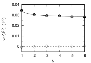
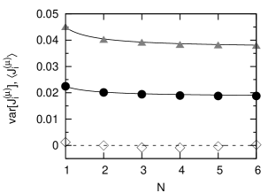
Figure 2: Average and variance of the transverse spin current vs. the number of modes. Top panel: longitudinally symmetric configuration with $N_{1}=N_{2}=2N_{3}=2N_{4}=2N$; bottom panel: longitudinally asymmetric configuration with $N_{2}=N_{4}=2N_{1}=2N_{3}=2N$. In both cases the total number of modes $N_{T}=6N$. The solid (dashed) lines give the analytical prediction (18) [(20)] for the mean (variance) of the spin currents. Empty diamonds correspond to $\langle J_{i}^{(\mu)}\rangle$, circles to $\text{var}\;[J_{3}^{(\mu)}]$ and triangles to $\text{var}\;[J_{4}^{(\mu)}]$.

Averages were performed over 35 values of $K$ in the range $41<K<48$, 25 values of $\varepsilon$ uniformly distributed in $0<\varepsilon<2\pi$, and 10 different lead positions $l^{(k)}$. We set the strength of $K_{\rm so}$ such that $\tau_{\text{so}}=\tau_{\text{dwell}}/1250$, and fixed values of $M=640$ and $l_{0}=0.2$.

Our numerical results are presented in Fig. 2. Two cases were considered, the longitudinally symmetric ($N_{1}=N_{2}$) and asymmetric ($N_{1}\neq N_{2}$) configurations. In both cases, the numerical data fully confirm our predictions that the average spin current vanishes and that the variance of the transverse spin current is universal, i.e. it does not depend on $N$ for large enough value of $N$. In the asymmetric case $N_{4}=2N_{3}$, the variance of the spin current in lead 4 is twice as big as in lead 3, giving further confirmation to Eq. (20).

Conclusion. We have calculated the average and mesoscopic fluctuations of the transverse spin current generated by a charge current through a chaotic quantum dot with SO coupling. We find that, from sample to sample, the spin current fluctuates universally around zero average. In particular, for a fully symmetric configuration $N_{i}\equiv N$, this translates into universal fluctuations of the spin conductance with ${\rm rms}[G_{\rm sH}]=(e/4\pi\sqrt{32})\approx 0.18(e/4\pi)$. This analytically establishes the universality observed numerically in Ref. guo .

We thank C.W.J. Beenakker for valuable comments on the manuscript. JHB acknowledges support by the European Community’s Marie Curie Research Training Network under contract MRTN-CT-2003-504574, Fundamentals of Nanoelectronics. IA acknowledges support by the Deutsche Forschungsgemeinschaft within the cooperative research center SFB 689 “Spin phenomena in low dimensions” and NSERC Canada discovery grant number R8000.

References

- (1) I. Zutić et al., Rev. Mod. Phys. 76, 323 (2004).
- (2) M.I. Dyakonov and V.I. Perel, Sov. Phys. JETP Lett. 13, 467 (1971); Phys. Lett. A 35,459 (1971).
- (3) J. E. Hirsch, Phys. Rev. Lett. 83, 1834 (1999)
- (4) J. Sinova et al., Phys. Rev. Lett. 92, 126603 (2004).
- (5) S. Murakami, Phys. Rev. B 69, 241202(R) (2004).
- (6) J.-I. Inoue, G.E.W. Bauer, and L.W. Molenkamp, Phys. Rev. B 70, 041303(R) (2004).
- (7) E.G. Mishchenko, A.V. Shytov, and B.I. Halperin, Phys. Rev. Lett. 93, 226602 (2004).
- (8) A.A. Burkov, A.S. Núñez, and A.H. MacDonald, Phys. Rev. B 70, 155308 (2004).
- (9) I. Adagideli and G.E.W. Bauer, Phys. Rev. Lett. 95, 256602 (2005).
- (10) Y.K. Kato et al., Science 306, 1910 (2004); V. Sih et al., Nature Phys. 1, 31-35 (2005).
- (11) J. Wunderlich et al., Phys. Rev. Lett. 94, 047204 (2005);
- (12) E. Saitoh et al., Appl. Phys. Lett. 88, 182509 (2006); S.O. Valenzuela and M. Tinkham, Nature 442, 176 (2006); T. Kimura et al., cond-mat/0609304.
- (13) J. Schliemann and D. Loss, Phys. Rev. B 71, 085308 (2005).
- (14) R. Raimondi and P. Schwab, Phys. Rev. B 71, 033311 (2005).
- (15) M. Büttiker, Phys. Rev. Lett. 57, 1761 (1986).
- (16) B.K. Nikolić, L.P. Zârbo, and S. Souma, Phys. Rev. B 72, 75361 (2005).
- (17) E.M. Hankiewicz, L.W. Molenkamp, T. Jungwirth, and J. Sinova, Phys. Rev. B 70, 241301(R) (2004).
- (18) L. Sheng, D.N. Sheng, and C.S. Ting, Phys. Rev. Lett. 94, 016602 (2005).
- (19) W. Ren, Z. Qiao, J. Wang, Q. Sun, and H. Guo, Phys. Rev. Lett. 97, 066603 (2006).
- (20) C. W. J. Beenakker, Rev. Mod. Phys. 69, 731 (1997).
- (21) It is at present unclear to us whether the validity of RMT for the spin Hall effect in mesoscopic diffusive samples requires averaging over lead positions, in addition to disorder averaging.
- (22) We assume that the SO coupling parameters are sufficiently nonuniform, so that SO cannot be removed from the Hamiltonian by a gauge transformation, see : Ale01 ; Bro02 .
- (23) I. L. Aleiner and V. I. Fal’ko, Phys. Rev. Lett. 87, 256801 (2001).
- (24) P. W. Brouwer, J. N. H. J. Cremers, and B. I. Halperin, Phys. Rev. B 65, 081302(R) (2002).
- (25) P. W. Brouwer and C. W. J. Beenakker, J. Math. Phys. 37, 4904 (1996).
- (26) R. Scharf, J. Phys. A 22, 4223 (1989).
- (27) J. H. Bardarson, J. Tworzydło, and C. W. J. Beenakker, Phys. Rev. B 72, 235305 (2005).
- (28) F. M. Izrailev, Phys. Rep. 196, 299 (1990).
- (29) Y.V. Fyodorov and H.-J. Sommers, JETP Lett. 72, 422 (2000).