Energy Level Statistics of Quantum Dots

Abstract

We investigate the charging energy level statistics of disordered interacting electrons in quantum dots by numerical calculations using the Hartree approximation. The aim is to obtain a global picture of the statistics as a function of disorder and interaction strengths. We find Poisson statistics at very strong disorder, Wigner-Dyson statistics for weak disorder and interactions, and a Gaussian intermediate regime. These regimes are as expected from previous studies and fundamental considerations, but we also find interesting and rather broad crossover regimes. In particular, intermediate between the Gaussian and Poisson regimes we find a two-sided exponential distribution for the energy level spacings. In comparing with experiment, we find that this distribution may be realized in some quantum dots.

1 Introduction

Understanding energy level statistics (ELS) of quantum many-body systems is a fundamental and intriguing challenge. Wigner first proposed the statistical method in order to understand the excitation energies of nuclei, and developed the mathematics of random matrix theory (RMT) to do the calculations [1]. This idea has been very successful in elucidating experimental data in nuclear spectroscopy [2]. The advent of artificially constructed finite interacting quantum systems provides an opportunity to test these ideas again [3]. Quantum dots are the system of choice today, and indeed RMT is useful in describing transport and excitation energies in dots [4]. Dots have the additional feature that the particle number can be changed in a controlled fashion, and one can investigate a somewhat different quantity, the change in ground state energy when a particle is added to the dot. This distribution of level spacings when the particle number is changed will be termed the charging energy level statistics (CELS). Surprisingly, these statistics of this quantity do not follow RMT at all [5].

The CELS is measured as follows. In the Coulomb blockade regime, the conductance of a dot is highly resonant, with a sharp peak when the chemical potential difference of the leads is equal to the difference $E_{G}(N+1)-E_{G}(N)$, where $E_{G}(N)$ is the total ground state energy of the dot with $N$ particles. Since the particle number can be varied by adjusting the gate voltage, the quantity $\Delta_{2}(N)\equiv E_{G}(N+1)-2E_{G}(N)+E_{G}(N-1)$ can be measured by recording the spacing of adjacent conductance peaks on the graph of conductance vs. gate voltage. $\Delta_{2}$ fluctuates as the particle number is varied. By measuring it for many different dot fillings, a probability distribution $P(\Delta_{2})$ can be built up, and it is this distribution that is compared to theory.

The simplest way to apply RMT to the CELS is via the constant interaction model, which goes as follows [6]. Let the dot have charge $Q=-Ne$ and capacitance $C$. Now assume that one may separate the energy into a non-fluctuating (“constant”) energy of interaction $E_{C}(N)=Q^{2}/2C$ and a fluctuating part $E_{f}(N)$. Then

$$\Delta_{2}(N) = (e^{2}/2C)[(N+1)^{2}-2N^{2}+(N-1)^{2}]$$

$$+E_{f}(N+1)-2E_{f}(N)+E_{f}(N-1)$$

$$= e^{2}/C+E_{f}(N+1)-2E_{f}(N)+E_{f}(N-1).$$

Further assume that RMT can be applied to $E_{f}(N)$ and the conclusion is that $\Delta_{2}(N)-e^{2}/C$ should follow Wigner-Dyson statistics. That is, if $\Delta_{2}(N)$ is measured for many $N$ and a histogram is built up, the shape of the histogram, when normalized to unit area, should converge (to a very good approximation) to the form

$$P_{WD}(\Delta_{2}-e^{2}/C)=\left\{\begin{array}[]{l}0,\,\,\,\,\textrm{ if }\Delta_{2}-e^{2}/C<0\\ \frac{\pi}{2s^{2}}\left(\Delta_{2}-e^{2}/C\right)\exp\left[\frac{-\pi}{4}(\frac{\Delta_{2}-e^{2}/C}{s})^{2}\right],\,\textrm{otherwise.}\end{array}\right.$$ (1)

This is sometimes called the CI (constant interaction) + RMT model. The prediction of Eq. (1) is in stark contradiction to experiments on the CELS, which show a $P(x)$ that is usually approximately Gaussian instead of having the asymmetric shape predicted by Eq. (1) [5].

This basic discrepancy was resolved by the work of Cohen et al. [7]. These authors solved the Hartree-Fock equations for a finite disordered interacting system of charges on a lattice. This produced a Gaussian shape for $P(x)$. The origin of this distribution is the Hartree term in the total energy. The Hartree potential at any given site is a sum of random variables, the charges at all the other sites weighted by their inverse distance to the given site. Application of the central limit theorem to this potential then yields the Gaussian form for the CELS. By making an experimentally-guided estimate of the parameters in the model, Cohen et al. also found agreement between theory and the experimental data of Sivan et al. [5] for the width of the distribution.

However, there remain unanswered questions. Some are experimental. As we shall show in detail below, the most extensive data on $P(x)$ [8] show marked deviations from the Gaussian shape. In particular, there are broad tails in the distribution. Furthermore, other experiments [9]  show some asymmetry in the distribution function, indicating that the Gaussian is not universal.

There are also purely theoretical issues to be resolved. RMT is certainly valid in regimes where the interaction is weak, as it is known to be correct for non interacting systems. This means that there should be a crossover regime from Wigner-Dyson to Gaussian statistics as the strength of the interaction is increased and this has been seen in numerical studies [4], [10]. We analyze this in some more detail by finding the crossover point in the presence of disorder with variable strength.  Also, it has been shown by Shklovskii et al. [11] that Wigner-Dyson statistics do not apply near the Fermi energy of Anderson insulators. In this case the energy levels follow Poisson statistics.  Thus, if the disorder dominates, we have yet a third kind of statistics, again with crossovers that are in need of investigation. In this regard, it is interesting to note recent work by Berkovits et al., who find a crossover from Wigner-Dyson to Poisson statistics as a function of interaction strength in the energy of the first excited state of dots [12]. Alhassid et al. have seen the crossover from Gaussian to Wigner-Dyson statistics, in a more generical model of a dot, valid at small dimensionless resistance [13].

In this work, we take a synthetic approach to answer these experimental and theoretical questions, in the hope of arriving at a global understanding of the CELS of quantum dots. In Sec. 2, we introduce a model that includes interactions, disorder and hopping. We first examine the classical limit of the model and then extend the arguments to the quantum case. The qualitative results are summarized by means of a conjectured “statistics plot”. In Sec. 3, we present the results of numerical simulations to bolster the theoretical conclusions and make them somewhat more quantitative. The final results are presented in Sec. 4. Comparison to experiment is made in Sec. 5, and our conclusions are in Sec. 6.

2 Model

Our model of a dot is a system of $N$ interacting electrons on a disordered lattice of $N_{s}$ sites: the Anderson Hamiltonian with long-range Coulomb interactions:

$$\mathcal{H}^{\prime}=\sum_{i}^{N_{s}}u_{i}^{\prime}n_{i}-t^{\prime}\sum_{\left\langle ij\right\rangle}^{N_{s}}\left(c_{i}^{\dagger}c_{j}+c_{j}^{\dagger}c_{i}\right)+e^{2}\sum_{i\neq j}\frac{n_{i}n_{j}}{\left|\vec{R}_{i}-\vec{R}_{j}\right|}.$$ (2)

In this equation, $i$ labels the sites of a finite square lattice. The sites are located at $\vec{R}_{i}=(ma,na)$, where $m$ and $n$ are integers: $1\leq m\leq L$ and $1\leq n\leq L.$  $\left\langle ij\right\rangle$ is a nearest-neighbor pair, $n_{i}=c_{i}^{\dagger}c_{i}$ is the number operator, and $\varepsilon_{i}^{\prime}$ are the site energies. The $u_{i}^{\prime}$ are drawn from a probability distribution $P(\varepsilon_{i}^{\prime})$ of width $W$:

$$P(u_{i}^{\prime})=\left\{\begin{array}[]{ccl}1/W\,^{\prime},&\textrm{for}&\left|u_{i}^{\prime}\right|<W^{\prime}/2\\ 0,&\textrm{for}&\left|u_{i}^{\prime}\right|>W^{\prime}/2\end{array}\right..$$ (3)

As we explain below, we will find the ground state of this Hamiltonian numerically in the Hartree approximation. Since this approximation does not respect the exclusion principle, double occupancy of sites is allowed.  We suppress this by adding an energy $U=4e^{2}/a$ for each doubly occupied site. We will briefly consider the effect of varying $U$ below.

The model has three parameters $t^{\prime},W^{\prime},$ and $e^{2}/a$.  Our main interest lies in the energy level statistics. These statistics can only depend on two parameters, since one of the three can be scaled out.  We choose $e^{2}/a$ as our energy unit and so define the dimensionless quantities $\mathcal{H}=\mathcal{H}^{\prime}a/e^{2},$ $t=t^{\prime}a/e^{2},$ $\vec{r}_{i}=\vec{R}_{i}/a$, and $W=W^{\prime}a/e^{2}$, leading to

$$\mathcal{H}=\sum_{i}^{N_{s}}u_{i}n_{i}-t\sum_{\left\langle ij\right\rangle}^{N_{s}}\left(c_{i}^{\dagger}c_{j}+c_{j}^{\dagger}c_{i}\right)+\sum_{i\neq j}\frac{n_{i}n_{j}}{\left|\vec{r}_{i}-\vec{r}_{j}\right|}$$ (4)

and

$$P(u_{i})=\left\{\begin{array}[]{ccc}1/W&\textrm{for}&\left|u_{i}\right|<W/2\\ 0&\textrm{for}&\left|u_{i}\right|>W/2\end{array}\right..$$ (5)

Our model of the dot is not the most general. However, we believe it is the simplest one that combines the three essential features of the problem: disorder, interaction, and hopping. It takes the simplest possible form for the disorder, the simplest non-interacting band structure, and the simplest long-range interaction. We shall have occasion to briefly investigate some elaborations of the model such as different dot shapes and different boundary conditions. It is generally believed that the Anderson model is sufficiently general to capture all the qualitative features of many physical properties having to do with disorder, localization being the prime example. Given the intimate connection between localization and level statistics, it seems plausible that this model is a good starting point for our problem.

The chief difficulties in the numerical calculations are the necessities of averaging over many realizations of the disorder and converging accurately to the authentic ground state. In order to accomplish these two objectives, we are forced to neglect the spin degree of freedom. This is undesirable, particularly in view of suggestions that energy-level pairing might take place, leading to bimodal distributions for the CELS. We only note that this phenomenon is apparently absent in most experiments, and also in most of the numerical work done previously. Since we will do calculations in the Hartree approximation, we must also specify the onsite interaction, which is taken as $U=4$. We discuss this choice further below.

To understand the level statistics of a particular dot, we model it by Eq. (4) and then situate it on a plot of disorder versus hopping strength: $W$ vs. $t$, and our task is to figure out the physics of all the regions of the $W-t$ plane. We shall refer to this diagram as the “statistics plot”. The motivation for plotting in this way is that the limiting regimes of the CELS can easily be picked out. Let us discuss the theoretical expectations for these regimes in turn.

The classical regime is defined by $t=0,$which is the vertical axis of the statistics plot. Far out along this vertical axis of the statistics plot, $W\rightarrow\infty$ and the disorder is dominant, and we can neglect both hopping and interactions. Each electron sits on a single site, and the sites $i$ are filled up in the order of $u_{i},$ from lowest to highest.  The ground state energy is given by

$$E(N)=\sum_{i=1}^{N}u_{i},$$ (6)

where the $u_{i}$ are indexed such that $u_{1}<u_{2}<u_{3}<\cdot\cdot\cdot$  . Also

$$\Delta_{2}=E_{G}(N+1)-2E_{G}(N)+E_{G}(N-1)=u_{N+1}-u_{N}.$$ (7)

This leads to Poisson statistics, essentially independent of the statistics chosen for the $u_{i}$:

$$P_{P}(\Delta_{2})=\left\{\begin{array}[]{ccc}e^{-\Delta_{2}/s}/s&\textrm{if}&\Delta_{2}>0\\ 0&\textrm{if}&\Delta_{2}<0\end{array}\right.$$ (10)

and note that this is properly normalized. The capacitance $C$, which gives a rigid shift $e^{2}/C$ in the distribution, is effectively infinite owing to the absence of interactions in this limit. Because of the vanishing of $P_{P}$ at negative arguments, this is also an asymmetric distribution.

To understand the classical regime at weak disorder $W<<1$, it is necessary to estimate the potential fluctuations. Consider a set of $N$ charges on the lattice. In the absence of disorder ($W=0$), they will be distributed in space in such a way as to make the entire dot into an equipotential surface, up to atomic-scale graininess, which also gives graininess to the Coulomb potential. If we add a small amount of disorder in an infinite system, we expect that the site where the next charge goes to be determined entirely by the graininess in the Coulomb potential and the weak randomness coming from the very small disorder in site energies. Thus the width of the distribution $P(\Delta_{2},W),$ which we shall denote by $\sigma_{X}$ has a small intercept on the $W$ axis and is linear in $W$: $\sigma_{X}(\Delta_{2},W)=P_{0}+\beta W$, the first term coming from the graininess and the second from the disorder. This process clearly leads to Gaussian statistics, as the site energies are chosen at random and their sum is the total energy. As detailed below, we find empirically that the atomic-scale graininess is smaller than one might expect.

Thus at small disorder we have Gaussian CELS and at large disorder we have Poisson CELS. At what value of $W$  does the crossover occur?

Increasing the amount of disorder from small values we will find that some charges, on entering the system, will end up one lattice constant away from the site that is optimum for the Coulomb interaction. This costs an electrostatic energy of order $\sim Ne^{2}a^{2}/L^{3},$ where $L$ is the linear size of the lattice. The quadratic dependence on $a$ is due to the fact that the potential energy is quadratic in the displacement, since the charge is close to a potential minimum. This charge gains a site energy $\sim W.$  The number of displaced charges $N_{dis}$ is therefore of order $N_{dis}\sim NW/\left(Ne^{2}a^{2}/L^{3}\right)=WL^{3}/e^{2}a^{2}.$  Each displaced charge creates a potential fluctuation at a test site that is of order $e^{2}a/L^{2},$ since it is typically at a distance $\sim L$ from the test site, but it has moved only by a distance $a.$  At the test site these changes add randomly, giving rise to a potential at the test site that has a normal distribution of width

$$\sigma_{X} \sim \sqrt{N_{dis}}e^{2}a/L^{2}\sim\ \left(WL^{3}/e^{2}a^{2}\right)^{1/2}e^{2}a/L^{2}$$

$$= \left(We^{2}/L\right)^{1/2}\sim\left(\frac{W}{e^{2}/C}\right)^{1/2}\frac{e^{2}}{C}$$

$$= \left(\frac{W}{E_{c}}\right)^{1/2}E_{c}.$$

Here $E_{c}$ is the charging energy $e^{2}/C\approx e^{2}/L.$  These considerations hold for infinite systems. In finite systems, a substantial fraction of the charges will be at or near the boundary of the system.  Moving these charges costs a much larger amount of Coulomb energy $\sim e^{2}/a.$  This is a very important effect in our calculations because of the small lattice sizes and small number of charges. In such a system the surface effects increase the size of the regime of small $W$ where the disorder cannot affect the position of the charges. Increasing $W$ in this regime does not change the Coulomb energy and the width of the distribution comes entirely from the disorder energy. The site energies are drawn randomly from the uniform (or other) distribution an hence the differences are normally distributed. Hence we expect a width proportional to $W$ for very small $W$ and to $W^{1/2}$ for slightly larger $W.$  Let us denote the value of $W$ where this first crossover takes place as $W_{cr}^{(1)}.$  For $W<W_{cr}^{(1)}$ disorder dominates, while the Coulomb energy takes over for $W>W_{cr}^{(1)}.$  Thus we expect $W_{cr}^{(1)\prime}\sim e^{2}/a$ which in dimensionless units gives $W_{cr}^{(1)}\sim 1.$

However, this is not the crossover to genuine Poisson statistics, a one-sided exponential form for $P(\Delta_{2}).$  That crossover only occurs when the $N+1st$ charge, added into a background of randomly-placed charges, and with a choice of order $N_{s}$ sites, must always choose the one which has the lowest site energy rather the one with lowest Coulomb energy. This will occur when $W^{\prime}/N_{s}$ is comparable to $e^{2}/a.$  This yields $W_{cr}^{(2)}\sim N_{s}>W_{cr}^{(1)}\sim 1$ as the crossover to Poisson statistics.

What about the intermediate regime $W_{cr}^{(1)}<W<W_{cr}^{(2)}$?  In our numerical studies, as we shall see below, in this intermediate regime we find a symmetric distribution with broader tails than one has in a Gaussian.  We suggest the following rather speculative explanation. In this general case, the Coulomb and disorder energies both contribute. We can consider the distribution of $\Delta_{1}(N)=E_{G}(N+1)-E_{G}(N)-Ne^{2}/2C$ directly.  This is a random variable whose instances are indexed by $N.$  Its distribution is centered on $0$ by the definition of $C$. If there is no correlation between $\Delta_{1}(N)$ and $N$ itself, then the second difference $\Delta_{2}=\Delta_{1}(N)-\Delta_{1}(N-1)$ is the difference of two values drawn from this distribution at random and $P(\Delta_{2})$ will be Gaussian. However, in the limit of strong disorder, this is clearly not so: $E_{G}(N+1)-E_{G}(N)=u_{N+1},$ which is an increasing function of $N.$  When disorder is somewhat weaker, and minor charge redistribution is allowed, we may still expect that the particle number is changed only by a small amount, then there can be regions of energy (or particle number), where successive (in energy) instances of the random variable $E_{G}(N+1)-E_{G}(N)-Ne^{2}/2C$ correspond to changes in particle number by only one particle. Then $\Delta_{1}$ satisfies Poisson statistics as in Eq. (10) and $\Delta_{2}$ satisfies

$$P_{E}(\Delta_{2}) = \frac{1}{s^{2}}\int_{0}^{\infty}d\Delta_{1}e^{-\Delta_{1}/s}\int_{0}^{\infty}d\Delta_{1}^{\prime}e^{-\Delta_{1}^{\prime}/s}\delta\left[\Delta_{2}-\left(\Delta_{1}-\Delta_{1}^{\prime}\right)\right]$$

$$= \frac{1}{2s}\exp(-\left|\Delta_{2}\right|/s),$$

which is a two-sided exponential, a symmetric distribution. This is a reasonably good representation of what we find in the numerics.

Along the other axis $W=0$ the system is fully quantum and a good starting point to understand the CELS is the Hartree approximation. For $N$ particles, the Hartree Hamiltonian, in reduced units, is

$$\mathcal{H}_{H}(N)=-t\sum_{\left\langle ij\right\rangle}^{N_{s}}\left(c_{i}^{\dagger}c_{j}+c_{j}^{\dagger}c_{i}\right)+\left(\sum_{i}^{N_{s}}u_{i}+\sum_{i\neq j}\frac{n_{j}}{\left|\vec{r}_{i}-\vec{r}_{j}\right|}\right)c_{i}^{\dagger}c_{i}.$$

It has eigenfunctions $\psi_{\alpha}(N,i)c_{i}^{\dagger}\left|0\right\rangle$ and eigenvalues $\varepsilon(N,M).$  The first index $N$ indicates the total number of particles, and the second index labels the eigenvalues in increasing order. The density

$$n_{j}(N)=\sum_{\alpha=\textrm{occupied}}^{N}\left|\psi_{\alpha}(N,i)\right|^{2}$$

must be calculated self-consistently. The ground state energy is

$$E_{G}(N)=\sum_{M=1}^{N}\varepsilon(N,M)-\frac{1}{2}\sum_{i\neq j}\frac{n_{i}(N)n_{j}(N)}{\left|\vec{r}_{i}-\vec{r}_{j}\right|}$$

This approximation has long been used to calculate ionization energies in atoms and molecules. These energies are analogous to our charging energies. This is usually done by means of Koopman’s relation

$$E_{G}(N+1)-E_{G}(N)=\varepsilon(N,N+1).$$

Cohen et al. [7] point out that this implies

$$\Delta_{2}=E_{G}(N+1)-2E_{G}(N)+E_{G}(N-1)=\varepsilon(N,N+1)-\varepsilon(N-1,N).$$

In contrast, a particle-hole excitation corresponds to $\varepsilon(N,N+1)-\varepsilon(N,N).$  Since the two eigenvalues $\varepsilon(N,N+1)-\varepsilon(N,N)$ come from a single Hamiltonian, we expect and Cohen et al. find that the differences of this kind follow Wigner-Dyson-type statistics. But the quantities of interest to us, $\varepsilon(N,N+1)$ and $\varepsilon(N-1,N),$ are drawn from different Hamiltonians and therefore from separate probability distributions. We can get Gaussian statistics for their difference $\Delta_{2}$ because of the Gaussian character of the fluctuations in the Coulomb potential [4], [7]. Note that as the interactions become weak, $\varepsilon(N,M)$ becomes independent of $N.$

This discussion allows to understand the horizontal axis of the statistics plot. Far out along the axis, the hopping term dominates and disorder and interaction can be neglected. For a highly symmetric lattice such as we shall consider in our numerical work, we get nonuniversal results very close to the axis for the CELS. This is due to symmetry-related degeneracies that are of no interest for the present study. Fortunately, this non-universal regime is very narrow, since a small amount of disorder lifts the degeneracies. Irregular dot shapes would presumably have the same effect. We shall therefore ignore the $t$-axis itself, since it is unlikely to apply to real dots. Just off the axis, but far out along it, interactions are unimportant and we find Wigner-Dyson statistics, with the distribution function given by 1.

There is a crossover to Gaussian statistics when the interactions become more important near the origin in the statistics plot. This crossover is governed by the density parameter $r_{s}=1/\sqrt{4\pi n_{s}a_{B}^{\ast}}$, where $n_{s}$ is the area electron density and $a_{B}^{\ast}=\hbar^{2}/m^{\ast}e^{2}$ is the effective Bohr radius. In terms of our parameters,

$$r_{s}=\sqrt{\frac{N}{16\pi}}\frac{1}{t}.$$

The crossover is expected when $r_{s}>1.$  This has been found in several studies  [7], [4].

In the two-dimensional $W-t$ plane the question is how disorder destroys the Gaussian statistics as $t$ increases. At $t=0$ $(r_{s}=\infty),$ the crossover to non-Gaussian occurs by definition at $W_{cr}^{(1)}.$  What is $W_{cr}^{(1)}(t)?$  We determine this numerically, but we expect that it is an increasing function. Below the crossover, the choice of the state to be filled by the $N+1st$ particle is determined mainly by the Coulomb interaction. This will be easier if the states are spread out than when they are localized on sites, as in the $t\rightarrow 0$ limit.

A third region that can be characterized on the statistics plot is far out along any line through the origin with finite slope $d=W/t$ , for then the interaction may be neglected and the behavior of the system is determined by the dimensionless ratio $d$ that characterizes the now independent electrons. If we imagine traveling in clockwise fashion around a circle centered at the origin with very large radius we expect a crossover from Poisson CELS at large $d$ to Wigner-Dyson CELS at small $d$.

On the statistics plot, the origin is the strong-coupling point. Since Gaussian CELS result from interactions, we expect a Gaussian regime very near the origin, but classical crystallization must also occur near this point, and the effects of geometry have been investigated by Koulakov and Shklovskii [14]. It is unclear how crystallization influences the CELS. We shall not be concerned, except in passing, with crystallization issues in this paper.

(a) (b) (c) (d)

Figure 1: Possible topologies for the statistics plot. $W$ is a measure of the disorder, while $t$ is the dimensionless hopping strength. P stands for Poisson charging energy level statistics (CELS), G for Gaussian CELS, and WD for Wigner-Dyson CELS.

These considerations of limits do not determine the topology of the statistics plot completely. Some possibilities are shown in Fig. 1.  In 1(a), there are critical values of $W$ and $t$ beyond which Gaussian CELS cease entirely, while in 1(b), and 1(c), this is not the case.  There is a critical value of $W/t$ characteristic of the noninteracting problem that is common to all three possibilities. 1(b) and 1(c) are distinguished by the width of the Gaussian region as the interaction strength becomes weaker (for varying $W$ at fixed $W/t)$. This width may or may not vanish. In 1(a), 1(b), and 1(c) there can be transitions from Poisson or Wigner-Dyson ELS to Gaussian ELS as only the interaction is changed, i..e., when one starts at an arbitrary point and moves toward the origin along a straight line. In 1(d), this cannot occur. A long-term goal  would be to decide between these various topologies.

The lines on the plots of course do not separate distinct phases, and we must not interpret the statistics plot as a phase diagram, though the analogy is in some ways useful. As we are dealing with a finite system, we would only expect crossovers even in classical thermodynamics. Here there is additional physics that further smooths the transitions. For example, we have said that we expect Poisson CELS when the states are all localized.  However, it is known (at least in the noninteracting case) that all states are localized in two dimensions. However, the localization length generally depends on energy as well as disorder strength and other parameters. If we probe the CELS when the Fermi energy is such that the localization length is long compared to the size of the system, we have the possibility of Wigner-Dyson CELS. Hence the statistics are not necessarily independent of $N$, the number of particles, even in the noninteracting case. When interactions are added, and the density changes with $N$, this conclusion is strengthened even more. Our main interest, however, lies in the topology of the plot, and those quantitative features that are reasonably robust, to be discussed further below. We expect some of these features to be independent of $N$ or to vary weakly with $N$.

The virtues of attempting to understand dot CELS through the statistics plot are several. The first is that it offers a global picture of CELS, which summarizes all possibilities succinctly. The plot can serve as a diagnostic tool in the experimental investigation of a specific dot or type of dot: where does the dot lie in the $W-t$ plane?  It gives a way of connecting the classical and quantum cases in a continuous fashion. Since classical electrostatic effects certainly play some role in dot physics, this is important. Finally, in fitting data for $P(\Delta_{2})$, we believe it is essential to have interpolation formulas that combine the three types of CELS, and the statistics plot gives us guidance as to how to accomplish this.

3 Numerical Calculations

3.1 Classical region

Figure 2: The ground state charge density distributions for (a) $N=18$ and (b) $N=19$. Note that there is a substantial rearrangement of charge when the particle number is changed. However, the energy change is much smaller because of high near-degeneracy among the low-lying configurations.

Figure 3: The root-mean-square width of the peak spacing distribution vs. $W$, a measure of the disorder parameter. The width increases linearly with the disorder at small $W$ then crosses over to a more slowly growing function, approximately proportional to $\sqrt{W}$.

This section is devoted to numerical calculations of the CELS in the the classical limit of the model defined by Eq. (4). We set $t=0$, and restrict our attention to the vertical axis of the statistic plot. The ground state energy of the $N$-particle system may be written as

$$E(N)=\sum_{i=1}^{N_{s}}n_{i}u_{i}+\frac{1}{2}\sum_{i\neq j}^{N_{s}}\frac{n_{i}n_{j}}{\left|\vec{r}_{i}-\vec{r}_{j}\right|},$$ (11)

where the occupation numbers $n_{i}=0,1$ are chosen to minimize $E(N)$ subject to the constraint $\Sigma_{i}n_{i}=N$. This is a type of disordered Ising model, and it presents a very difficult optimization problem in finite geometries.

The method of choice for finding the ground state is the genetic algorithm, whose application to this problem we now describe. We wish to minimize the expression in Eq. (11) with respect to the $n_{i}.$  Our particular implementation is as follows. We first randomly choose a particular realization of the disorder. Then we choose 10 candidate solutions. One of these is the solution to the non-interacting problem, given by occupying the sites having the lowest site energies. The rest are chosen randomly. Each solution is relaxed by local movements. That is, each particle is allowed to move to a nearby site if that lowers the energy, and this is continued until no further movements are made, so that a local minimum is found. (This part of the algorithm is ’greedy’.)  The energies of these 10 relaxed solutions are evaluated, and only the 5 of lowest energy are chosen to survive. Exceptions are made to this rule when two or more configurations are very similar in energy. In this case one or more is discarded to preserve genetic diversity. The surviving configurations are mated with each other by combining the top half ($n>L/2$) of one configuration with the bottom half ($n\leq L/2$) of another configuration.  Minor exceptions to the definition of top and bottom half must be allowed so as to conserve particle number in the mating process. This produces the second generation, and the process of relaxation, evaluation, selection and mating is iterated. In general, we found that convergence was reached after about 20 generations of this evolutionary process. Since there is disorder it is necessary to average over many realizations, and this is what makes the computations time-consuming. We found that 50 realizations produced convergent results. In addition, if $P(\Delta_{2})$ is desired, averaging over particle number $N$ is needed. We averaged $N\,$ from $5$ to $40$ on a $20\times 20$ lattice. This allows us to compute $C,$ the capacitance, since we define $e^{2}/C$ as the average value of $\Delta_{2}.$  It comes out to be about $C=8a$ in our model.

To understand the averaging over $N,$ recall that $r_{s}=\sqrt{N/16\pi t^{2}}.$  So in a single point on our graph, $r_{s}$ is averaged over a range of $\left(0.3-0.9\right)/t.$  This does not appear to introduce serious errors: we checked in selected cases whether there was a strong $N-$dependence in the distribution function by doing subaverages over different ranges of $N$ with other parameters fixed. These dependencies appeared to be small.

It is of some interest to see the explicit results for the charge densities in the ordered system. As the particle number increases, substantial rearrangement of the charge takes place. For small numbers of particles, these changes are clearly shape-dependent and some of the ground states in the square are shown in Fig. 2. For larger numbers of particles, the triangular lattice forms and the configurations can be described in terms of this lattice and its standard defects. The defects form in order to fit the lattice into the boundary [14]. Thus there are classical shell effects that might be expected to contribute to the CELS. However, we generally found that the differences in Coulomb energies between competing configurations was quite small. Hence, as a particle is added, the rearrangements of charge can be very significant, particularly at small $N.$  However, this does not give rise to anomalously large fluctuations in $\Delta_{2}.$  Even a very small amount of disorder or hopping is more important than the classical shell effects, meaning that they do not have much influence on the shape of the statistics plot as a whole.

The width of the distribution at small $W$ is plotted in Fig. 3. We see that the linear behavior at very small $W$ does indeed appear to cross over to square-root behavior, as predicted theoretically above. However, the numerical data are noisy and it is not possible to extract an exponent with any quantitative precision. The very small value of the intercept on the $\sigma_{X}$ axis is the basis of the statement that the shell effects that would produce graininess in the Coulomb potential, are quite small. The first crossover takes place at about $W_{cr}^{(1)}\sim 1,$ as expected.  This coincides more or less with the crossover from a Gaussian $P(\Delta_{2})$ to a two-sided exponential $P(\Delta_{2}).$  In Fig. 4. we plot the numerically determined $P(\Delta_{2})$ as a function of $W.$  The crossover is unmistakable.

P($\Delta_{2}$) $\Delta_{2}$	P($\Delta_{2}$) $\Delta_{2}$
P($\Delta_{2}$) $\Delta_{2}$	P($\Delta_{2}$) $\Delta_{2}$
P($\Delta_{2}$) $\Delta_{2}$	P($\Delta_{2}$) $\Delta_{2}$

Figure 4: Comparison of numerical results and the two-sided exponential function for the CELS function $P(\Delta_{2}).$ $W$ is a measure of the disorder.  At small $W$, $P(\Delta_{2})$ is approximately Gaussian, but for $W>2$ the two-sided exponential fit is better, suggesting the start of a crossover.

The further crossover at $W_{cr}^{(2)}$ to Poisson statistics was located by fitting $P(\Delta_{2})$ to the Poisson distribution Eq.(10) and a symmetrical Gaussian distribution:

$$P_{G}(\Delta_{2})=\left(2\pi\sigma\right)^{-1/2}\exp\left[-\left(\Delta_{2}-e^{2}/C\right)^{2}/2\sigma^{2}\right].$$

Note that the Gaussian has two parameters, as opposed to the single parameter in the Poisson expression in Eq. (10). The goodness of fit is determined by the usual $\chi^{2}$, the mean-square deviation of the numerical points from the theoretical distributions. Some representative fits are shown in Fig. 5. In order to compare the two fits as a function of $W$, we normalize the $\chi^{2}$ as follows:

$$\gamma_{P}=\frac{\sum_{i}\left[P(\Delta_{2i})-P_{P}(\Delta_{2i})\right]^{2}}{\sum_{i}\left[P_{G}(\Delta_{2i})-P_{P}(\Delta_{2i})\right]^{2}}$$

and

$$\gamma_{G}=\frac{\sum_{i}\left[P(\Delta_{2i})-P_{G}(\Delta_{2i})\right]^{2}}{\sum_{i}\left[P_{G}(\Delta_{2i})-P_{P}(\Delta_{2i})\right]^{2}}.$$

These goodness-of-fit parameters are plotted in Fig. 5 in the regime of large $W$. When $\gamma_{P}<(>)\gamma_{G},$ then Poisson (Gaussian) statistics best describe the distribution. The crossover happens at about $W_{cr}^{(2)}=0.75N_{s}$, in reasonable agreement with the considerations of the previous section. For values of $W$ which exceed this, the statistics are Poisson.

Figure 5: Goodness-of-fit for the case $t=0$. $\gamma$ is small when the fit is good. $\gamma_{G}$ and $\gamma_{P}$ refer to the Gaussian and Poisson distributions, respectively.  When the disorder is small the distribution is closer to Gaussian. As the strength of disorder increases the Poisson distribution fits better. The +’s and $\times$’s are numerical data, whereas the solid and dashed lines are smoothed data. The crossover occurs roughly at $W/N_{s}=0.75$.

It would be of considerable interst to understand the crossover from the two-sided exponential to the one-sided exponential (Poisson) distribution. However, we have not been able to characterize this crossover very precisely. There are continuous ways to go between the one- and two-sided distributions, such as simply having separate prefactors for the two sides of the distribution. The numerics are consistent with this kind of crossover, but are not sufficient to verify it in detail.

3.2 Quantum Region

This section is devoted to the quantum case, which is defined by the full Hamiltonian of Eq. (4). Our approach is to approximate the solution by the Hartree approximation. The justification for this is that Fock terms, not having a definite sign, tend to give a much smaller contribution to the single-particle energies than the Hartree terms. This has been confirmed numerically by Cohen et al. [7]. A secondary justification is that doing parameter studies and averages over realizations would not be computationally feasible if the complicated Fock terms were retained.

$P(\Delta_{2})$ is determined by finding the ground state energies of the operator in Eq. (4) in the Hartree approximation. This is done numerically on a finite square lattice. As in the classical case, we take the size of the lattice to be $20\times 20$ and vary the particle number between $5$ and $50$ and average over the particle number and $50$ realizations of the disorder to find $P(\Delta_{2})$. As stated above, we consider only spinless fermions. Our calculation is self-consistent, in the sense that the Hartree potential is iterated to convergence. The accuracy of the ground state energy, as judged by the change in the last step of the iteration, is typically one part in $10^{-3}$. If we take a more accurate measure of the error, which is the difference between the final energies for different starting configurations, we typically find an error of one part in $10^{-2}$.   As a fraction of the width of $P(\Delta_{2})$, this is normally a few percent. Thus we do not believe numerical errors substantially influence the shape of the calculated distribution function. In order to maintain this level of accuracy, we found that the calculations needed to be restricted to the regime $t>0.3.$  For smaller $t$ values, the convergence becomes slow and the accuracy quickly worsens.  This is what necessitates the special methods (such as the genetic algorithm) for the classical case. It is interesting that the inclusion of quantum effects improves convergence and actually reduces the dependence on the initial state. Quantum mixing of classical configurations seems to provide bridges in configuration space for the system to find low energy states. In general, the quantum results for the ground state energy appear to extrapolate to the classical results as $t$ is reduced, though the relatively large values of $t$ to which the Hartree calculations are restricted make this somewhat difficult to verify in detail. We investigated the region $0<W<2$, $0.3\leq t<2$ by this method.

Figure 6: The width of the CELS distribution as a function of $t$. At small $t,$ the width drops quickly, but starting around $t=50$, the width increases roughly linearly.

Figure 7: Goodness of fit $\gamma$ as a function of $t,$ the hopping parameter at strong disorder. Small $\gamma$ indicates a good fit. $\gamma_{WD}$ and $\gamma_{G}$ refer to Wigner-Dyson and Gaussian distribution. We see evidence of a crossover from the Gaussian to Wigner-Dyson as $t$ increases. The +’s and $\times$’s are numerical data whereas the solid and dasted lines are smoothed data. The crossover points are (a) $t\approx 85$ for $W=100$ and (b) $t\approx 125$ for $W=200$.

We begin by looking at $\sigma_{X}(W,t)$, the rms width of $P(\Delta_{2}).$  At $t=0$, (classical case), Fig. 3 has already shown that $\sigma_{X}$ is proportional to $W$. However, a rather surprising result emerges immediately, which is a very rapid decline in $\sigma_{X}$ with $t$ even at small $t$, for fixed $W$. This effect gets weaker as $W$ increases, but it is very pronounced for all $W<2.$  The correlations that are the consequence of energy level repulsion turn on at small values of $t$: at $t=0.3$, the width is considerably less than at $t=0$ and, on further increasing $t$, $\sigma_{X}$ flattens out and becomes quite small.  Thus, from the point of view of the CELS, the system becomes quantum-mechanical at remarkably small values of the hopping. The decline in $\sigma_{X}$ cannot continue indefinitely, since ultimately non-universal effects will take over. This is illustrated in Fig. 6, where we see a break in slope at about $t=50,$ where the Wigner-Dyson description breaks down. This is certainly out of the range of interest for experiments.

Unfortunately, the above-mentioned difficulty of obtaining convergence at small $t$ makes it difficult to describe in detail the leading behavior of $\sigma_{X}(W,t)$ at small $t$. However, to the extent that we can extrapolate the data from finite $t$ to $t=0$, they appear to join smoothly. Since the methods by which the points are obtained are quite different, this gives us confidence in the numerical results. (It would be interesting in future to combine the genetic algorithm with the Hartree approximation and iteration scheme.)

We now investigate the crossover from Gaussian to Wigner-Dyson CELS as a function of hopping strength - one might think of increasing $t$ as continuously strengthening the quantum character of the system. We define the goodness-of-fit parameters analogously to those defined above:

$$\gamma_{WD}=\frac{\sum_{i}\left[P(\Delta_{2i})-P_{WD}(\Delta_{2i})\right]^{2}}{\sum_{i}\left[P_{G}(\Delta_{2i})-P_{WD}(\Delta_{2i})\right]^{2}}$$

and

$$\gamma_{G}=\frac{\sum_{i}\left[P(\Delta_{2i})-P_{G}(\Delta_{2i})\right]^{2}}{\sum_{i}\left[P_{G}(\Delta_{2i})-P_{WD}(\Delta_{2i})\right]^{2}}.$$

In Fig. 7, we give results of the fits as a function of $t$ for different values of $W$. Alhassid et al. were able to show in their system that $P(\Delta_{2})$ could be described by a convolution of a Gaussian and a Wigner-Dyson distribution [13]. This is also consistent with our results. We find a crossover from the Gaussian CELS at low $t$ to the Wigner-Dyson CELS at a value of $t=50$. This corresponds roughly to $r_{s}=5-10$. This is considerably larger than has been found in previously studies on somewhat different models [10] [4], but the model of Ref. [10] uses short-range interactions and the model of Ref. [4] uses random interactions. Furthermore, our criterion for the crossover uses a more flexible fit for the Gaussian distribution than for the Wigner-Dyson distribution, possibly pushing the crossover to higher $r_{s}$.

P($\Delta_{2}$) $\Delta_{2}$ P($\Delta_{2}$) $\Delta_{2}$

Figure 8: The effect of on-site interaction on $P(\Delta_{2})$ at $W=2.0$ and (a) $t=0.4$, (b) $t=0.5$. There is little difference in both the form of the distribution and the width.

In the Hartree approximation, antisymmetry of the wavefunction under particle exchange is not enforced. This means that two particles can be on the same site. We then need to give a number for the onsite interaction.  We implicitly chose this as $U=4$ in the calculations so far. However, we tested the change in the results when $U$ is varied in some test cases.  The results are shown in Fig. 8. The effect of $U$ is generally quite small, as one would expect in this range of density.

Finally, the system sizes that we can study are relatively small. This means that errors due to finite-size effects may be important. We could not make a systematic study of finite-size scaling. However, we did investigate these effects by studying a limited parameter set on a $16\times 16$ lattice and found results very similar those on the $20\times 20$ lattice.

4 Statistics Plot

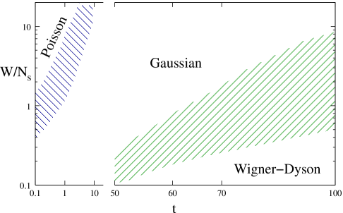
Figure 9: The statistics plot for the peak spacing for our dot model. We see rather broad crossover regions between the three asymptotic statistics. The region between Gaussian and Poisson in particular contains a broad parameter range where the distribution appears similar to a two-sided exponential.

We may summarize the results of the calculations as follows. In the classical limit with $t=0$ the effect of classical shells of charges on the CELS is small, even though the rearrangement of charges may be substantial.  Thus the width of $P(\Delta_{2})$ is dominated by the disorder even at quite small $W.$  This manifests itself as an increase in $\sigma,$ the width of $P(\Delta_{2})$ which is at first linear in $W$ (a finite-size effect) and then follows a square-root law. There is a crossover from pure Gaussian to a two-sided exponential-type function for $P(\Delta_{2})$ as $W$ increases. The crossover to a true Poisson distribution characteristic of strongly localized states occurs at much higher $W,$ probably outside the experimentally accessible range except for the most disordered samples. $\sigma$ is, however, very large in the classical case even for relatively modest values of $W.$  When quantum effects are turned on, the width of the distribution drops precipitously, owing to the usual level-repulsion effects. If the disorder is small, then the Gaussian $P(\Delta_{2})$ turns into the Wigner-Dyson form at about $r_{s}\sim 5-10.$  For larger disorder, the two-sided exponential distribution first turns into Gaussian and finally into Wigner-Dyson. This corresponds to the presence of classical disorder, interactions, and hopping, respectively. The new effect seen in our work is the two-sided exponential distribution. This appears because, unlike previous authors, we analyze the effect of strong disorder. In general, this effect is to modify the usual Gaussian distribution by first producing long tails, and then asymmetry in $P(\Delta_{2}).$

In Fig. 9, the results are summarized graphically in the statistics plot, as determined numerically. Although the numerical results are not definitive, they suggest that the phase boundaries between the various regions are more or less straight lines, and that there is always a Gaussian region that interposes between the Poisson and Wigner-Dyson regimes. Unfortunately, because of the surprisingly large crossover regions, we cannot completely resolve the topology of the plot.

5 Relation to Experiments

 

Figure 10: Fitting of the experimental data of Patel et al. (crosses) with Gaussian (dashed line) and two-sided exponential (solid line) functions. The two-sided exponential appears to be somewhat better fit.

Several experiments have been performed to measure the CELS. We discuss four of these.

The most detailed data come from the experiments of Patel et al. [15], who investigated seven GaAs quantum dots, all in the ballistic regime. Several thousand conductance peaks were examined, in contrast to the other reports, which contained of the order of one hundred. The mobilities ranged from ($1.4-6.5)$ $\times 10^{5}$ V-cm²/s, and the densities from $2-3\times 10^{11}/$cm${}^{2}.$  $r_{s}\approx 2-3$ for these samples.  $P(\Delta_{2})$ is very symmetric, but with very definite non-Gaussian tails. These data fit the two-sided exponential quite well, as seen in Fig. 10. The fit is not conclusive, but certainly suggests that there are tails induced by disorder in these samples. It is of particular interest that although the samples included have mobilities that vary by a factor of five, the fit with a single function is still satisfactory. This is probably due to the fact that the crossover region between Gaussian and Poisson statistics is almost vertical, as can be seen in Fig. 9.

In the experiment of Sivan et al. [5], the system was also a GaAs quantum dot, coming from a relatively high-mobility ($5\times 10^{5}$V-cm${}^{2}/$ s) sample with density $n_{s}=3.1\times 10^{11}/$ cm².  Thus the sample was very similar in terms of its disorder and density to those of Patel et al. $P(\Delta_{2})$ is again symmetric, but the statistics are insufficient to decide on whther the tails are non-Gaussian.

Other Coulomb blockade data come from Ref. [9], as extracted in Ref. [5]. This is a different system, consisting of In₂O_3-x wires that are insulating in the bulk. Unlike the quantum dots, these systems are believed to be well into the diffusive regime. There are relatively few accessible quantum states and the disorder is probably much stronger than in the other sample. There is some evidence of asymmetry in these data, a possible indication that this system belongs closer to the Poisson regime on the statistics plot, where the distribution becomes truly asymmetric.

Finally, we discuss the experiments of Simmel et al. [16].  These experiments were performed on a Si quantum dot. They are distinguished from the GaAs dots by a larger $r_{s}.$  We would expect the effects of disorder to be more pronounced. As in all the experiments except those of Patel et al., there are relatively few points, and it is therefore impossible to judge whether long tails are present. We note from Fig. 10 that asymmetry is much more likely to show up when $r_{s}$ increases ($t$ decreases in the figure). Given this, the suggestion of asymmetry in the data may indicate that the system is close to the Poisson crossover.

6 Conclusion

We have considered the effect of disorder and interactions on the CELS of quantum dots with a view towards obtaining a global picture of the CELS.  We computed the measurable quantity $P(\Delta_{2})$ numerically, averaging it over many realizations of the disorder. The chief new result is that strong disorder can modify the Gaussian statistics by producing first non-Gaussian tails and then asymmetry (skewness) in the distribution, leading ultimately to the Poisson distribution expected at very stroing disorder. These is good evidence for the tails and suggestions of the asymmetry, though relatively poor statistics makes it difficult to say that these effects have been unambiguously seen. We also find the expected crossover from Gaussian to Wigner-Dyson statistics as a function of $r_{s}.$  Our calculations, which include the long-range Coulomb interaction, suggest that the crossover occurs at somewhat larger $r_{s}$ than previous calculations on short-range models have given.

We thank S.N. Coppersmith, M.E. Eriksson, D.D. Long, and N.V. Lien for useful conversations and acknowledge the support of the National Science Foundation through Grant No. OISE-0435632, ITR-0325634, and the Army Research Office through Grant No. W911NF-04-1-0389.

References

- [1] For a detailed account of the history, see M.L. Mehta, Random Matrices, 2nd ed. (Academic Press, San Diego, 1991).
- [2] O. Bohigas, M.J. Giannoni and C. Schmit, Phys. Rev. Lett. 52, 1 (1984).
- [3] L. P. Gorkov and G. M. Eliashberg, Zh. Eksp. Teor. Fiz. 48, 1407 (1965); [Sov. Phys. JETP 21, 940 (1965)].
- [4] Y. Alhassid, Ph. Jacquod, and A. Wobst, Phys. Rev. B 61, R13357 (2000).
- [5] U. Sivan et al., Phys. Rev. Lett. 77, 1123 (1996).
- [6] A.J. Jalabert, A.D. Stone, and Y. Alhassid, Phys. Rev. Lett. 68, 3468 (1992); C.W.J. Beenakker, Rev. Mod. Phys. 69, 731 (1997).
- [7] A. Cohen, K. Richter, and R. Berkovits, Phys. Rev. B 60 2536 (1999).
- [8] C.M. Marcus, A.J. Rimberg, R.M. Westervelt, P.F. Hopkins, and A.C. Gossard, Microstructures”, Phys. Rev. Lett. 69 506 (1992).
- [9] V. Chandrasekhar and R. A. Webb, J. Low Temp. Phys. 97 , 9 (1994).
- [10] P. N. Walker, Y. Gefen, and G. Montambaux, Phys. Rev. Lett. 82, 5329 (1999).
- [11] B. I. Shklovskii, B. Shapiro,B. R. Sears, P. Lambrianides, and H. B. Shore, Phys. Rev. B 47, 11487 (1993).
- [12] R. Berkovits, Y. Gefen, I. V. Lerner, and B.L. Altshuler, Phys. Rev. B 68, 085314 (2003).
- [13] Y. Alhassid, H. A. Weidenmüller, and A. Wobs, Phys. Rev B 72, 045318 (2005).
- [14] A. A. Koulakov, F. G. Pikus, and B. I. Shklovskii, Phys. Rev. B 55, 9223 (1997); A. A. Koulakov and B. I. Shklovskii, Phys. Rev. B 57, 2352 (1998).
- [15] S. R. Patel, S. M. Cronenwett, D. R. Stewart, A. G. Huibers, and C. M. Marcus, Phys. Rev. Lett 80, 4522 (1998).
- [16] F. Simmel, D. Abusch-Magder, D. A. Wharam, M. A. Kastner, and J. P. Kotthaus, Phys. Rev. B 59, 10441 (1999).