Adiabatic Phase Diagram of an Ultracold Atomic Fermi Gas
with a Feshbach Resonance

Abstract

We determine the adiabatic phase diagram of a resonantly-coupled system of Fermi atoms and Bose molecules confined in the harmonic trap by using the local density approximation. The adiabatic phase diagram shows the fermionic condensate fraction composed of condensed molecules and Cooper pair atoms. The key idea of our work is conservation of entropy through the adiabatic process, extending the study of Williams et al. [Williams et al., New J. Phys. 6, 123 (2004)] for an ideal gas mixture to include the resonant interaction in a mean-field theory. We also calculate the molecular conversion efficiency as a function of initial temperature. Our work helps to understand recent experiments on the BCS-BEC crossover, in terms of the initial temperature measured before a sweep of the magnetic field.

1 Introduction

Degenerate Fermi gases with controllable interaction have been realized in recent experiments by making use of a Feshbach resonance. Much of the current study of these systems focuses on the crossover between a Bardeen-Cooper-Schrieffer (BCS) superfluid of fermionic atoms and Bose-Einstein condensation (BEC) of diatomic molecules [1, 2, 3, 4]. In these systems, the position of a molecular bound state can be tuned relative to the scattering continuum by varying an applied magnetic field. By ramping the magnetic field across a Feshbach resonance, one can continuously transform a fermionic atomic gas to a bosonic molecular gas, both above and below the superfluid transition temperature.

Several theoretical papers reported the phase diagrams of the resonantly-coupled Fermi-Bose mixture gas [5, 6, 7]. In order to compare these works with the experimental results by Regal et al. [1] and Zwierlein et al. [3], one has to understand how the system traverses the phase diagram as the resonance energy is varied. However, the experiments only provided a measure of the initial temperature, $T_{i}$, before the magnetic field sweep, thus complicating the attempts to relate the data to theoretical models. In the experiments, the sweep is slow so that atoms and molecules can move and collide sufficiently in the trap [3], allowing for relaxation to thermal and chemical equilibrium during the sweep. Assuming the sweep to be adiabatic , Williams et al. [8] calculated the phase diagram for the ideal gas mixture of fermionic atoms and bosonic molecules as a function of the resonance energy and $T_{i}$. The key idea of this adiabatic process is the conservation of entropy during the sweep: the system follows a path of constant entropy through the phase diagram, and the entropy is set by the initial preparation of the sample, i.e. the initial temperature. Using the reverse logic, Chen et al. [9] gave the idea of thermometry, by which the real temperature of the system after an adiabatic sweep may be deducted from the initial temperature before the sweep. Based on this finite temperature formalism, they compared the experimental phase diagram with their theoretical boundary between the normal phase and the superfluid phase [10]. Similar ideas were proposed by Hu et al. [11] and Carr et al. [12].

In this paper, we extend the work by Williams et al. [8] for an ideal gas mixture of fermionic atoms and bosonic molecules to include the resonant interaction using mean-field theory. Our mean-field treatment allows for the description of the BCS superfluidity due to the interaction, which was neglected in ref. 8. In order to introduce the effect of the harmonic trap, we apply the local density approximation (LDA).

Calculating the entropy as a function of the temperature and the detuning, we show the paths of constant entropy traversed in the conventional phase diagrams as the detuning is varied adiabatically. On the basis of the adiabatic path, we determine the adiabatic phase diagrams against the detuning and entropy, labeled by the initial temperature of the Fermi gas measured before a sweep of the magnetic field. We note that the adiabatic phase diagram of ref. 10 plots the superfluid fraction, whose phase boundary has a good agreement with the experiment in ref. 1, while the experimental phase diagrams [1, 3] show the condensate fraction which is zero momentum molecules projected through the fast sweep, assuming that the fraction has an information of zero momentum molecules and zero center-of-mass momentum Cooper pairs. In this paper, we plot the phase diagrams for the condensate fraction that is composed of zero momentum molecules and zero momentum Cooper pairs.

We are also interested in the production efficiency of molecules during the adiabatic sweep of the magnetic field. The conversion efficiency is found experimentally to be a monotonic function of the initial peak phase space density, when the magnetic field is swept adiabatically [13]. A recent paper by Williams et al. [14] discussed the mechanism of molecular formation, in the case where three-body recombination may be neglected, and derived an expression for the molecular conversion efficiency in terms of the initial peak phase-space density. Their result agrees with the experimental data [13] although they treat a non-interacting quantum gas. We extend the calculation of the molecular conversion efficiency in ref. 14 to include the mean-field effect.

Our study gives an intuitive understanding of recent experiments on the BCS-BEC crossover using the adiabatic sweep process.

2 Equilibrium Theory

Our model is the coupled boson-fermion Hamiltonian with a two-component Fermi gas [6, 15, 16];

$$\hat{H} = \int d{\bf r}[\hat{\psi}^{{\dagger}}_{\sigma}({\bf r})H_{a}({\bf r})\hat{\psi}_{\sigma}({\bf r})+\hat{\phi}^{{\dagger}}({\bf r})H_{m}({\bf r})\hat{\phi}({\bf r})]$$ (1)

$$+\kappa\int d{\bf r}[\hat{\phi}^{{\dagger}}({\bf r})\hat{\psi}_{\uparrow}({\bf r})\hat{\psi}_{\downarrow}({\bf r})+\hat{\psi}^{{\dagger}}_{\downarrow}({\bf r})\hat{\psi}^{{\dagger}}_{\uparrow}({\bf r})\hat{\phi}({\bf r})],$$

where repeated indices $\sigma$ imply a sum over pseudospin states $\sigma=\{\uparrow,\downarrow\}$. The field operators of atoms and molecules are respectively denoted as $\hat{\psi}_{\sigma}({\bf r})$ and $\hat{\phi}({\bf r})$, which obey Fermi and Bose commutation relations. The single particle Hamiltonians for the atoms and molecules are given by $H_{a}({\bf r})=-(\hbar^{2}/2m)\nabla^{2}+V_{a}({\bf r})$ and $H_{m}({\bf r})=-(\hbar^{2}/2M)\nabla^{2}+V_{m}({\bf r})+\delta$ , respectively, where $m$ is the atomic mass and $M=2m$ is the molecular mass. We introduce the harmonic trap in which the each pseudo-spin Fermi atoms feel the same potential, given by $V_{a}({\bf r})=m\omega_{0}^{2}r^{2}/2$. On the other hand, we assume that molecules feel the following potential: $V_{m}({\bf r})=M\omega_{0}^{2}r^{2}/2$. This assumption is valid for the current experiments in optical dipole traps [17]. Two fermionic atoms are coupled to a bosonic molecule through the resonant interaction with the coupling constant $\kappa$. The detuning $\delta(B)$ can be tuned by adjusting an external magnetic field $B$, since the bare atoms and molecules have different magnetic moments, and thus experience a relative linear Zeeman shift. As usual we take the zero of energy to be the energy of two separated atoms at rest at each value of $B$. We neglect the non-resonant atom-atom interaction, since the effective interaction for two atoms is dominated by the resonant contribution $-\kappa^{2}/\delta$ near the resonance.

In order to impose the constraint that the number of particles be conserved, we introduce the chemical potential and deal with the grand canonical Hamiltonian $\hat{{\mathcal{H}}}\equiv\hat{H}-\mu\hat{N}$, where the total number operator of particles is defined as $\hat{N}\equiv\int d{\bf r}[\sum\limits_{\sigma}\hat{\psi}^{{\dagger}}_{\sigma}({\bf r})\hat{\psi}_{\sigma}({\bf r})+2\hat{\phi}^{{\dagger}}({\bf r})\hat{\phi}({\bf r})]$. The factor of two in the last term reflects that each molecules are assembled from two atoms. We regard the system as in chemical equilibrium between atoms and molecules [8, 18].

In the superfluid phase, we can separate the molecular field operator into two parts:

$$\hat{\phi}({\bf r}) = \langle\hat{\phi}({\bf r})\rangle+\tilde{\phi}({\bf r})$$ (2)

$$= \Phi({\bf r})+\tilde{\phi}({\bf r}).$$

Here, $\Phi({\bf r})$ represents the molecular condensate wavefunction, which corresponds to the order parameter, and $\tilde{\phi}({\bf r})$ represents the non-condensate molecules. In the mean-field theory, one leaves out the Cooper pairs outside the condensate, and the Hamiltonian $\hat{\mathcal{H}}$ reduces to the BCS-type Hamiltonian [15]

$$\hat{\mathcal{H}} = \int d{\bf r}\{\Phi^{*}({\bf r})[H_{m}({\bf r})-2\mu]\Phi({\bf r})\}+\int d{\bf r}\{\tilde{\phi}^{\dagger}({\bf r})[H_{m}({\bf r})-2\mu]\tilde{\phi}({\bf r})\}$$

$$+\int d{\bf r}\{\hat{\psi}^{{\dagger}}_{\sigma}({\bf r})[H_{a}({\bf r})-\mu]\hat{\psi}_{\sigma}({\bf r})\}+\kappa\int d{\bf r}[\Phi^{*}({\bf r})\hat{\psi}_{\uparrow}({\bf r})\hat{\psi}_{\downarrow}({\bf r})+\hat{\psi}^{{\dagger}}_{\downarrow}({\bf r})\hat{\psi}^{{\dagger}}_{\uparrow}({\bf r})\Phi({\bf r})],$$

where fluctuation terms like $\tilde{\phi}^{\dagger}\hat{\psi}_{\downarrow}\hat{\psi}_{\uparrow}$ have been neglected.

This type of quadratic Hamiltonian can be diagonalized by the standard Bogoliubov transformation. In order to discuss the thermodynamics of the system, we evaluate the grand canonical potential $\Omega$. The effect of a harmonic trap in the grand canonical potential $\Omega$ is included by the local density approximation [5], which adopts the effect of the local potential by replacing the chemical potential $\mu$ with $\mu({\bf r})=\mu-V_{a}({\bf r})$.

The grand canonical potential including the effect of the harmonic trap potential is given by

$$\Omega = \int d{\bf r}\left([\delta-2\mu({\bf r})]|\Phi({\bf r})|^{2}+\frac{1}{\beta}\int\frac{d{\bf k}}{(2\pi^{3})}\ln{\{1-e^{-\beta[\varepsilon_{\bf k}^{(m)}+\delta-2\mu({\bf r})]}\}}\right.$$ (5)

$$+\left.\int\frac{d{\bf k}}{(2\pi^{3})}\left\{[\varepsilon_{\bf k}^{(a)}-\mu({\bf r})-E_{\bf k}({\bf r})]-\frac{2}{\beta}\ln{[1+e^{-\beta E_{\bf k}({\bf r})}]}\right\}\right).$$

Here, $\varepsilon^{\scriptsize{(m)}}_{{\bf k}}=\hbar^{2}{\bf k}^{2}/2M$ is the kinetic energy of a molecule, and $\varepsilon^{\scriptsize{(a)}}_{{\bf k}}=\hbar^{2}{\bf k}^{2}/2m$ is the kinetic energy of an atom. As usual $\beta=1/kT$, where $T$ is the temperature and $k$ is Boltzmann’s constant. At this step, we have already assumed that the atoms and molecules are in thermal equilibrium. In other words, the atom temperature and the molecule temperature are the same [8, 18]. The local quasiparticle excitation energy is $E_{{\bf k}}({\bf r})=\sqrt{[\varepsilon_{{\bf k}}^{(a)}-\mu({\bf r})]^{2}+|\Delta({\bf r})|^{2}}$, where the local gap energy is $|\Delta({\bf r})|=\kappa|\Phi({\bf r})|$. Within our mean-field theory, the excitation spectrum of bosonic molecules has the finite excitation gap $\delta-2\mu$. However, in the superfluid phase, the symmetry breaking requires a gapless spectrum with the Bogoliubov phonon mode. This can be incorporated into the theory by including the effect of fluctuations [19], which are neglected in our mean-field theory. The gapless excitations are important at very low temperatures. We will discuss this point in § 3.

The local gap equation is obtained from $\delta\Omega/\delta|\Phi({\bf r})|=0$ , which leads to

$$\delta-2\mu({\bf r})=\frac{\kappa^{2}}{2}\int\frac{d{\bf k}}{(2\pi)^{3}}\frac{1}{E_{{\bf k}}({\bf r})}\tanh{\left[\frac{\beta E_{{\bf k}}({\bf r})}{2}\right]}.$$ (6)

On the other hand, the total number of particles $N_{\rm{tot}}$ follows from the relation $N_{\rm{tot}}=-\partial\Omega/\partial\mu$, which gives

$$N_{\rm{tot}} = 2\int d{\bf r}|\Phi({\bf r})|^{2}+2\int\frac{d{\bf r}d{\bf k}}{(2\pi)^{3}}f_{B}(\varepsilon_{{\bf k}}^{{\scriptsize{(m)}}};{\bf r})$$ (7)

$$+\int\frac{d{\bf r}d{\bf k}}{(2\pi)^{3}}\left[1-\frac{\varepsilon_{{\bf k}}^{{\scriptsize{(a)}}}-\mu({\bf r})}{E_{{\bf k}}({\bf r})}+2\frac{\varepsilon_{{\bf k}}^{{\scriptsize{(a)}}}-\mu({\bf r})}{E_{{\bf k}}({\bf r})}f_{F}(E_{{\bf k}};{\bf r})\right].$$

Here, the Bose and Fermi local distribution functions are respectively $f_{B}(\varepsilon_{{\bf k}}^{\scriptsize{(m)}};{\bf r})$ and $f_{F}(E_{{\bf k}};{\bf r})$, which are given by $f_{B}(\varepsilon_{{\bf k}}^{\scriptsize{(m)}};{\bf r})=1/\{\exp{[\beta(\varepsilon_{{\bf k}}^{\scriptsize{(m)}}+\delta-2\mu({\bf r}))]}-1\}$ and $f_{F}(E_{{\bf k}};{\bf r})=1/[\exp{(\beta E_{{\bf k}}({\bf r}))}+1]$ . In the right-hand-side of eq. (7), the first term represents the twice number of the condensed molecules $2N_{mc}$. The second term represents the twice number of the non-condensed molecules $2\tilde{N}_{m}$. The last term is the number of atoms $N_{a}$. Thus, eq. (7) can be written as

$$N_{\rm tot} = 2N_{m}+N_{a}$$ (8)

$$= 2N_{mc}+2\tilde{N}_{m}+N_{a}.$$

We also calculate the condensed pair number $N_{c}$, which is composed of the number of condensed molecules $N_{mc}$ and Cooper pairs $N_{p}$:

$$N_{c} = N_{mc}+N_{p}$$ (9)

$$= \int d{\bf r}|\Phi({\bf r})|^{2}+\int d{\bf r}_{1}d{\bf r}_{2}|\langle\hat{\Psi}_{\uparrow}({\bf r}_{1})\hat{\Psi}_{\downarrow}({\bf r}_{2})\rangle|^{2},$$

where the second term of eq. (9) describing the number of the condensed Cooper pair is the maximum eigenvalue of two-particle density matrix [20]. Within our mean-field theory, the explicit expression for the number of Cooper pairs $N_{p}$ is given by [21, 22]

$$N_{p} = \int\frac{d{\bf r}d{\bf k}}{(2\pi)^{3}}\left\{\frac{|\Delta({\bf r})|^{2}}{4E^{2}_{{\bf k}}({\bf r})}\tanh^{2}{\left[\frac{\beta E_{{\bf k}}({\bf r})}{2}\right]}\right\}.$$ (10)

We regard eqs. (6) and (7) as the simultaneous equations for the chemical potential $\mu$ and the local gap $|\Delta({\bf r})|$, for a given temperature $T$ and detuning $\delta$. In this paper, we set the bare coupling strength to $\alpha\equiv\sqrt{\rho}\kappa=0.4\varepsilon_{\rm F}$, where $\rho$ is the peak density and $\varepsilon_{\rm F}$ is the Fermi energy of a pure gas of fermionic atoms, which corresponds to the narrow Feshbach resonance, which is given by $\rho=(2m\varepsilon_{\rm F})^{\frac{3}{2}}/(3\pi^{2}\hbar^{3})$ and $\varepsilon_{\rm F}=(3N_{\rm tot})^{\frac{1}{3}}\hbar\omega_{0}$. This weak coupling constant allows for a mean-field treatment. Although this value does not correspond to experimental situation of the broad Feshbach resonance, discussed in ref. 23 (see also discussion in § 3), we do not expect any qualitative differences in equilibrium phase diagrams between narrow and broad Feshbach resonances. To avoid the divergence of the integral in eq. (6), we impose the Gaussian cut-off; $\exp{\{-[\varepsilon/(2\varepsilon_{\rm F})]^{2}\}}$, whose cutoff energy scale is chosen to be the Fermi energy [5].

3 Adiabatic Phase Diagram

In this section, we discuss the adiabatic phase diagram. We first briefly review the experimental procedures of refs. 1 and 3. In these experiments, the ultracold two-component Fermi gas is initially prepared at a magnetic field far detuned from the resonance position, corresponding to a pure atomic gas. In this weakly interacting regime the temperature of the Fermi gas is measured using time-of-flight imaging. The magnetic field is then slowly lowered to the vicinity of the resonance to allow the atoms and molecules sufficient time to move and collide in the trap. This process may satisfy the condition that the gas be able to collisionally relax to equilibrium [8]. We regard this process as an adiabatic quasistatic process, because the magnetic field is varied while keeping the thermal and chemical equilibrium from moment to moment without exchanging heat or particles with the environment. The system will thus follow a path of constant entropy in the phase diagram.

The total entropy $S_{\rm tot}$ is the sum of the atom entropy $S_{a}$ and the molecule entropy $S_{m}$. These are given by

$$S_{a} = 2k_{B}\int\frac{d{\bf r}d{\bf k}}{(2\pi)^{3}}\left\{\frac{\beta E_{{\bf k}}({\bf r})}{e^{\beta E_{{\bf k}}({\bf r})}+1}+\ln{[1+e^{-\beta E_{{\bf k}}({\bf r})}]}\right\},$$ (11)

and

$$S_{m} = k_{B}\int\frac{d{\bf r}d{\bf k}}{(2\pi)^{3}}\left(\frac{\beta[\varepsilon_{{\bf k}}^{\scriptsize{(M)}}+\delta-2\mu({\bf r})]}{e^{\beta[\varepsilon_{{\bf k}}^{\scriptsize{(M)}}+\delta-2\mu({\bf r})]}-1}-\ln{\{1-e^{-\beta[\varepsilon_{{\bf k}}^{\scriptsize{(M)}}+\delta-2\mu({\bf r})]}\}}\right).$$ (12)

Before showing contours of constant entropy, we plot the conventional phase diagrams of the condensed molecular fraction $\eta_{mc}=2N_{mc}/N_{\rm tot}$ and the condensed Cooper pair fraction $\eta_{p}=2N_{p}/N_{\rm tot}$ separately against the temperature $T$ and the detuning $\delta$ in Figs. 1 (A) and 1 (B). From Fig. 1 (B), we find that the number of Cooper pairs at low temperatures is peaked above the resonance in the BCS regime, while its contribution to the total condensed fraction $\eta_{c}$ is very small. This is because we deal with the weak coupling (narrow Feshbach resonance). In the case of the strong coupling (broad Feshbach resonance), the Cooper pair contribution in the fermionic condensate fraction becomes dominant, and the single channel model describes effectively such systems in the vicinity of the resonance [24]. However, as shown in ref. 23, the conventional phase diagrams are almost the same for both cases, when plotted against $(k_{\rm F}a_{s})^{-1}$ instead of $\delta$ ($k_{\rm F}$ is the Fermi wavenumber and $a_{s}$ is the $s$-wave scattering length). ref. 23 also shows that the behaviors of the total number of bosons (including both Cooper pairs in the open channel and bare molecules of the closed channel) are almost the same for the two cases. We thus expect that the adiabatic phase diagram discussed below also describes the qualitative behavior in the broad resonance case.

Figure 1: (Color online) (A) Conventional phase diagram of the condensed molecular fraction $\eta_{mc}$. (B) Conventional phase diagram of the condensed Cooper pair fraction $\eta_{p}$. Note the change in colorscale between panels (A) and (B). Each fraction in the conventional phase diagram is plotted against the temperature $T$ and the detuning $\delta$, normalized by the Fermi energy. (C) Contours of constant entropy. The paths are plotted against the temperature $T$ and the detuning $\delta$, as the detuning is varied adiabatically. We set the coupling strength $\alpha=0.4\varepsilon_{\rm F}$.

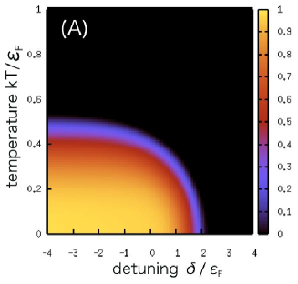
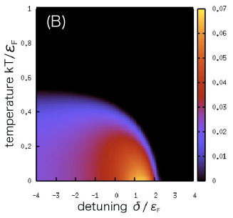
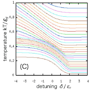
In Fig. 1 (C), we show contours of constant entropy in the $\delta$ - $T$ plane. We recognize those lines, as the paths that are traversed as the detuning $\delta$ is swept adiabatically, starting from the right side of the resonance at a large value of the detuning $\delta$. We see that the temperature increases as the detuning $\delta$ is lowered adiabatically. This temperature increase on the path of constant entropy can be understood as follows: first, due to the conversion of pairs of atoms into molecules, the system loses degrees of freedom; second, the condensed molecules does not contribute to the entropy; third, the existence of Cooper pairs also suppresses the entropy. For these reasons, the system must then heat up in order to conserve the entropy.

The relation between the initial temperature of the atomic gas and the final temperature of the molecular gas has been given for the ideal gas mixture of fermionic atoms and bosonic molecules by Williams et al. [8]. In the low-temperature limit $T/T_{\rm F}\ll 1$, one finds

$$\frac{T_{f}}{T_{\rm F}}=\left[\frac{\pi^{2}}{12\zeta(4)}\right]^{1/3}\left(\frac{T_{i}}{T_{\rm F}}\right)^{1/3},$$ (13)

while in the high-temperature limit, $T/T_{\rm F}\gg 1$, the relation becomes

$$\frac{T_{f}}{T_{\rm F}}=6^{1/3}{\rm e}^{4/3}\left(\frac{T_{i}}{T_{\rm F}}\right)^{2}.$$ (14)

The above relations can be derived by connecting the initial entropy of a pure atomic gas and the final entropy of a pure molecular gas. Similar expressions have been derived by Carr et al. [25] in connection with the idea of cooling a Fermi gas by adiabatically increasing the magnetic field starting from a molecular gas.

Figure 2: The final temperature versus the initial temperature where the final detuning is $\delta/\varepsilon_{\rm F}=-100$ (solid line) and $\delta/\varepsilon_{\rm F}=-4$ (dotted line). The dashed and dot-dashed lines represent the high and low temperature limit. We set the coupling strength $\alpha=0.4\varepsilon_{\rm F}$.

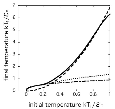
In Fig. 2, we plot the final temperature in a deeply BEC region and a moderately BEC region as a function of the initial temperature. The solid line is obtained by a numerical calculation in a deeply BEC region where the detuning is $\delta=-100\varepsilon_{\rm F}$. The dotted line is obtained by a numerical calculation in a moderately BEC region where the detuning is $\delta=-4\varepsilon_{\rm F}$. The dashed line represents the high-temperature limit for an ideal gas, while the dot-dashed line represents the low-temperature limit for an ideal gas. The low-temperature approximation agrees with the both of numerical solutions. The high temperature approximation does not agree with the numerical solution of a moderately BEC region, because atoms appear when the temperature is not sufficiently high and the concept of connecting the entropy of a pure atomic gas and that of a gas consisting entirely of molecules breaks down. On the other hand, the high temperature approximation agrees with a numerical solution of a deeply BEC region except for the high initial temperature regime where some atoms remain at the end of the sweep. These agreements are reasonable since our model assumes the narrow resonance case, leaving out the Cooper pairs outside the condensate. The system is equivalent to the ideal gas mixture for temperatures above $T_{c}$.

Figure 3: (Color online) The adiabatic phase diagram. The total fermionic condensate fraction $\eta_{c}=\eta_{mc}+\eta_{p}$ is plotted against the initial temperature $T_{\rm i}$ and the detuning $\delta$.

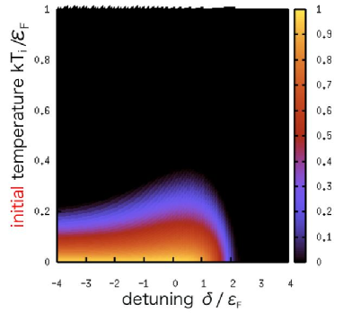
In Fig. 3, we plot the fermionic condensate fraction $\eta_{c}=2N_{c}/N_{\rm tot}$ against the detuning $\delta$ and the initial temperature of the atomic Fermi gas measured before a sweep of the magnetic field, as in the experimental phase diagrams of refs. 1 and 3. The initial temperature $T_{i}$ is found by equating the total entropy to the initial entropy $S_{\rm tot}(\delta,T)=S_{i}(T_{i})$.

In Figs. 1 (A) and 1 (B), the transition temperature is $T_{c}\simeq 0.53T_{\rm F}$ in the BEC region where the detuning is $\delta=-4\varepsilon_{\rm F}$. On the other hand, in Fig. 3, the transition temperature in terms of the initial temerature is $T_{i,c}\simeq 0.21T_{\rm F}$ at $\delta=-4\varepsilon_{\rm F}$. This behavior is consistent with Williams et al. [8] for an ideal gas model, where the transition temperature is $T_{c}\simeq 0.51T_{\rm F}$ and the transition temperature in terms of the initial temerature is $T_{i,c}\simeq 0.21T_{\rm F}$ at $\delta=-4\varepsilon_{\rm F}$. The difference in the transition temperature between our model and the ideal gas model becomes smaller when we translate the conventional transition temperature to the transition temperature in terms of the initial temperature. This translated transition temperature $T_{i,c}$ in the BEC limit is comparable with transition temperature observed in the experiments [1, 3]. Here we comment on the finite energy gap of bosonic excitations discussed in § 2. Because of this artificial gap, our mean-field results should be unreliable in the low temperature region where $k_{B}T<\delta-2\mu$. However in our adiabatic phase diagram, for $\delta<0.5\varepsilon_{\rm F}$, the real temperature satisfies the inequality $k_{B}T\gg\delta-2\mu$ as long as the initial temperature satisfies $k_{B}T_{i}>0.05\varepsilon_{\rm F}$. The region where the real temperature satisfies $k_{B}T\gg\delta-2\mu$ becomes wider as one goes into the BEC side of the resonance. On the other hand, for $\delta>0.5\varepsilon_{\rm F}$, the total number of molecules is so small at low temperatures, that the bosonic excitations make no significant contribution to the thermodynamic. Therefore, the finite energy gap in the bosonic excitation spectrum due to the mean-field treatment does not affect our adiabatic phase diagram significantly except for the low temperature region $k_{B}T_{i}<0.05\varepsilon_{\rm F}$ in the crossover region $\delta\sim 0$.

Figure 4: (Color online) The fermionic condensate fraction $\eta_{c}$, the condensed molecular fraction $\eta_{mc}$ and the molecular fraction $\eta_{m}$ for the initial temperature $T_{\rm i}=0.08T_{\rm F}$ are plotted against the detuning $\delta$. The solid line represents the fermionic condensate fraction $\eta_{c}$. The dotted line represents the condensed molecular fraction $\eta_{mc}$. The dashed line represents the molecular fraction $\eta_{m}$. We set the coupling strength $\alpha=0.4\varepsilon_{\rm F}$.

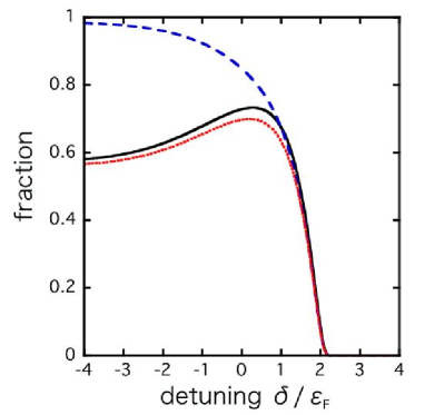
In Fig. 4, we plot the fermionic condensate, the condensed molecular, and the total molecular fractions with an initial temperature $T_{i}/T_{\rm F}=0.08$ as a function of the detuning. As the detuning is lowered, the fermionic condensate fraction increases. Subsequently it decreases after having a peak near the resonance. This behavior is consistent with experiments [1, 3]. Williams et al. [8] finds a similar result for an ideal gas mixture, though they normalize the condensate fraction by the number of molecules.

4 Molecular Conversion Efficiency

Hodby et al. [13] have investigated the molecular conversion efficiency in bosonic ⁸⁵Rb and fermionic ⁴⁰K. They found that the molecular conversion efficiency does not reach 100% even for an adiabatic sweep, but saturates at a value, that depends on initial peak phase-space density. Their experimental data is simulated by a Monte Carlo-type simulation [13] based on a model assuming that pairing formation occurs when two atoms are close enough in the phase space.

On the other hand, Williams et al. [14] discussed the molecular conversion efficiency assuming the molecular formation rate vanishes when the detuning $\delta$ is negative. Their result is derived by using the coupled atom-molecule Boltzmann equations. They calculated the conversion efficiency from the molecular fraction at the detuning $\delta=0$ as a function of the initial peak phase space density, and found good agreement with the experimental data although they treated an ideal gas mixture of Fermi atoms and Bose molecules. We note that the initial temperature and the initial phase space density have a one-to-one correspondence.

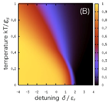
In the experiment for ⁴⁰K, the conversion fraction does not depend on the inverse sweep rate within a range from $640$ to $2900\mu s/G$. In this range, therefore the conversion process can be considered as adiabatic [13]. According to the kinetic theory of ref. 18, in this regime the chemical equilibration between atoms and molecules also brings about the thermal equilibration. Assuming this adiabatic limit and that the principle controlling the maximum molecular conversion efficiency proposed by Williams et al. also applies when including the resonant interaction, we calculate the molecular conversion efficiency using $\eta_{m}(\delta=0)$ as a function of initial temperature, as shown in Fig. 5 (A), where $\eta_{m}$ is the molecular fraction $2N_{m}/N_{\rm tot}$. We note that the Feshbach resonance of ⁴⁰K is known to be broad [13]. Although our mean-field theory is only applicable to the narrow resonance case, we can see the qualitative effect of the resonance interaction from Fig. 5 (A). The dotted line represents the result from our model, while the dot-dashed line represents the ideal gas mixture of Fermi atoms and Bose molecules [14]. The dots represent the data of Hodby et al. [13], and the solid line represents their simulation result. Dashed lines represent the uncertainty of the pairing parameter in their simulation. As noted above, the weak coupling constant we used does not directly correspond to the experiment, and thus the comparison between the theory and experiment is only qualitative. Nevertheless we find that our model agrees well with the trend of experimental data. The transition temperature $T_{c}$ at $\delta=0$ is $0.45T_{\rm F}$, which corresponds to the transition temperature in terms of initial temperature $T_{i,c}=0.36T_{\rm F}$. Above $T_{i,c}$ our model is identical to the ideal gas mixture case, since we are treating the resonant interaction in a mean-field theory. For reference, we show the molecular fraction $\eta_{m}$ plotted as a function of temperature and the detuning in Fig. 5 (B). The fraction at the resonance position $\delta=0$ and a temperature adiabatically connected with the initial temperature are used for the conversion efficiency in Fig. 5 (A).

Figure 5: (Color online) (A) The molecular conversion efficiencies are plotted against the initial temperature. The dotted line represents the our model, while the dot-dashed line is the result for an ideal gas mixture [14]. The dots represent the experimental data of Hodby et al. [13]. The solid line represents their simulation result, and the dashed lines give the uncertainty of the pairing parameter in their simulation. (B) For reference, the molecular fraction $\eta_{m}$ is plotted as a function of temperature and the detuning. The fraction at the resonance position $\delta=0$ and a temperature adiabatically connected with the initial temperature are used for the conversion efficiency in Fig. (A). We set the coupling strength $\alpha=0.4\varepsilon_{\rm F}$.

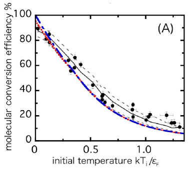
The resonant interaction is more important for lower initial temperatures. At the initial temperature $T_{i}=0$, the molecular conversion efficiency is 100% in the ideal gas mixture model. On the other hand, the experimental data at $T_{i}\rightarrow 0$ is suppressed from 100%. The efficiency in our model at $T_{i}=0$ is also less than 100%, because the resonant interaction suppresses the molecular conversion. We note that the resonance position may shift from the ideal gas case due to the atom-molecule interaction, which may also shift the result for the conversion efficiency quantitatively. However, the qualitative relation between the molecule conversion efficiency and the initial temperature will remain unchanged.

5 Conclusion

In this paper, we have calculated the phase diagrams for resonantly-coupled system of Fermi atoms and Bose molecules. We determined the paths of constant entropy traversed in the phase diagram as the detuning is lowered adiabatically. The adiabatic phase diagram of the fermionic condensate fraction composed of the condensed molecules and the Cooper pairs was plotted against the detuning $\delta$ and the initial temperature of a pure atomic gas. The adiabatic phase diagram allowed us to compare the theory with experiments, since in the experients [1, 3], the condensate fraction have been measured against the initial temperature and the magnetic field. We obtained the transition temperature in terms of the initial temperature $T_{i,c}\simeq 0.21T_{\rm F}$ in the BEC regime. Finally, the molecular conversion efficiency was plotted as a function of the initial temperature. We found that the resonant interaction suppresses the complete conversion.

The present work is an extension of the recent works by Williams et al. [8, 14] to include the resonant interaction using a mean-field theory. Although our model assumes a narrow resonance, the mean-field calculations help qualitative understanding of the recent experiments on the BCS-BEC crossover. In particular, the suppression of $T_{i,c}$ in the BEC limit and the behavior of the molecular conversion efficiency will be qualitatively unchanged even in the broad resonance case. In order to compare the theory with experiments in a quantitative fashion, we must include the Cooper pairs outside the condensate, which are neglected in our mean-field calculation. We must also express the resonance position in terms of the magnetic field rather than the detuning.

6 Acknowledgements

We thank Chikara Ishii and Satoru Konabe for helpful discussions and continuous encouragements. We also thank Allan Griffin for useful comments.

References

- [1] C. A. Regal, M. Greiner, and D. S. Jin, Phys. Rev. Lett. 92 (2004) 040403.
- [2] M. Bartenstein, A. Altmeyer, S. Riedl, S. Jochim, C. Chin, J. Hecker Denschlag, and R. Grimm, Phys. Rev. Lett. 92 (2004) 120401.
- [3] M. W. Zwierlein, C. A. Stan, C. H. Schunck, S. M. Raupach, A. J. Kerman, and W. Ketterle, Phys. Rev. Lett. 92 (2004) 120403.
- [4] T. Bourdel, L. Khaykovich, J. Cubizolles, J. Zhang, F. Chevy, M. Teichmann, L. Tarruell, S. J. J. M. F. Kokkelmans, and C. Salomon, Phys. Rev. Lett. 93 (2004) 050401.
- [5] Y. Ohashi, and A. Griffin, Phys. Rev. A 67 (2003) 033603.
- [6] G. M. Falco, and H. T. C. Stoof, Phys. Rev. Lett. 92 (2004) 130401.
- [7] R. B. Diener, and T. - L. Ho, cond-mat / 0404517.
- [8] J. E. Williams, N. Nygaard, and C. W. Clark, New J. Phys. 6 (2004) 123.
- [9] Q. Chen, J. Stajic, and K. Levin, Phys. Rev. Lett. 95 (2005) 260405.
- [10] Q. Chen, C. A. Regal, M. Greiner, D. S. Jin, and K. Levin, Phys. Rev. A 73 (2006) 041601.
- [11] H. Hu, X.-J. Liu, and P. Drummond, Phys. Rev. A 73 (2006) 023617.
- [12] L. D. Carr, R. Chiaramonte, and M. J. Holland, Phys. Rev. A 70 (2006) 043609.
- [13] E. Hodby, S. T. Thompson, C. A. Regal, M. Greiner, A. C. Wilson, D. S. Jin, E. A. Cornell, and C. E. Wieman, Phys. Rev. Lett. 94 (2005) 120402.
- [14] J. E. Williams, N. Nygaard, and C. W. Clark, New J. Phys. 8 (2006) 150.
- [15] Matt Mackie, and Jyrki Piilo, Phys. Rev. Lett. 94 (2005) 060403.
- [16] Y. Kawaguchi, and T. Ohmi, cond-mat / 0411018.
- [17] M. W. Zwierlein, C. A. Stan, C. H. Schunck, S. M. F. Raupach, S. Gupta, Z. Hadzibabic, and W. Ketterle, Phys. Rev. Lett. 91 (2003) 250401.
- [18] J. E. Williams, T. Nikuni, N. Nygaard, and C. W. Clark, J. Phys. B: At. Mol. Opt. Phys. 37 (2004) L351.
- [19] Y. Ohashi, and A. Griffin, Phys. Rev. A 67 (2003) 063612.
- [20] C. N. Yang, Rev. Mod. Phys. 34 (1962) 694.
- [21] M. H. Szymańska, K. Góral, T. Köhler, and K. Burnett, Phys. Rev. A 72 (2005) 013610.
- [22] L. Salasnich, N. Manini, and A. Parola, Phys. Rev. A 72 (2005) 023621.
- [23] Y. Ohashi, and A. Griffin, Phys. Rev. A 72 (2005) 013601.
- [24] Y. Ohashi, and A. Griffin, Phys. Rev. A 72 (2005) 063606.
- [25] L. D. Carr, G. V. Shlyapnikov, and Y. Castin, Phys. Rev. Lett. 92 (2004) 150404.