Multifractal fluctuations in the survival probability of an open quantum system

Abstract

We predict a multifractal behaviour of transport in the deep quantum regime for the opened $\delta-$kicked rotor model. Our analysis focuses on intermediate and large scale correlations in the transport signal and generalizes previously found parametric mono-fractal fluctuations in the quantum survival probability on small scales.

I Introduction

Multifractal analysis of fluctuating signals is a widely applied method to characterize complexity on many scales in classical dynamics Ott1993 , or in the analysis of a given time series (without any a priori knowledge on the underlying dynamical system which generated the series) Kantz .

On the quantum level, multifractal behaviour was found in the scaling of eigenfunctions in solid-state transport problems Qmulti . As far as we know, there have been, however, very few attempts to use the method of multifractal analysis to directly characterize transport properties such as conductance (across a solid state sample) or the survival probability (in open, decaying systems). Often it is indirectly argued that the multifractal structure of the wave functions at critical points (at the crossover between the localized and the extended regime) imprints itself on the scaling of transport coefficients SM2005 . Other works found a fractal scaling of local transport quantities, such as hopping amplitudes BKAHB2001 or two-point correlations JMZ1999 . At criticality JMZ1999 predicts, e.g., a multifractal scaling of the two-point conductance between two small interior probes within the transporting sample.

In this paper, we directly study the fluctuations properties of a global conductance like quantity in a regime of strong localization (Anderson or dynamical localization in our context of quantum dynamical systems). The studied quantity is the survival probability of an open, classically chaotic system, which in the deep quantum realm was found to obey a monofractal scaling if certain conditions on the quantum eigenvalue spectrum are fulfilled GT2001 ; TMW2006 . In particular, the distribution of decay rates of the weakly opened system needs to obey a power-law with an exponent $\gamma\sim-1$, which translates into an analytic prediction for the corresponding box counting dimension (of the survival probability as a function of a proper scan parameter): $D_{\rm BC}\simeq 2-|\gamma|/2$.

A more detailed, yet preliminary numerical analysis of the decay rate distribution for our model system (to be introduced below) has found that two scaling regions can be identified T2001 . While for small rates the probability density function $\rho(\Gamma)$ scales as $\Gamma^{-1}$, at larger scales it turns to $\Gamma^{-3/2}$ – which is expected for strongly transmitting channels from various models for transport through disordered systems BGS1991 . Here we ask ourselves whether this prediction of a smooth variation in the scaling of the monofractal behaviour (induced by the smoothly changing exponent $\gamma$) can be generalized to characterize the fluctuations on many scales using from the very beginning the technique of multifractal analysis. Before we present our findings on the multifractal scaling of the parametric fluctuations of the survival probability, we introduce the kicked rotor system and our numerical algorithm for the multifractal analysis in the subsequent two sections.

II Our transport model and the central observable

The $\delta-$kicked rotor is a widely studied, paradigmatic toy model of classical and quantum dynamical theory Chi1979 ; Izr1990 . Using either cold or ultracold atomic gases, the kicked rotor is realised experimentally by preparing a cloud of atoms with a small spread of initial momenta, which is then subjected to a one-dimensional optical lattice potential, flashed periodically in time MRBS1995 . In good approximation, the Hamiltonian for the experimental realization of the rotor on the line (in one spatial dimension) reads in dimensionless units MRBS1995 :

$${\hat{H}}(t^{\prime})=\frac{p^{2}}{2}+k\,\cos{x}\;\sum_{t=1}^{\infty}\delta(t^{\prime}-t\,\tau)\;.$$ (1)

The derivation of the one-period quantum evolution operator exploits the spatial periodicity of the potential by Bloch’s theorem WGF2003 . This defines quasimomentum $\beta$ as a constant of the motion, the value of which is the fractional part of the physical momentum $p$ in dimensionless units $p=n+\beta\;\;\;(n\in\mathbb{N})$. Since $\beta$ is a conserved quantum number, $p$ can be labelled using its integer part $n$ only. The spatial coordinate is then substituted by $\theta=x\;\mbox{mod}({2\pi})$ and the quantum momentum operator by $\hat{\mathcal{N}}=-i\partial/\,\partial\theta$ with periodic boundary conditions. The one-kick quantum propagation operator for a fixed $\beta$ is thus given by WGF2003

$$\hat{\mathcal{U}}_{\beta}=e^{-ik\,\cos(\hat{\theta})}\;e^{-i\tau(\hat{\mathcal{N}}+\beta)^{2}/\;2}\;.$$ (2)

In close analogy to the transport problem across a solid-state sample, we follow TMW2006 ; BCGT2001 to define the quantum survival probability as the fraction of the atomic ensemble which stays within a specified region of momenta while applying absorbing boundary conditions at the “sample” edges. If we call $\psi(n)$ the wave function in momentum space and $n_{1}<n_{2}$ the edges of the system, absorbing boundary conditions are implemented by setting $\psi(n)\equiv 0$ if $n\leq n_{1}\equiv-1$ or $n\geq n_{2}\equiv 251$. This truncation is carried out after each kick, and it mimics the escape of atoms out of the spatial region where the dynamics induced by the Hamiltonian (1) takes place. If we denote by ${\hat{\rm P}}$ the projection operator on the interval $]n_{1},n_{2}[$ the survival probability after $t$ kicks is:

$$P_{\rm sur}(t)=\left\|({\hat{\rm P}}\hat{\mathcal{U}}_{\beta})^{t}\psi(n,0)\right\|^{2}\;.$$ (3)

The early studies of the fluctuation properties of $P_{\rm sur}$ focused on its parametric dependence on the quasimomentum $\beta$ T2001 ; BCGT2001 . While $\beta$ is hard to control experimentally on a range of many scales (with a typical uncertainty of 0.1 in experiments with an initial ensemble of ultra-cold atoms Duffy2004 ), some of us recently proposed to investigate the parametric fluctuations as a function of the kicking period $\tau$ (see Eq. (1)), which can be easily controlled on many scales in the experimental realization of the model even with laser-cooled (just “cold”) atoms TMW2006 .

In Figure 1 we present the survival probability $P_{\rm sur}$ of the opened kicked rotor in the deep quantum regime (i.e., at kicking periods $\tau\equiv\hbar_{\rm eff}>1$ Izr1990 ) as a function of the two different scan parameters $\beta$ and $\tau$. The global oscillation with a period of the order 1 in Fig. 1(a) originates from the $\beta$-dependent phase term $\mathcal{N}\beta$ in the evolution operator (2), and can be understood qualitatively by remembering the Bloch band structure of the corresponding quasienergy spectrum as a function of $\beta$ Izr1990 . No such oscillating trend is found for the graph as a function of the kicking period. Nonetheless, in the following, we use a well developed variation of the standard multifractal algorithm, which intrinsically takes account of such global, yet irrelevant trends in the signal function $P_{\rm sur}$. The basic feature of the MultiFractal Detrended Fluctuation Analysis (MF-DFA) kantel are now explained before we present our central results which indicate the multifractal scaling of data sets as the ones shown in Fig. 1.

III Multifractal detrended fluctuation analysis

The MF-DFA is a generalization of the DFA method originally proposed by peng , and it is extensively described in kantel . In the recent years it was used, for instance, to investigate the nonlinear properties of nonstationary series of wind speed records CSF24-05 , electro-cardiograms mako , and financial time series PHYA364-06 .

The method consists of five steps. First the series $\{x_{i}\}_{i=1}^{N}$ is integrated to give the profile function:

$$y(k)=\sum_{i=1}^{k}(x_{i}-\bar{x})$$ (4)

where $\bar{x}$ is the average value of $x_{i}$. The profile can be considered as a random walk, which makes a jump to the right if $x_{i}-\bar{x}$ is positive or to the left side if $x_{i}-\bar{x}$ is negative. In order to analyze the fluctuations, the profile is divided into $N_{s}=int(N/s)$ non-overlapping segments of length $s$, and, since usually $N$ is not an integer multiple of $s$, to avoid the cutting of the last part of the series, the procedure is repeated backwards starting from the end to the beginning of the data set. In each segment $\nu$ we subtract the local polynomial trend of order $k$ and we compute the variance:

$$F^{2}(\nu,s)=\frac{1}{s}\sum_{i=1}^{s}\left\{y[(\nu-1)s+i]-y_{\nu}^{k}(i)\right\}^{2}\;,$$ (5)

for $\nu=1,\dots,N_{s}$, and

$$F^{2}(\nu,s)=\frac{1}{s}\sum_{i=1}^{s}\left\{y[N-(\nu-N_{s})s+i]-y_{\nu}^{k}(i)\right\}^{2}\;,$$ (6)

with $\nu=N_{s}+1,\dots,2N_{s}$ for the backward direction. The order of the polynomial defines the order of the MF-DFA too, therefore we may speak about MF-DFA(1), MF-DFA(2), … , MF-DFA($k$).

The fourth step consists on the averaging of all segments to obtain the $q$-th order fluctuation function for segments of size $s$:

$$F_{q}(s)=\left\{\frac{1}{2N_{s}}\sum_{\nu=1}^{2N_{s}}[F^{2}(\nu,s)]^{q/2}\right\}^{1/q}.$$ (7)

In the last step we determine the scaling behaviour of the fluctuation function by analyzing the log-log plots of $F_{q}(s)$ versus $s$ for each value of $q$. If the series is long-range correlated $F_{q}(s)$ increases for large $s$ as a power law:

$$F_{q}(s)\sim s^{h(q)}.$$ (8)

Since the number of segments becomes too small for very large scales ($s>N_{s}/4$), we usually exclude these scales for the fitting procedure to determine $h(q)$. The MF-DFA reduces to the standard DFA for $q=2$, while the scaling exponent $h(q)$ can be related to the standard multifractal analysis considering stationary time series, in which $h(2)$ is identical to the Hurst exponent $H$, therefore, $h(q)$ can be considered a generalized Hurst exponent. Monofractal series indeed show a very weak or no dependence of $h(q)$ on $q$. By example, for monofractal series as white noise, the generalized Hurst exponent is $H=1/2$ for all $q$. On the contrary, for multifractal time series, $h(q)$ is a function of $q$ and this dependence influences the multifractality of the process. Referring to the formalism of the partition function:

$$Z_{q}(s)=\sum_{\nu=1}^{N_{s}}|y_{\nu s}-y_{(\nu-1)s}|^{q}\sim s^{\tau(q)}$$ (9)

where $\tau(q)$ is the Renyi exponent, to which the $h(q)$ is related by:

$$\tau(q)=1-qh(q).$$ (10)

Now we are able to use the formalism of the multifractal spectrum McCauley $f(\alpha)$ to characterize the data set:

$$\begin{split}&\alpha=\frac{d\tau(q)}{dq}=h(q)+q\frac{dh(q)}{dq}\\ &f(\alpha)=q\alpha-\tau(q)=q[\alpha-h(q)]+1\;.\end{split}$$ (11)

The generalized dimensions are expressed as a function of $\tau(q)$ or $h(q)$ JTAM35-05 :

$$D_{q}=\frac{\tau(q)}{q-1}=\frac{qh(q)-1}{q-1}\;,$$ (12)

which cannot be not straightforwardly defined for $q=0$ and $q=1$.

If the signal is multifractal, the spectrum $f(\alpha)$ has approximately the form of an inverted parabola. As significative parameters for its characterization we considered the point $\alpha_{M}$ corresponding to the maximum of $f(\alpha)$, and its width $W_{\alpha}$ considered for a fixed $q$ interval. In other words, $\alpha_{M}$ represents the $\alpha$ value at which is situated the “statistically most significant part” of the time series (i.e, the subsets with maximum fractal dimension among all subsets of the series). The width $W_{\alpha}$ is related to the dependence on $h(q)$ from q. The stronger this dependence, the wider is the fractal spectrum (cf., eq. (11)).

IV Results

We performed a MF-DFA of order $k=1$ on data sets produced by scanning the $\beta$ or $\tau$ parameter, respectively, over $10^{5}$ data points, and considering different interaction times from $t=250$ to $t=10000$ kicks. The analysis performed with higher order ($k=2$ and 3) polynomial detrending for some of the series produced basically the same results. Furthermore, we tested our numerical algorithm on a monofractal time series (white noise) and a well known multifractal process (binomial multifractal model Feder ). For these two test series we reproduce the known analytical resuls, with a precision better than $1\%$.

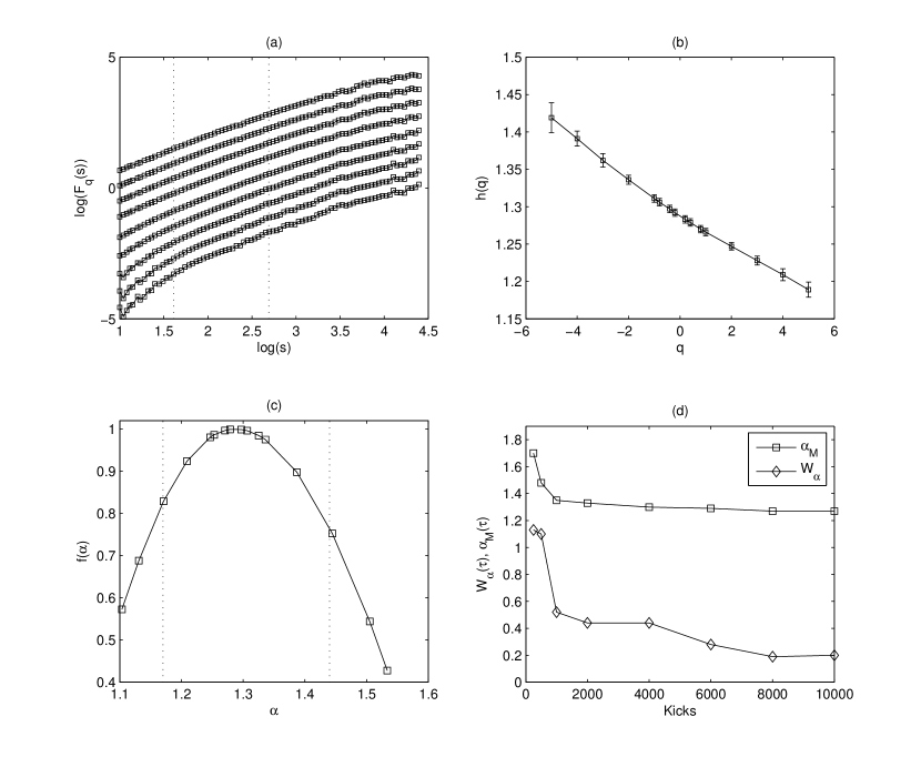
Figure 3: (a) The decimal logarithm of $F_{q}(s)$ with $q\in[-5,5]$ for the $\tau$ scanned series with $t=6000$. The fitting procedure was performed in the zone $\log(s)\in[1.6,2.7]$ (corresponding to $s\in[40,500]$). (b) The spectrum of the generalized Hurst exponents $h(q)$. (c) The $f(\alpha)$ spectrum with $\alpha_{M}=1.29$ and $W_{\alpha}=0.28$. (d) The variation of the multifractal parameters $\alpha_{M}$ and $W_{\alpha}$ with the interaction time. $\alpha_{M}$ shows a saturation towards the value $\alpha_{M}\approx 1.3$, while $W_{\alpha}$ tends to saturate around the value $W_{\alpha}\approx 0.2$.

A full analysis for $t=6000$ (see Figure 1) is shown in Figures 2 and 3 for the $\beta$ and $\tau$ scanned series, respectively. Tables 1 and 2 collect the multifractal parameters $\alpha_{M}$ and $W_{\alpha}$, which were computed for $t=250\ldots 10000$. Analogously to EPL68-04 , we defined $W_{\alpha}$ as the width of the parabolic form of $f(\alpha)$ between the points corresponding to $q=-3$ and $q=3$.

Figure 2(a) shows the scaling behaviour of the fluctuation function $F_{q}(s)$, with $q\in[-5,5]$. Here $s$ represents the index of the scanning parameter $\beta$, while the fit was performed in the zone $\log(s)\in[1.6,2.7]$ (corresponding to $s\in[40,500]$). In Figure 2(b) we report the dependence of $h(q)$ on $q$, revealing the multifractal nature of the data set. In order to better characterize the multifractality and to highlight how it changes among the different analyzed series, we have computed the MF spectrum $f(\alpha)$ (c.f. 2(c)). Figure 2(d) shows the variation of the multifractal parameters for the different interaction times considered. After a fast decrease, both the parameters tend to converge around the values $\alpha_{M}=1.29$ and $W_{\alpha}=0.2$ (see also Tab. 1). Very similar results were obtained for the $\tau$ scanned series (cf., Figure 3 and Table 2). Comparing the values of Tables 1 and 2 we can say that both the $\tau$ and the $\beta$ scanned series have essentially the same multifractality.

Even if we cannot a priori predict the asymptotic similarity between the two series of $\tau$ and $\beta$, we can a posteriori interpret this result: both parameters enter not equally yet similarly in the phase of the second factor on the right of eq. (2). As a consequence, the restriction of $\beta$ to the unit interval does make no difference to the, in principle, unboundedness of $\tau$ (in fact, to avoid different dynamical properties of the system, $\tau$ was chosen in a restricted window too, c.f. TMW2006 ).

In general, two types of multifractality can be distinguished, and both of them require different scaling exponents for small and large fluctuations. (I) The multifractality can be due to the broad probability density function for the values, and (II) it can also be due to different long range correlations for small and large fluctuations. The simplest way to distinguish between the mentioned two cases is to perform the analysis on a randomly reshuffled series. The shuffling destroys all the correlations, and the series with multifractals of type (II) will exhibit a monofractal behaviour with $h_{\mbox{{\tiny shuf}}}(q)=0.5$ and $W_{\alpha}=0$. On the contrary, multifractality of type (I) is not affected by the shuffling procedure. If both (I) and (II) are present the series will show a weaker multifractality than the original one.

We applied the shuffling procedure to the series showed in Figure 1. The procedure destroyed the multifractality of both series since for both the sequences we obtained $h(q)=0.51\pm 0.01$ for $q\in[-5,5]$. The dependence on $q$ was so weak that we were not able to compute any reliable $f(\alpha)$ spectrum, which, in this case, can be considered singular, i.e., with $W_{\alpha}\approx 0$.

V Conclusions

We studied the quantum kicked rotor, a paradigmatic model of quantum chaos, which describes the time evolution of cold atoms in periodically flashed optical lattices. Imposing absorbing boundary conditions allows one to probe the transport properties of the system, here expressed by the survival probability on a finite region in momentum space. For a fixed interaction time, the quantum survival probability depends sensitively on the parameters of the system, and our application of the detrended multifractal method shows that clear signatures of a multifractal scaling of the survival probability are found, as either the kicking period or quasimomentum is scanned. Our results generalize the previously predicted mono-fractal structure of the signal GT2001 ; TMW2006 ; BCGT2001 , by characterizing long-range correlations in the parametric fluctuations. In agreement with the monotonic increase of the box counting dimension with the interaction time $t$ and its saturation after $t\;{\scriptstyle{>\atop\sim}}\;5000$ observed in TMW2006 , we found a systematically decreasing value for the maximum $\alpha_{M}$ of the MF spectrum and of its widths $W_{M}$. Both of these two values also tend to saturate for $t\;{\scriptstyle{>\atop\sim}}\;5000$.

Future work along the lines of TMW2006 will be devoted to check in detail whether traces of the here predicted multifractality could be observed under real-life experimental conditions (e.g., for short interaction times and finite resolutions in the scanning parameter TMW2006 ).

VI Acknowledgments

S.W. acknowledges support by the Alexander von Humboldt Foundation (Feodor-Lynen Program) and is grateful to Carlos Viviescas and Andreas Buchleitner for their hospitality at the Max Planck Institute for the Physics of Complex Systems (Dresden) where part of this work has been done. A.F. is grateful to Holger Kantz and Nikolay Vitanov for their support and important suggestions. Furthermore we thank Riccardo Mannella for his helpful advice on the numerical procedure.

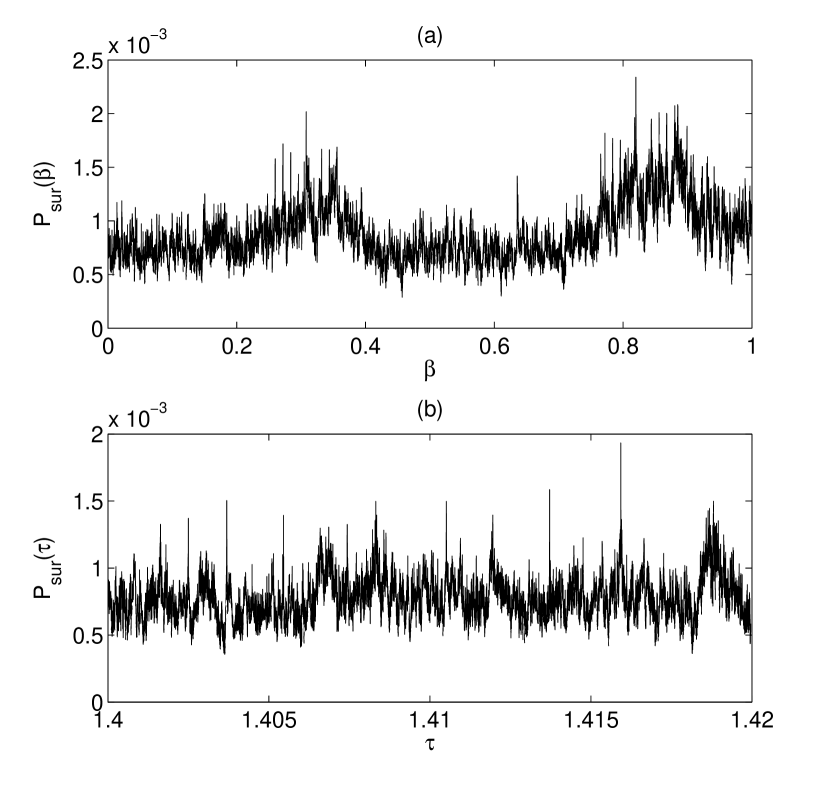
Figure 1: The series $P_{sur}(\beta)$ (a) and $P_{sur}(\tau)$ (b) after an interaction time of $t=6000$ kicks. Other paramters are $k=5$, and $\tau=1.4$ in (a) and $\beta=0$ in (b), respectively. Both sequences extend over $10^{5}$ sampling points along the shown intervals.

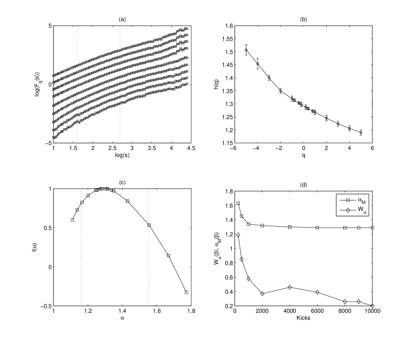
Figure 2: (a) The decimal logarithm of the fluctuation function $F_{q}(s)$ for $q\in[-5,5]$ for the $\beta$ scanned series after an interaction time of 6000 kicks. The fitting procedure was performed in the zone $\log(s)\in[1.6,2.7]$ (corresponding to $s\in[40,500]$). The curves were vertically shifted for better reading. (b) The spectrum of the generalized Hurst exponents $h(q)$; its strong dependence on $q$ indicates the multifractal behaviour. The error bars show the uncertainty arising from the fits to the curves in (a). (c) The $f(\alpha)$ spectrum with $\alpha_{M}=1.29$ and $W_{\alpha}=0.39$. The dotted lines indicate the $\alpha$ interval used to compute $W_{\alpha}$. (d) The multifractal parameters $\alpha_{M}$ and $W_{\alpha}$ as a function of the interaction time. After a strong, initial variation, the value $\alpha_{M}$ shows a saturation towards the value $\alpha_{M}\approx 1.3$. The width $W_{\alpha}$ shows approximately the same behaviour, and tends to saturate towards the value $W_{\alpha}\approx 0.2$.

Table 1: Multifractal parameters of the $\beta$-scanned data sets for different interaction times. The estimated error due to the fitting procedure described in section III is about $\pm 0.02$ for $\alpha_{M}$ and $\pm 0.05$ for $W_{\alpha}$.

	$\alpha_{M}$	$W_{\alpha}$
t=250	1.63	1.19
t=500	1.45	0.85
t=1000	1.34	0.58
t=2000	1.32	0.37
t=4000	1.30	0.46
t=6000	1.29	0.39
t=8000	1.29	0.26
t=10000	1.29	0.20

Table 2: Multifractal parameters of the $\tau$-scanned data sets for different interaction times (error estimates as stated for the preceding table).

	$\alpha_{M}$	$W_{\alpha}$
t=250	1.70	1.13
t=500	1.48	1.12
t=1000	1.35	0.9
t=2000	1.33	0.52
t=4000	1.30	0.44
t=6000	1.29	0.28
t=8000	1.27	0.19
t=10000	1.27	0.20

References

- (1) E. Ott, Chaos in Dynamical Systems, Cambridge University Press, Cambridge, 1993.
- (2) H. Kantz, T. Schreiber, Nonlinear Time Series Analysis, Cambridge University Press, Cambridge, 1997.
- (3) L. Pietronero, A. P. Siebesma, E. Tosatti, M. Zannetti, Phys. Rev. B 36, 5635 (1987); M. Schreiber, H. Grussbach, Phys. Rev. Lett. 67, 607 (1991), and refs. therein.
- (4) L. Schweitzer, P. Markoŝ, Phys. Rev. Lett. 95 (2005) 256805; J. A. Méndez-Bermidez, T. Kottos, Phys. Rev. B 72 (2005) 064108, and refs. therein.
- (5) R. Berkovitz, J. W. Kantelhardt, Y. Avishai, S. Havlin, A. Bunde, Phys. Rev. B 63 (2001) 085102.
- (6) M. Janssen, M. Metzler, M. R. Zirnbauer, Phys. Rev. B 59 (1999) 15636.
- (7) I. Guarneri, M. Terraneo, Phys. Rev. E 65 (2001) 015203(R).
- (8) A. Tomadin, R. Mannella, S. Wimberger, J. Phys. A 39 (2006) 2477.
- (9) M. Terraneo, Ph. D. Thesis, Università degli Studi di Milano 2001; I. Guarneri, M. Terraneo, S. Wimberger, unpublished.
- (10) F. Borgonovi, I. Guarneri, D. L. Shepelyansky, Phys. Rev. A 43, 4517 (1991); S. Wimberger, A. Krug, A. Buchleitner, Phys. Rev. Lett. 89 (2002) 263601; A. Ossipov, T. Kottos, T. Geisel, Europhys. Lett. 62, 719 (2003); S. E. Skipetrov, B. A. van Tiggelen, Phys. Rev. Lett. 96, 043902 (2006).
- (11) G. Benenti, G. Casati, I. Guarneri, M. Terraneo, Phys. Rev. Lett. 87 (2001) 014101.
- (12) B. V. Chirikov, Phys. Rep. 52 (1979) 263.
- (13) F. M. Izrailev, Phys. Rep. 196 (1990) 299.
- (14) F. L. Moore, J. C. Robinson, C. F. Bharucha, B. Sundaram, M. G. Raizen, Phys. Rev. Lett. 75 (1995) 4598; H. Ammann, R. Gray, I. Shvarchuck, N. Christensen, ibid. 80 (1998) 4111; J. Ringot, P. Szriftgiser, J. C. Garreau, D. Delande D, ibid. 85 (2000) 2741; M. Sadgrove, S. Wimberger, S. Parkins, R. Leonhardt, ibid. 94 (2005) 174103; M. B. d’Arcy et al, Phys. Rev. E 69 (2004) 027201.
- (15) S. Wimberger, I. Guarneri, S. Fishman, Nonlinearity 16 (2003) 1381.
- (16) G. J. Duffy, S. Parkins, T. Muller, M. Sadgrove, R. Leonhardt, A. C. Wilson, Phys. Rev. E 70 (2004) 056206; better control of the quasimomentum was recently realized by a method decribed in C. Ryu et al., Phys. Rev. Lett. 96 (2006) 160403.
- (17) C. K. Peng, S. V. Buldriev, S. Havlin, M. Simons, H. E. Stanley, A. L. Goldberger, Phys. Rev. E 49 (1999) 1685.
- (18) J. W. Kantelhardt, S. A. Zsciegner, E. Koscienly-Bunde, S. Havlin, A. Bunde, H. E. Stanley, Physica A 316 (2002) 87.
- (19) R. K. Kavasseri, R. Nagarajan, Chaos Solitons and Fractals 24 (2005) 165-173.
- (20) D. Makowieca, R. Galaska, A. Dudkowskaa, A. Rynkiewiczb, M. Zwierza, Physica A (2006) in press (Doi:10.1016/j.physa.2006.02.038).
- (21) J. W. Lee, K. E. Lee, P. A. Rikvold, Physica A 364 (2006) 355-361.
- (22) J. L. McCauley, Chaos, Dynamics, and Fractals : An Algorithmic Approach to Deterministic Chaos, Cambridge University Press, Cambridge, 1994.
- (23) N. K. Vitanov, K. Sakai, E. D. Yankulova, J. of Theor. and Appl. Mechanics, 35 (2005) 2.
- (24) J. Feder, Fractals, Plenum Press, New York, 1988.
- (25) R. B. Govindan, H. Kantz, Europhys. Lett. 68 (2004) 184.