Elastic response of a nematic liquid crystal to an immersed nanowire

Abstract

We study the immersion of a ferromagnetic nanowire within a nematic liquid crystal using a lattice Boltzmann algorithm to solve the full three-dimensional equations of hydrodynamics. We present an algorithm for including a moving boundary, to simulate a nanowire, in a lattice Boltzmann simulation. The nematic imposes a torque on a wire that increases linearly with the angle between the wire and the equilibrium direction of the director field. By rotation of these nanowires, one can determine the elastic constants of the nematic.

I Introduction

In a pioneering theoretical study in 1973 de Gennes and Brochard looked at the effect of dispersing long rod-like particles in a liquid crystal Brochard and de Gennes (1970). Despite interesting predictions on ferronematics and ferrocholesterics, little experimental work was done at the time. Very recently, however, there has been a resurgence of interest in this subject motivated by the advent of nanofabrication techniques to make such particles Hamatsu et al. (1996); Cui and Lieber (2001); Tanase et al. (2001); Hochbaum et al. (2005); Gorby et al. (2006). Early results are already very encouraging. For example, solutions of just $0.1-0.2$wt% of carbon nanotubes in E7 have shown a dramatic increase ($\sim 30^{o}$) in the nematic-isotropic transition temperature Lynch and Patrick (2002); Duran et al. (2005).

Recent research on the inclusion of spherical particles in a nematic have shown that unique interactions between particles which can lead to self-assembly Poulin et al. (1997a); Loudet and Poulin (2001); Kossyrev et al. (2006). There has also been considerable interest in generalizing micro-rheological tools, such as examining the fluctuations of microspheres to measure local viscosities Poulin et al. (1997b); Kachynski et al. (2003). However, there are complications in using spheres for micro-rheology in an anisotropic fluid like a liquid crystal that are not present in isotropic fluids. First, boundary conditions at the surface of the sphere typically induce defects either on or close to the surface of the sphere Poulin et al. (1997a); Poulin and Weitz (1998); Mondain-Monval et al. (1999); Gu and Abbott (2000). These significantly modify the director field of the liquid crystal thus making the sphere far from a passive probe. Second, these spheres are typically manipulated via laser traps Muševič et al. (2004); Yada et al. (2004); Smalyukh et al. (2005). However, the electric fields required to trap a sphere also strongly affect the alignment of the liquid crystal Škarabot et al. (2006) again making the system non-passive.

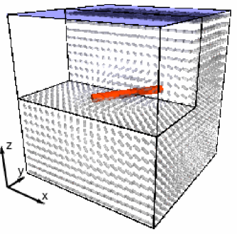
Figure 1: Schematic of a sample cell in our simulation. The dimensions are $1.25\mu m\times 1.25\mu m\times 1.25\mu m$. Two rigid surfaces are located at $z=0$ and $z=L$ and there is periodic boundaries in the $xy-$plane. In the middle of the cell is a ferromagnetic nanowire $625nm$ in length and approximately $88nm$ in diameter. The top front quarter has been removed for clarity.

Recent experiments on nickel nanowires in a liquid crystal have shown that they can be manipulated with magnetic fields and that the torque exerted on the wire by the liquid crystal can be directly measured Lapointe et al. (2004, 2005). The magnetic fields required to manipulate these ferromagnetic wires are typically very small, $\sim 5$ Gauss Lapointe et al. (2004), much less than that required to align the liquid crystal ($\sim 3500$ Gauss for the Frederik’s transition in 5CB in a cell with thickness 10$\mu m$de Gennes and Prost (1993)). Further, when the wire is aligned with the director field, it causes no distortion. Thus, the use of such an anisotropic particle is ideal for doing micro-rheology in an anisotropic fluid. By manipulating the wires immersed in the nematic it should be possible to infer the local viscous and elastic properties of the liquid crystal.

Simulations of colloids in liquid crystals have also recently been performed, but most have focused on homeotropic anchoring to the colloid. Monte Carlo simulations were performed on rods of infinite length Andrienko et al. (2002). Also, there is work on soft two-dimensional cylinders using lattice Boltzmann Lishchuk et al. (2004) and FEM simulations on hard cylinders Hung et al. (2006). All these works used homeotropic anchoring which leads to saturn ring-like defects along and around the cylinder. In this paper we focus on the cylinder, or wire, with boundary conditions where the nematic aligns with the long axis of the wire. The lack of defect formation from this configuration makes it ideal for microrheological applications as it can now measure the linear response of an unperturbed background.

Analytic calculations of the response of a liquid crystal to an immersed particle can only be carried out by imposing rather unrealistic assumptions. This makes the use of simulations necessary to understand precisely what is measured in experiments. Lattice Boltzmann schemes have proved to be very successful in simulations of complex fluids Chen and Doolen (1998), including liquid crystals Denniston et al. (2000, 2001). We will examine a system similar to the experimental setup described in Lapointe et al. (2004), as shown in Figure 1. We have a simulation cell with rigid surfaces for boundaries at $z=0$ and $z=L$, where $L$ is the height of the cell. The surfaces impose a preferred aligned direction for the nematic liquid crystal. The $xy-$plane has periodic boundaries in both directions. At the center of the cell, a small ferromagnetic nickel wire will be immersed. With the system in equilibrium, we can rotate the magnetic field in the $z$ plane to rotate the wire within the box. Using the response function of the imposed torque, we are able to measure the elastic properties of the nematic liquid crystal.

II Equations of Motion

Liquid crystals can be characterized by the second moment of the orientation of the constituent molecules $\hat{p}$, in terms of a local tensor order parameter ${\bf Q}$ where $Q_{\alpha\beta}=\langle\hat{p}_{\alpha}\hat{p}_{\beta}-\frac{1}{3}\delta_{\alpha\beta}\rangle$. We use angular brackets to denote a coarse-grained thermal average. Greek indices will be used to represent Cartesian components of vectors and tensors and the usual summation over repeated indices is assumed. ${\bf Q}$ is a traceless symmetric tensor. We label its largest eigenvalue $\frac{2}{3}q$ so that $0<q<1$. $q$ describes the magnitude of order along Q’s principle eigenvector $\hat{\bf n}$, referred to as the director.

The nematic order parameter evolves according to the convective-diffusive equation Beris and Edwards (1994)

$$(\partial_{t}+{\vec{u}}\cdot{\bf\nabla}){\bf Q}-{\bf S}({\bf W},{\bf Q})=D_{r}{\bf H}$$ (1)

where $D_{r}$ is a collective rotational diffusion constant. The order parameter distribution can be both rotated and stretched by flow gradients described by

$${\bf S}({\bf W},{\bf Q}) = (\chi{\bf A}+{\bf\Omega})({\bf Q}+{\bf I}/3)+({\bf Q}+{\bf I}/3)(\chi{\bf A}-{\bf\Omega})$$ (2)

$$-2\chi({\bf Q}+{\bf I}/3){\mbox{Tr}}({\bf A}({\bf Q}+{\bf I}/3))$$

where ${\bf A}=({\bf W}+{\bf W}^{T})/2$ and ${\bf\Omega}=({\bf W}-{\bf W}^{T})/2$ are the symmetric part and the anti-symmetric part respectively of the velocity gradient tensor $W_{\alpha\beta}=\partial_{\beta}u_{\alpha}$. $\chi$ is a constant which depends on the molecular details of a given liquid crystalfootnote1 .

The term on the right hand side of Eqn. (1) describes the relaxation of the order parameter towards the minimum of the free energy. The molecular field ${\bf H}$ that provides the driving motion is related to the variational derivative of the free energy by

$${\bf H}=-\frac{\delta\mathcal{F}}{\delta{\bf Q}}+\frac{{\bf I}}{3}\textrm{Tr}\frac{\delta\mathcal{F}}{\delta{\bf Q}}.$$ (3)

The symmetry and zero trace of ${\bf Q}$ and ${\bf H}$ are exploited for simplification.

The equilibrium properties of a liquid crystal can be described in terms of the Landau-de Gennes free energy de Gennes and Prost (1993)

$$\mathcal{F}=\int_{V}dV\left\{F_{B}+F_{E}\right\}+\int_{\partial V}dSF_{S}.$$ (4)

$F_{B}$ describes the bulk free energy

$$F_{B} = \frac{A_{0}}{2}(1-\frac{\gamma}{3})Q_{\alpha\beta}^{2}-\frac{A_{0}\gamma}{3}Q_{\alpha\beta}Q_{\beta\gamma}Q_{\gamma\alpha}$$ (5)

$$+\frac{A_{0}\gamma}{4}(Q_{\alpha\beta}^{2})^{2}.$$

The bulk free energy describes a liquid crystal with a first order phase transition at $\gamma=2.7$ from the isotropic to nematic phase Doi and Edwards (1988). When $\gamma>3$ the isotropic phase is completely unstable. Unless noted, we use $\gamma=3.2$ and $A_{0}=1.5\times 10^{5}pN/(\mu m)^{2}$ which leads to $q=0.555$ in the unstressed equilibrium uniaxial case. We also used higher values of $q$ and found no qualitative difference.

The free energy also contains an elastic term,

$$F_{E}=\frac{L_{1}}{2}(\partial_{\alpha}Q_{\beta\gamma})^{2}+\frac{L_{2}}{2}(\partial_{\alpha}Q_{\alpha\gamma})(\partial_{\beta}Q_{\beta\gamma})+$$

$$\frac{L_{3}}{2}Q_{\alpha\beta}(\partial_{\alpha}Q_{\gamma\epsilon})(\partial_{\beta}Q_{\gamma\epsilon}),$$ (6)

where the $L$’s are the material specific elastic constants. It is straightforward to map $L$’s to the Frank elastic constants (the splay elastic constant $K_{1}$, the twist elastic constant $K_{2}$, and the bend elastic constant $K_{3}$)Beris and Edwards (1994). The one elastic constant approximation $K_{1}=K_{2}=K_{3}=K$ can be easily achieved by setting $L_{1}>0$, $L_{2}=L_{3}=0$ footnote2 . One advantage of simulations is the ease of switching between such an approximation commonly used in analytical work and the full equations necessary to compare to experiment.

At the surfaces of the system we assume a pinning potential

$$F_{S}=\frac{1}{2}\alpha_{s}(Q_{\alpha\beta}-Q_{\alpha\beta}^{o})^{2},$$ (7)

where ${\bf Q}^{o}$ has the form

$$Q_{\alpha\beta}^{o}=q^{o}\left(n^{o}_{\alpha}n^{o}_{\beta}-\frac{\delta_{\alpha\beta}}{3}\right),$$ (8)

and $q^{o}$ is set to the equilibrium bulk value $q$. This corresponds to a preferred direction ${\bf n}^{o}$ for the director at the surface. Typically we set $\alpha_{s}=6.33\times 10^{4}pN/\mu m$, which corresponds to the strong pinning limit where $Q\approx Q_{o}$ at the boundaries.

Inclusion of the wire in the system will be approximated as a moving boundary. We will use a pining potential similar to (7) for pining the director field of the liquid crystal to the long axis of the wire. This will be discussed in greater detail below and in Section III.2.

The fluid momentum obeys the continuity

$$\partial_{t}\rho+\partial_{\alpha}\rho u_{\alpha}=0$$ (9)

and the Navier-Stokes equation

$$\rho(\partial_{t}+u_{\beta}\partial_{\beta})u_{\alpha}=\partial_{\beta}\tau_{\alpha\beta}+\partial_{\beta}\sigma_{\alpha\beta}$$

$$\quad+\eta\partial_{\beta}((1-3\partial_{\rho}P_{0})\partial_{\gamma}u_{\gamma}\delta_{\alpha\beta}+\partial_{\alpha}u_{\beta}+\partial_{\beta}u_{\alpha})$$ (10)

where $\rho$ is the fluid density and $\eta=\rho\tau_{f}/3$ is an isotropic viscosity. The form of this equation is not dissimilar to that for a simple fluid (anisotropic viscosities arise due to terms in $\sigma_{\alpha\beta}$. However the details of the stress tensor reflect the additional complications of liquid crystal hydrodynamics. There is a symmetric contribution

$$\sigma_{\alpha\beta} = -P_{0}\delta_{\alpha\beta}$$ (11)

$$- \xi H_{\alpha\gamma}(Q_{\gamma\beta}+{1\over 3}\delta_{\gamma\beta})-\xi(Q_{\alpha\gamma}+{1\over 3}\delta_{\alpha\gamma})H_{\gamma\beta}$$

$$+ 2\xi(Q_{\alpha\beta}+{1\over 3}\delta_{\alpha\beta})Q_{\gamma\epsilon}H_{\gamma\epsilon}-\partial_{\beta}Q_{\gamma\nu}{\delta{\cal F}\over\delta\partial_{\alpha}Q_{\gamma\nu}}$$

and an antisymmetric contribution

$$\tau_{\alpha\beta}=Q_{\alpha\gamma}H_{\gamma\beta}-H_{\alpha\gamma}Q_{\gamma\beta}.$$ (12)

These additional terms can be mapped onto the Erickson-Leslie equations to give the Leslie coefficients Denniston et al. (2001). The isostatic pressure $P_{o}$ is constant in the simulations to a very good approximation, consistent with the liquid crystal being incompressible.

At the surface of the wire we assume a molecular surface field of a form similar to Eqn (7) where

$$H^{w}=w_{s}({\bf Q}-{\bf Q}^{w}),$$ (13)

and $Q^{w}_{\alpha\beta}=q^{w}(m_{\alpha}m_{\beta}-\delta_{\alpha\beta}/3)$. The director ${\bf m}$ of ${\bf Q}^{w}$ is fixed along the long axis of the wire and $q^{w}$ is set to the equilibrium bulk value

$$q=\frac{1}{4}\left(1-3\sqrt{1-\frac{8}{3\gamma}}\right).$$ (14)

For the uniaxial case, where $Q_{\alpha\beta}=q\left(n_{\alpha}n_{\beta}-\frac{\delta_{\alpha\beta}}{3}\right)$, the torque on the liquid crystal due to the presence of the wire is easily shown to be de Gennes and Prost (1993)

$${\bm{\Gamma}}={\bf m}\times{\bf h}^{w},$$ (15)

where ${\bf m}$ is the unit direction vector of the wire, and

$$h_{\mu}^{w}=q^{w}\left(m_{\beta}H_{\mu\beta}^{w}+m_{\alpha}H_{\alpha\mu}^{w}\right).$$ (16)

In our simulations, the torque is determined in system variables by

$$\Gamma_{\alpha} = 2[Q_{\alpha\beta}H_{\alpha\gamma}^{w}-Q_{\alpha\gamma}H_{\alpha\beta}^{w}+H_{\beta\gamma}^{w}(Q_{\beta\beta}-Q_{\gamma\gamma})+$$ (17)

$$\quad Q_{\beta\gamma}(H_{\beta\beta}^{w}-H_{\gamma\gamma}^{w})],$$

which can be easily shown to be equivalent to Eqn. (15) in the uniaxial case.

The motion of the wire is performing a balancing act between forces. Its motion is described by

$$\Lambda(\hat{{\bf m}}\times\dot{\hat{{\bf m}}})=-({\bm{\Gamma}}-({\bm{\Gamma}}\cdot\hat{{\bf m}})\hat{{\bf m}})+{\bm{\mu}}\times{\bf B}$$ (18)

where $\Lambda$ is a rotational viscosity and ${\bm{\mu}}\times{\bf B}$ is the torque on the wire due it its magnetic moment ${\bm{\mu}}$ in the applied magnetic field. The $(\Gamma\cdot{\bf m}){\bf m}$ term is zero but it’s presence enhances the numerical stability of the scheme. In principle, $\Lambda$ should depend on the orientation of the wire Lapointe et al. (2005), but in this study we are interested in the steady state solution. As such, this term only serves to move the wire between steady states here.

III Numerical Implementation

III.1 The Lattice Boltzmann Algorithm for Liquid Crystal Hydrodynamics

We summarize a lattice Boltzmann scheme which reproduces Eqns. (1), (9), and (10) to second order. The reader only interested in the results can safely skip over this section. We defined two distribution functions $f_{i}({\bf x})$ and ${\bf G}_{i}({\bf x})$ where $i$ labels the lattice directions from site ${\bf x}$. In two dimensions, we choose a nine-velocity model on a square lattice with velocity vectors $\overrightarrow{e}_{i}=(\pm 1,0),(0,\pm 1),(\pm 1,\pm 1),(0,0)$. For three-dimensional systems, a 15-velocity model on a cubic lattice with lattice vectors $\overrightarrow{e}_{i}=(0,0,0),(\pm 1,0,0),(0,\pm 1,0),(0,0,\pm 1),(\pm 1,\pm 1,\pm 1)$ is chosen. Physical variable are defined as moments of the distribution functions by

$$\rho=\sum_{i}f_{i},\qquad\rho u_{\alpha}=\sum_{i}f_{i}e_{i\alpha},\qquad{\bf Q}=\sum_{i}{\bf G}_{i}.$$ (19)

The distribution functions evolve in a time step $\Delta t$ according to

$$f_{i}({\vec{x}}+{\vec{e}}_{i}\Delta t,t+\Delta t)-f_{i}({\vec{x}},t)=$$

$$\quad\frac{\Delta t}{2}\left[{\cal C}_{fi}({\vec{x}},t,\left\{f_{i}\right\})+{\cal C}_{fi}({\vec{x}}+{\vec{e}}_{i}\Delta t,t+\Delta t,\left\{f_{i}^{*}\right\})\right],$$

(20)

$${\bf G}_{i}({\vec{x}}+{\vec{e}}_{i}\Delta t,t+\Delta t)-{\bf G}_{i}({\vec{x}},t)=$$

$$\quad\frac{\Delta t}{2}\left[{\cal C}_{{\bf G}i}({\vec{x}},t,\left\{{\bf G}_{i}\right\})+{\cal C}_{{\bf G}i}({\vec{x}}+{\vec{e}}_{i}\Delta t,t+\Delta t,\left\{{\bf G}_{i}^{*}\right\})\right].$$

(21)

This represents free streaming with velocity ${\vec{e}}_{i}$ and a collision step which allows the distribution to relax towards equilibrium. $f_{i}^{*}$ and ${\bf G}_{i}^{*}$ are first order approximations to $f_{i}({\vec{x}}+{\vec{e}}_{i}\Delta t,t+\Delta t)$ and ${\bf G}_{i}({\vec{x}}+{\vec{e}}_{i}\Delta t,t+\Delta t)$ respectively. They are obtained by using only the collision operator ${\cal C}_{fi}({\vec{x}},t,\left\{f_{i}\right\})$ on the right of Equation (20) and a similar substitution in (21). Discretizing in this way, which is similar to a predictor-corrector scheme, has the advantages that lattice viscosity terms are eliminated to second order and that the stability of the scheme is significantly improved.

The collision operators are taken to have the form of a single relaxation time Boltzmann equationChen and Doolen (1998), together with a forcing term

$${\cal C}_{fi}({\vec{x}},t,\left\{f_{i}\right\}) = -\frac{1}{\tau_{f}}(f_{i}({\vec{x}},t)-f_{i}^{eq}({\vec{x}},t,\left\{f_{i}\right\}))$$ (22)

$$\quad+p_{i}({\vec{x}},t,\left\{f_{i}\right\}),$$

$${\cal C}_{{\bf G}i}({\vec{x}},t,\left\{{\bf G}_{i}\right\}) = -\frac{1}{\tau_{g}}({\bf G}_{i}({\vec{x}},t)-{\bf G}_{i}^{eq}({\vec{x}},t,\left\{{\bf G}_{i}\right\}))$$ (23)

$$\quad+{\bf M}_{i}({\vec{x}},t,\left\{{\bf G}_{i}\right\}).$$

The form of the equations of motion and thermodynamic equilibrium follow from the choice of the moments of the equilibrium distributions $f^{eq}_{i}$ and ${\bf G}^{eq}_{i}$ and the driving terms $p_{i}$ and ${\bf M}_{i}$. Full details of the algorithm can be found in Denniston et al. (2001, 2004) for two-dimensional and three-dimensional simulations respectively.

III.2 Description of the Nanowire

When a particle is suspended in a nematic liquid, anchoring boundary conditions at the particle’s surface dictate the direction of the director field in the vicinity of the particle. Using a pinning potential of the form of Eqn (7), with $n_{o}$ along the long axis of the wire, ensures the director of the nearby nematic is aligned to the nanowire. The nanowire is ferromagnetic, enabling an external magnetic field to rotate the wire within the system.

A numerical algorithm for simulating the inclusion of a nanowire in a liquid crystal system is presented in this section. We could use an adaptive mesh with boundaries aligned on the wire but since the wire diameter is quite small ($\sim 100\,nm$), we decide against this method due to the small resolutions required. For instance, if there were 10 mesh points spanning the diameter of wire we would be approaching molecular resolution. The alternative is to pixelate a line onto a grid, a problem common in computer graphics. First we will start off with a two-dimensional description, then expand to three dimensions. We will describe both a standard Bresenham line algorithm Bresenham (1965), expanded upon by Wu Wu (1991), to produce lines on a two-dimensional surface and then we will present our current algorithm.

III.2.1 Computer Graphics Method

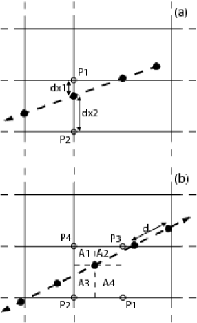
Figure 2: (a) Example of the Brensenham anti-aliased line drawing algorithm. If the slope is less one, the nodes are positioned along vertical lattice intersections, shown as the open dots at positions $P1$ and $P2$. Value of the lattice nodes are inversely proportional to the distance from the lattice nodes to the wire nodes. (e.g. $P1=dx_{2}/dx$) For a slope greater than one, the horizontal lattice intersections are used. (b) Sample cell of a two-dimensional system with an intersecting wire. Along the wire, nodes are positioned at fixed distances $d$ apart to interact with the lattice nodes. Each node is affected by the wire proportionally by the opposite enclosed area relative to the cell area. (e.g. $P2$ is affected from the wire by an amount $A2/dx^{2}$.)

The standard algorithm for pixelating a line is based on Bresenham’s algorithm, generalized by Wu Bresenham (1965). This is illustrated in Fig 2(a). When the slope of the line is less than 1, the points where the wire crosses vertical grid lines are marked. The value of a particular wire node is proportional to the distance of the lattice crossing to the opposite node over the cell height. For example, the value at $P2=dx_{1}/dx$ in Figure 2(a). The endpoints of the wire prove to be more cumbersome, involving extrapolation to the next grid line and weighting the points. If the slope exceeds one, we swap the roles of $x$ and $y$ and exchange the vertical lattice crossings, with horizontal lattice crossings. This method is easy to implement in two-dimensions. Unfortunately it is not easily generalized for three dimensional systems. Other problems arise due to the fact that the number of nodes along the wire is not conserved as the wire rotates. These issues will described in more detail in the next section.

III.2.2 Node distribution method

Placing a wire within the simulation will require pixelation to map it onto the lattice coordinates. Our method is illustrated in Fig 2(b). We divide the wire into a fixed number of nodes $N$. The solid dots are the location of the nodes along the wire separated by a distance $d$, where $d$ is incommensurate with the lattice spacings. Typically we have used $d=0.2\phi_{0}\,dx$, where $\phi_{0}=0.618\cdots$ is the golden mean. The wire nodes are then distributed to the corners of the cell in which they reside. To distribute the wire points to the closest lattice coordinates, the ratio of the opposite area from the node over the cell area will be calculated (Ex. $P1=A1/dx^{2}$). It is easy to see that the node weight thus defined varies smoothly from 0, when the wire node is at the opposite corner of the cell, to 1, when the wire node goes through the lattice point in question. This is done for all nodes along the nanowire. If multiple nodes affect a single lattice coordinate, the summation of their distributed values is used. Although the description above is for a two dimensional system, it is easily generalized to three dimensions where ratios of opposite volumes to the cell volume is used instead, and is the method employed in our simulations.

In three dimensions an area of fluid will be displaced and affected by the wire. To give the wire a lateral dimension greater than $dx$, we simulated many smaller wire strands in unison for the same effect. A diagram of three smaller strands forming a single wire is shown in Figure 3. In our simulations we use five strands in unison to form the nanowire. The white bands represent where the nodes lie. Each strand, from end to end, is coiled about the central axis by $2\pi$. This twist on the strands helps make the wire nodes even more incommensurate with the underlying lattice, something that turns out to be highly desirable for producing a smooth response.

Figure 3: Three chiral wires are shown together to simulate one larger wire. The white spaces are sample locations of the nodes along the smaller wires. To avoid commensurability with the lattice, the node distance is irrational. Chirality of the wire is also included to avoid commensurability issues. Each small wire is coiled by $2\pi$ about the central axis from end to end.

We want the surface energy of the wire to be independent of the way it is discretized. In other words, independent of the number of strands and nodes used (assuming a sufficiently high number) and independent of the orientation with respect to the lattice (i.e. if we rotate the numerical mesh but keep all the fields fixed). This requires that the integral of $H^{w}$, from Eqn. (13), over the surface of the wire be independent of the orientation of the wire with respect to the underlying lattice. This will be the case if the discretization of $\oint a_{s}d\textrm{A}$ is a constant independent of orientation and wire discretization, where $a_{s}$ is proportional to the surface area per node. To calculate $a_{s}$, we have

$$\oint a_{s}d\textrm{A}=2\pi rL=\sum_{i_{w},i_{n}}a_{s}$$ (24)

where $r$ and $L$ are the radius and length of the wire respectively, $i_{w}$ is the index for the wire strand, and $i_{n}$ is the index for the nodes on wire $i_{w}$. As a result, $\sum_{i_{w},i_{n}}$ the total number of nodes in all the strands. Solving for $a_{s}$ gives

$$a_{s}=\frac{2\pi rd}{N_{s}},$$ (25)

where $d$ is the node spacing along the strands and $N_{s}$ is the number of strands used to create the wire.

IV Results

IV.1 Theory

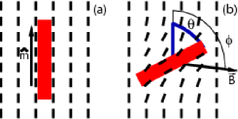
Figure 4: (a) A schematic of the wire immersed in the nematic (black dashed) at equilibrium. The magnetic field, the wire, and the director field of the nematic are all aligned along the same direction. (b) Introducing a magnetic field at angle $\phi$, the wire reorients to an angle $\theta$ balancing the magnetic and elastic torques on the wire. This leads to distortions in the nematic around the wire.

With no applied field, the long axis of the wire should line up parallel with the director, as shown in Figure 4 (a). Distortions in the orientation of the wire from this position, as in Figure 4 (b) will cost elastic energy. The director distorts to satisfy the boundary condition at the wire surface by introducing an elastic torque $\Gamma$ on the system.

In the equilibrium case where ${\bf Q}$ is uniaxial, $Q_{\alpha\beta}=\frac{3}{2}q(n_{\alpha}n_{\beta}-\frac{1}{3}\delta_{\alpha\beta})$, the elastic free energy density (6) can be rewritten as

$$F_{el} = \frac{1}{2}\left[K_{1}({\bm{\nabla}}\cdot{\bf n})^{2}+K_{2}({\bf n}\cdot{\bm{\nabla}}\times{\bf n})^{2}\right.$$ (26)

$$\left.+K_{3}({\bf n}\times{\bm{\nabla}}\times{\bf n})^{2}\right].$$

For analytic work it is useful to work in the approximation where the elastic constants are all equal. In that case, choosing the director field ${\bf n}$ to have the form $n_{x}=\cos\theta\sin\psi$, $n_{y}=\sin\theta\sin\psi$, and $n_{z}=\cos\psi$ then (26) can take the form

$$F_{el} = \frac{1}{2}K\left[({\bm{\nabla}}\psi)^{2}+\sin^{2}\psi({\bm{\nabla}}\theta)^{2}\right.$$ (27)

$$+\left.2\sin\psi\ {\bf n}\cdot({\bm{\nabla}}\theta\times{\bm{\nabla}}\psi)\right].$$

Minimizing (27) with respect to the angles leads to two equations of equilibrium Chandrasekhar (1992),

$$\nabla^{2}\psi-\sin\psi\cos\psi(\nabla\theta)^{2}=0$$ (28)

$$\sin\psi\nabla^{2}\theta+2\cos\psi\nabla\psi\cdot\nabla\theta=0.$$ (29)

In equilibrium, the nanowire will be positioned in the middle of the sample cell parallel to the top and bottom surfaces. Using the coordinate system shown in Figure 1, $\psi=\frac{\pi}{2}$ in equilibrium. If we assume that rotating the wire in the plane parallel to the walls produces no out-of-plane deformations, then $\psi$ will remain constant at $\pi/2$. Under this assumption Eqn. (28) and (29) reduce to simply the Laplacian

$$\nabla^{2}\theta=0.$$ (30)

If we further assume that the shape of the wire can be approximated as a prolate spheroid, the equations can be solved analytically. The appropriate coordinate change is then

$$r_{\pm}=\sqrt{\left(z\pm\frac{a}{2}\right)^{2}+x^{2}+y^{2}}$$ (31)

$$\xi=\frac{r_{+}+r_{-}}{a}$$ (32)

$$\eta=\frac{r_{+}-r_{-}}{a}$$ (33)

$$\Xi=\tan^{-1}\left(\frac{y}{x}\right),$$ (34)

where $a$ is the interfocal distance. Setting $\theta_{o}$ to a constant equal to the wire orientation over the surface (i.e. ${\bf m}=(\cos\theta_{o},\sin\theta_{o},0)$), the Laplacian (30) becomes easily solvable Morse and Feshbach (1953) with solution

$$\theta=\theta_{o}\frac{\ln\left(\frac{\xi+1}{\xi-1}\right)}{\ln\left(\frac{\xi_{o}+1}{\xi_{o}-1}\right)},$$ (35)

where the constant $\xi_{o}$ defines the prolate spheroidal surface. From equilibrium, we integrate the elastic free energy density (27) over all space,

$$U_{el} = \frac{K}{2}\int dV(\nabla\theta)^{2}$$ (36)

$$= 2\pi aK\theta_{o}^{2}\left[\ln\frac{\xi_{o}+1}{\xi_{o}-1}\right]^{-1},$$

which results in an expression for the potential of a prolate spheroidal inclusion in a nematic.

In the approximation that the three elastic constants are equal, $K_{1}=K_{2}=K_{3}=K$, Brochard and de Gennes Brochard and de Gennes (1970) calculated the energy involved in considering a long inclusion, such as a wire, within a nematic as a function of the inclusions orientation. In the case the anchoring at the surface was along the long axis of the wire, they exploited an analogy from electrostatics of an object at fixed potentials to predict that the energy varies with the angle of orientation as

$$U_{el}=2\pi CK\theta^{2},$$ (37)

where $C$ is the capacitance of the wire. Equating (36) and (37), and making use of Eqn. (31) and (32), the capacitance is

$$C = a\left[\ln\frac{\xi_{o}+1}{\xi_{o}-1}\right]^{-1}$$ (38)

$$= 2L\sqrt{1-\left(\frac{R}{L}\right)^{2}}\left[\ln\left(\frac{1+\sqrt{1-\left(\frac{R}{L}\right)^{2}}}{1-\sqrt{1-\left(\frac{R}{L}\right)^{2}}}\right)\right]^{-1},$$ (39)

where $R$ and $L$ are the radius and length of the wire respectively. In the limit $\frac{R}{L}\rightarrow 1$ the capacitance is simply $C\rightarrow R$, that of a sphere, as expected. As $\frac{R}{L}\rightarrow 0$, the capacitance is

$$C\approx\frac{L}{\ln\left(\frac{2L}{R}\right)},$$ (40)

which is not the result Brochard and deGennes had attained, their result containing two incorrect factors of 2.

Although Eqn. (40) is the capacitance for a prolate ellipsoid, the wire in our system has a shape of a right cylinder. It is not possible to solve Laplace’s equation exactly for this shape, but expanding in $1/\zeta=1/\ln(\frac{2L}{R})$, JacksonJackson (2000) derived an approximate expression,

$$C = L\left\{\frac{1}{\zeta}+\frac{1}{\zeta^{2}}(1-\ln 2)\right.$$ (41)

$$+\left.\frac{1}{\zeta^{3}}\left[1+(1-\ln 2)^{2}-\frac{\pi^{2}}{12}\right]+O(1/\zeta^{4})\right\}.$$

For high aspect ratio wires, both Eqn. (40) and (41) are equivalent. As we shall see below, for low aspect ratio wires there is significant differences between the two equations and Eqn. (41) should be used instead.

IV.2 Torque on a nanowire in the simulations

In our simulations we will first try to replicate as closely as possible the theoretical results of the previous subsection. To do this we will first work in the one elastic constant limit and then move on to more realistic situations. This will demonstrate the ability of the node distribution algorithm to reproduce both the analytic results and the results from experiments.

We start with a wire aligned with the nematic director field in equilibrium, as shown in Figure 4(a). A magnetic field aligned in the direction of the long axis of the wire is introduced and slowly rotated in the $xy-$plane (See the schematic in Fig. 4(b) and the 3D simulation in Fig. 1 for reference). Taking $L_{2}=L_{3}=0$, to work in the one-elastic constant approximation, and if there is no out-of-plane distortion, a measurement of the torque on the wire from the nematic as a function of rotation angle should yield the elastic constant, assuming the capacitance of the wire is known. Using Eqn (37) for the potential energy results in a torque on a wire not aligned with the nematic,

$$\Gamma=\frac{\partial U}{\partial\theta}=4\pi CK\theta.$$ (42)

Eliminating the dependence on $\theta$, one can simply measure the value of the elastic constant via,

$$\ \frac{\partial\Gamma}{\partial\theta}=4\pi KC.$$ (43)

Thus, if $K$ is known one can determine $C$ or vice versa.

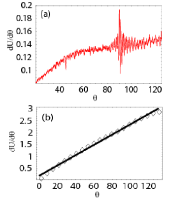
Figure 5: (a)Wu’s algorithm only works in 2-dimensions. The system is $1.25\mu m\times 1.25\mu m$ with a plate of length $0.675\mu m$. The torque clearly exhibits commensurabilty problems along certain orientations of the wire. (b) Using the algorithm described in Section III.2.2, one notices a smooth torque along a rotation. The are no indications of any commensurabilty problems as in Wu’s algorithm. The system is $1.25\mu m\times 1.25\mu m\times 1.25\mu m$ with a wire of length $0.675\mu m$. The one elastic constant approximation is used with $K=10.72pN$. To measure the slope a least squares fit is performed from the 0 to $\sim$2 radians.

Using the two methods described in Sections III.2.1 and III.2.2, we can simulate a wire in our system and measure the torque imposed by the nematic. The results are shown in Fig. 5. It should be immediately apparent that using the algorithm borrowed from the graphics industry, Wu’s anti-aliased line method, produces poor results (Fig. 5 (a)). Aside from being rapidly fluctuating, there are profound commensurability effects when the wire is at $\pi/4$ and $\pi/2$. The node distribution algorithm described in Section III.2.2 produces a smooth linear relationship between $\Gamma_{z}$ and $\theta$, as expected in the one-elastic constant approximation Lapointe et al. (2004), as shown in Fig 5(b). As mentioned in Sections III.2.1, Wu’s method does not conserve the number of nodes along the wire (i.e. the wire “density” is not constant). Therefore, as the wire rotates the torque, which involves an integral over the surface of the wire, fluctuates. In contrast, the node distribution algorithm we introduced, conserves the wire “density” at all times, as described by Eqn (24). The number of nodes along the wire is constant for the algorithm we proposed, resulting in almost no observable effects due to the orientation of the wire with respect to the underlying lattice. This leads to a smooth dependence of the torque on the angle of the wire with respect to the background nematic. Therefore, only the node distribution algorithm described in Section III.2.2 will be used for subsequent simulations.

We are now in a position to test Eqn. (43). Within the single elastic constant approximation the relationship between the capacitance of the wire and the elastic constant of the nematic is approximately linear, as suggested by Eqn (43). Using a wire of length $625nm$ and radius $88nm$ immersed within a nematic in a box of dimensions $1.25\mu m\times 1.25\mu m\times 1.25\mu m$, the elastic constant of the nematic $K$ was varied from $5.2pN$ to $16.3pN$ in $1.8pN$ increments. For each elastic constant, the wire is rotated from $0$ to $\pi$ and the slope of the torque versus $\theta$ curve is measured (e.g. the slope of the solid line in Fig. 5(b) provides one of the points in Fig. 6(a)). The resulting points are plotted in Figure 6 (a). As expected, we see a linear relationship (the solid line) between $K$ and the measured slope of the torque $\Gamma$ (diamonds) as expected. The slope of this line yields $4\pi C$, as can be seen from Eqn. (43).

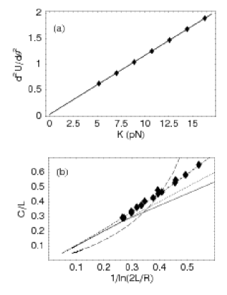
Figure 6: (a) The slope of the torque of a 625$nm$ wire as a function of the elastic constant. The one-elastic constant approximation is used in these simulations. (b) The relationship of capacitance as a function of lengths and radii are explored. Lengths vary from 625$nm$ to 1.25$\mu m$ and radii from 44$nm$ to 198$nm$. The diamonds are the results from our simulations. The exact solution Eq. (39) and the first order approximation, Eq. (40) for the capacitance of a prolate spheroid are the solid and dotted lines respectively. The dashed line is the solution of Brochard and deGennes Brochard and de Gennes (1970). The dash-dot line which traverses through the data is the third order approximation, Eqn. (41), for the capacitance of a prolate spheroid from Jackson.

Having verified the linear relationship in Eqn. (43), we can now turn the situation around and use the known value of $K$ put into the simulation to measure the unknown $C$. This quantity is not experimentally assessable unless an independent measure of the elastic constant $K$ is available. We simulated 15 systems where the length of the wire was varied from $625nm$ to $1.875\mu m$ and the diameter from $22nm$ to $197nm$. This resulted in a minimum aspect ratio of $\sim 3$ to a maximum of $\sim 42$ for the nanowires in our simulations. To avoid finite size effects, we kept the simulation box larger than twice the length of the wire (boxes larger than this gave comparable results). The one elastic constant approximation was used for all simulations, with $K=10.72pN$. Figure 6 (b) shows our results for $C/L$ as a function of $1/\ln(2L/R)$. The dashed line is the incorrect prediction from Brochard and de Gennes which clearly does not predict the capacitance of a prolate spheroid in a correct manner. In Section IV.1 we derived the correct expression for the capacitance of a prolate spheroid, Eqn. (39), as represented by the solid line. The first order approximation is shown by the dotted line. Both of these forms for the capacitance converge for high aspect ratio wires, but fail for low aspect ratio wires. Interestingly, the first order approximation is nearer the simulation results for the wires than the exact solution for the capacitance of a prolate spheroid. For low aspect ratio wires, the expansion of Jackson for a right circular cylinder must be used, and one can see close agreement between this third order approximation and our results. All three theoretical lines (Eqn.(39)-(41)) converge for high aspect ratio wires. For aspect ratios less than $\sim 75$ Eqn. (41) separates from both Eqn. (39) and Eqn. (40) and is obviously the correct expression to use. If one were to use the wires as micro-rheological probes, they would probably need to be a short, low aspect ratio wire (to fit in an in-vivo environment) and similar to the sizes studied within this paper.

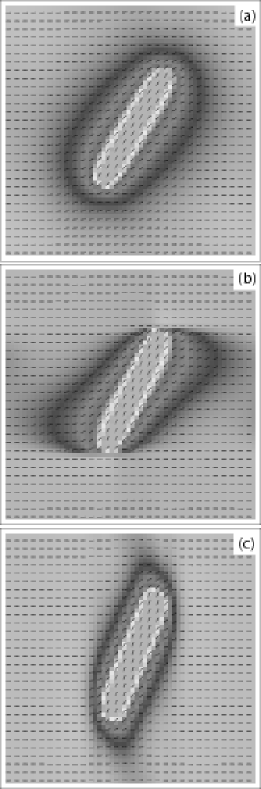
Figure 7: Cross sections of three systems of size $3.75\mu m\times 3.75\mu m\times 3.75\mu m$ with a wire of length $1.875\mu m$ immersed in the center. The wire was rotated from equilibrium to an angle of $\frac{3\pi}{8}$. The shading indicates the inplane nematic angle with the director field of the nematic superimposed. (a) The one elastic constant approximation where $K_{1}=K_{2}=K_{3}$. The director field of the nematic is approximately isotropic in the region surrounding the wire. In (b) $K_{1}<K_{3}$ and in (c) $K_{1}>K_{3}$

In real liquid crystals the elastic constants are not equal (e.g. for 5CB, $K_{1}$ and $K_{3}$ differ by a factor of $\sim 1.6$ Chen et al. (1989)). However, the torque is still observed to be a linear function of $\theta$ in experiments Lapointe et al. (2004, 2005). This brings up the question of which elastic constant, or combination of elastic constants, is measured in these experiments. As the wire rotates through the nematic, one of the modes of deformation, splaying, twisting, or bending, should be favorable for the nematic. The distortion field of the nematic will be greatly affected by the relative differences of the strengths in the various elastic constants. Figure 7 is a density plot of the nematic angle with the director field of the nematic superimposed for three systems with varying elastic constants (A cross section through the center of the cell is shown). In all three panels, the wire was immersed in the center of the nematic as in figure 1, and rotated $\frac{3\pi}{8}$ from equilibrium. In (a) the one elastic constant approximation is used with $K=10.72pN$. The nematic angle forms homeotropic coronas in the region immediately surrounding the wire. In (b) and (c), the one elastic constant approximation is no longer valid as various elastic constants are used. For (b), $K_{1}=15.34pN$, $K_{2}=3.88pN$, and $K_{3}=8.5pN$ and in (c) the values of $K_{1}$ and $K_{3}$ are interchanged. Looking at the density plot of the inplane angle, it is discernible there are clear differences in the distortion pattern the nematic uses to minimize its free energy for these two systems. The splay elastic constant is larger in (b), which explains the distortion field of the nematic exhibiting a higher tendency to bend within the system. Interchanging the elastic constants of splay and bend, as in (c), the distortion field is dominated by splay, as expected.

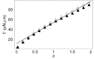
Figure 8: Comparison of the torques of two systems of size $3.75\mu m\times 3.75\mu m\times 3.75\mu m$ with a wire of length $1.875\mu m$. The elastic constants of torque represented by the open diamonds are $K_{1}=15.34pN$, $K_{2}=3.88pN$, and $K_{3}=8.5pN$ and of the filled triangles are the same elastic constants aforementioned with $K_{1}$ and $K_{3}$ interchanged. The solid line is a least squares fit to the data.

Observations of the in-plane nematic angle show discernible differences for the two systems shown Figure 7 (b) and (c). However, the torques of the wires rotating through the two systems are nearly identical, as shown in Figure 8. Even though the elastic constants of splay and bend are interchanged, the torques are approximately equal implying that for Eqn. (43), the same value of $K$ is being measured. Using a least squares fit to the data, the solid line in Figure 8, the slope is $\sim 8pN$ which is approximately the value of the smaller of either splay or bend depending on the system being observed. Thus, experiments will measure the smaller of the splay or bend elastic constant and not some average of the elastic constants as was supposed in Ref. Lapointe et al. (2005). Of course, it may not be known a priori in an experiment which elastic constant is smaller. However, it should be straightforward to observe the birefringence pattern through crossed polarizers and ascertain whether it is more similar to the distortion field shown Fig. 7(b) or (c) and thereby ascertain whether the bend or splay dominates.

V Conclusions

In this paper we present an algorithm to model a moving inclusion in a nematic liquid crystal system. From a knowledge of the capacitance of the ferromagnetic nanowire, it is possible to deduce elastic constants of the liquid crystal from a measurement of the torque. Previously quoted expressions for the capacitance of the wire Brochard and de Gennes (1970) where found to be incorrect and the correct expressions, both for a prolate spheroid and for a right circular cylinder, were given. Most wires used to date have had a very high aspect ratio ($\sim 100$) Lapointe et al. (2005). However, if one were to use the wires as an in-vivo probe of the local elastic properties in, say, a biological environment then much lower aspect wires, or prolate spheroids may be more appropriate. In that case, (i.e. for aspect ratios less than around 75) either the exact expression for the prolate spheroid or the third order expansion by Jackson for the appropriate capacitance should be used.

For realistic systems with multiple elastic constants, we found that the system will tend to trade between splay or bend distortions depending on which one cost less free energy. As a result, the linear elastic response of the nematic to a rotation of the wire is dominated by the smaller of the splay or bend elastic constants. Thus, experiments will typically measure the smaller of $K_{1}$ or $K_{3}$ and not some combination. It should be possible to deduce the elastic constant being measured based on the distortion field of the nematic around the rotated wire, as demonstrated in Fig. 7.

In future works, we will examine the nonlinear response that occurs at wire rotations close to $\pi$ and the dynamical response.