Transport on weighted Networks: when the correlations are independent of the degree

Abstract

Most real-world networks are weighted graphs with the weight of the edges reflecting the relative importance of the connections. In this work, we study non degree dependent correlations between edge weights, generalizing thus the correlations beyond the degree dependent case. We propose a simple method to introduce weight-weight correlations in topologically uncorrelated graphs. This allows us to test different measures to discriminate between the different correlation types and to quantify their intensity. We also discuss here the effect of weight correlations on the transport properties of the networks, showing that positive correlations dramatically improve transport. Finally, we give two examples of real-world networks (social and transport graphs) in which weight-weight correlations are present.

I Introduction

Complex networks have proved to be useful tools to explore natural or man-made phenomena as diverse as the Internet romu-book , human societies newman-review , transport patterns between airports alain04 ; roger05 or even metabolic reactions in the interior of cells almaas04 . The vertices in the networks represent the elements of the system and the edges the interactions between them. The study of the topology of the network provides valuable information on how the basic components interact. While the existence or not of an edge is already informative, in many cases, as those listed above, the interactions can appear on different levels. The bandwidth between two servers on the Internet for instance is not a flat quantity equal for all pairs, it depends on the importance of the servers as well as on the traffic expected. This fact led to the introduction of weighted graphs as a more accurate way to describe real networks yook01 ; newman01 . Weighted graphs are complex networks where the edges have a magnitude associated, a weight. The weight accounts for the quality of a connection. The existence of a distribution of weights dramatically alters transport properties of networks like the geometry of the optimal paths braunstein03 ; goh05 ; wu06 ; chen06 , the spreading of diseases gang05 or the synchronabizability of oscillators zhou05 . Most previous studies have been carried out on networks with uncorrelated weights on neighboring edges (those arriving at the same node) even though most real cases possess correlation. Our aim here is to check how the presence of correlations can influence these results.

There may be several kinds of correlations in random graphs romu06 . Recently, it has been shown that the edge weights in some real-world networks are related to other properties of the graph such as the degree (the number of connections a vertex has) barrat04 ; macdonald05 ; barrat04b . The weights were found to follow, on average, a power law dependence on the degree. Several theoretical mechanisms have been proposed to generate networks of this type models . In this case, a clear correlation is introduced between the weight of neighboring edges but one may wonder whether this is the only possibility for weight correlations. If not, which other structures are possible? How can the correlations be quantitatively characterized? And most importantly, which influence do they have on the transport?

In this work, we address these questions. The organization of the manuscript is the following. In the Section II, we present a model that allows to explore the different configurations for weight correlations independently of other properties of the network. Next, in the Section III, we consider and evaluate different magnitudes to estimate the type and intensity of weight-weight correlations. Section IV includes a study on how the presence of weight correlations affects transport. In Section V two examples of real-world networks showing this type of correlations are discussed: the IMDB actor collaboration network and the traffic network between US airports. And finally, we conclude and summarize in Section VI.

II A simple method to introduce weight-weight correlations

Let us start by defining a mathematical framework for the weight correlations. From the point of view of an edge of weight $w$ with vertices with degree $k$ and $k^{\prime}$ at its extremes, the joint probability that its neighboring edges have a certain weight is given by

$$P_{k\,k^{\prime}}(w,w_{1},\ldots,w_{k-1},w^{\prime}_{1},\ldots,w^{\prime}_{k^{\prime}-1}).$$ (1)

These functions contain all the information about both degree and weight distributions and correlations. However, a situation in which a full hierarchy of such functions were needed to characterize the network would be hard to control from an analytical or numerical point of view. Therefore we will focus here only on the simplest scenario. In the same way the Markovian condition is a simplifying assumption for stochastic processes, we will consider only correlations generated by two-point joint probability functions $P_{k\,k^{\prime}}(w,w^{\prime})$, and, among those, initially only the ones that are degree independent given by functions of the type $P(w,w^{\prime})$.

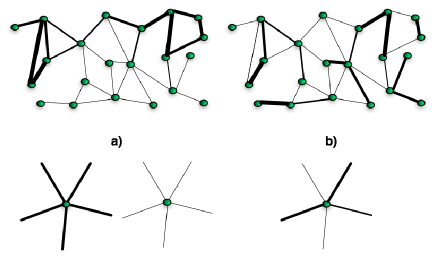
Figure 1: (Color online) Two possible cases in networks with correlations in the link weight: a) positively correlated nets and b) anticorrelated networks. The width of the line of the links represents the value of the weight.

In order to construct weighted networks along these lines, we use the so-called Barabási-Albert (BA) model barabasi99 , where new nodes entering the network connect to old ones with a probability proportional to their degree note1 . The networks generated by this model are scale-free (their degree distribution goes as $P_{k}(k)\sim k^{-3}$), have no degree-degree correlations, and their clustering coefficient (probability of finding triangles) tends to zero when the system size tends to infinity. All this makes them ideal null models to test correlations between edge weights. Once the network is grown, a joint probability distribution for the link weights $P(w,w^{\prime})$ and an algorithm for weight assignation are needed. With the function $P(w,w^{\prime})$ one can calculate the weight distribution $P(w)=\int dw^{\prime}P(w,w^{\prime})$, and the conditional probability of having a weight $w^{\prime}$ provided that a neighboring link has a weight $w$, $P(w^{\prime}|w)=P(w,w^{\prime})/P(w)$. We start by choosing an edge at random and giving it a weight obtained from $P(w)$. Then we move to the nodes at its extremes and assign weights to the neighboring links. To do this, we follow a recursive method: if the edge from which the node is accessed has a weight $w_{0}$, the rest, $w_{1},\ldots,w_{k-1}$, are obtained from the conditional distributions $P(w_{i}|w_{i-1})$. The recursion is necessary to increase the variability in case of anticorrelation (see below). If any of the links, $j$, has already a weight, it remains without change and its value affects the subsequent edges $j+1,\ldots k-1$. We repeat this process until all the edges of the network have a weight assigned note3 .

For $P(w,w^{\prime})$, we have considered different possibilities but here we will focus only on the following three:

$$\begin{array}[]{l}P_{+}(w,w^{\prime})=\frac{X_{+}}{(w+w^{\prime})^{2+\alpha}},\\ \\ P_{U}(w,w^{\prime})=\frac{X_{U}}{(w\,w^{\prime})^{1+\alpha}},\\ \\ P_{-}(w,w^{\prime})=\frac{X_{-}}{(w\,w^{\prime}+1)^{1+\alpha}},\end{array}$$ (2)

where $X_{+}=2^{\alpha}\alpha(1+\alpha)$, $X_{U}=\alpha^{2}$ and $X_{-}=\alpha^{2}/_{2}F_{1}(\alpha,\alpha,1+\alpha,-1)$ are the normalization factors for the distributions on the domain of weights $(1,\infty)$, and ${}_{2}F_{1}()$ is Gauss hyper-geometric function book-hyp . Without losing generality, we have chosen these particular functional forms due to their analytical and numerical tractability. The distributions generated by Eqs. (2) asymptotically decay as $P(w)\sim w^{-1-\alpha}$. The reason to use power-law decaying distributions is that empirical networks commonly show very wide weight distributions that in a first approach can be modeled as power-laws (see Fig. 6 and Refs. almaas04 ; alain04 ; roger05 ; ramasco06a ). We name the functions as $+$ (positively correlated), $-$ (anticorrelated) and U (uncorrelated) because the average weight, $\langle w\rangle(w_{0})=\int dw\,w\,P(w|w_{0})$, obtained with the conditional probabilities from a certain seed $w_{0}$ grows as $\langle w\rangle_{+}(w_{0})=(1+\alpha+w_{0})/\alpha$, decreases as $\langle w\rangle_{-}(w_{0})=(\alpha+1/w_{0})/(\alpha-1)$ and remains constant $\langle w\rangle_{U}=\alpha/(\alpha-1)$, respectively. This means that in $+$ networks the links of each node tend to be relatively uniform in the weights (see Fig. 1a), with separate areas of the graph concentrating the strong or the weak links, while in the negative case links with high and low weights are heavily mixed.

From a numerical point of view, we have checked how the variables to measure vary with the network size $N$. In the following, most results are shown for $N=10^{5}$, which is big enough to avoid significant finite size effects. For each value of the exponent $\alpha$ (from Eqs. (2)) and for each type of correlations, we have averaged over more than $600$ realizations. Note that we use $\alpha$ as a control parameter for the strength of the correlations. For high values of $\alpha$, $P(w)$ decays very fast and the correlations become negligible, all links have almost the same weight. When $\alpha$ decreases however, the higher moments of $P(w)$ diverge and one would expect the correlations to be more prominent.

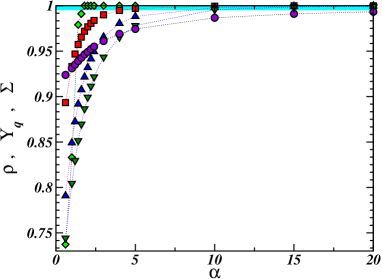
Figure 2: (Color online) The rates $\Sigma_{w}$ (diamonds), $\Upsilon_{q}$, and $\rho$ (circles) for the ”+” distribution model as a function of $\alpha$. The highlighted area encloses the resolution limit of the estimators. The rate $\Upsilon_{q}$ is shown for several values of $q$: $q=2$ (squares), $q=4$ (up triangles) and $q=6$ (down triangles).

III Measures of weight correlations

After a look at the sketch of Fig. 1, the first estimator to consider in order to estimate weight correlations is the standard deviation of the weights of the links arriving at each node. If the weights are relatively homogeneous, the standard deviation will be lower compared with its counterpart in a randomized instance of the graph. The opposite will happen if the correlations are negative as in the case b of Fig. 1. More specifically, for a generic node of the network $i$, $\sigma_{w}(i)$ can be defined as

$$\sigma_{w}^{2}(i)=\sum_{j\in\nu(i)}(w_{ij}-\langle w\rangle_{i})^{2},$$ (3)

where $\nu(i)$ is the set of neighbors of $i$ and $\langle w\rangle_{i}$ is the mean value of the weight of the links arriving at $i$. Once the deviation is calculated for each node, an average can be taken over the full network getting $\langle\sigma_{w}\rangle=(1/N)\sum_{i}\sigma_{w}(i)$. Then to evaluate the effects of weight correlations, it is necessary to compare the value of $\langle\sigma_{w}\rangle_{org}$ obtained for the original network with that measured on uncorrelated graphs. It is, of course, important that the statistical properties of such uncorrelated graphs are as close as possible to those of the original graph. The most accurate procedure consists in disordering only the weights of the links of the original network. To do so, we interchange the weight of each link with that of a randomly selected edge preserving so the weight distribution $P(w)$ and the network topology; $i.e.$, degree distribution, degree-degree correlation, clustering, etc, remain invariant. Once $\langle\sigma_{w}\rangle$ is estimated for the original graph and for an ensemble of weight-reshuffled instances of it, the rate

$$\Sigma_{w}=\frac{\langle\sigma_{w}\rangle_{orig}}{\langle\sigma_{w}\rangle_{rand}}$$ (4)

can be calculated. If $\Sigma_{w}>0$, the weight correlations in the original graph will be as in the case b of Fig 1. If it is identically one, there will be no weight correlations and if $\Sigma_{w}<0$ the correlations will be as in Fig. 1a. The behavior of $\Sigma_{w}$ for the positive and negative models proposed in the previous section is displayed in Fig. 2. The first thing to remark is that indeed $\Sigma_{w}$ can distinguish between the three cases. Moreover, it provides a first method to quantitatively estimate of the intensity of the weight correlations.

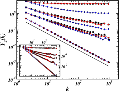
Figure 3: (Color online) Plot of the disparity as a function of the degree, the triplets represent the graphs generated using the ”+” (blue diamonds), the uncorrelated (red squares) and ”-” (black circles) distributions. Each triplet correspond to a different value of $\alpha$, from bottom to top $\alpha=20,1.5,1.2$ and $0.5$. The straight line has slope $-1$ and is meant as a guide to the eye. The triplets have been shifted upwards to facilitate visibility. The inset shows the disparity versus $k$ for the $U$ case and for the values of $\alpha$ from bottom to top $\alpha=20,2,1.5,1.2,1$ and $0.5$.

A similar result can be obtained with a magnitude that was previously discussed in the literature marc03 ; almaas04 . Its name is disparity and was introduced in the context of weighted graphs by Barthélemy et al. as a way to estimate how homogeneous the weights of the links arriving at a vertex are. The generalized disparity of node $i$, $Y_{q}(i)$, is defined as

$$Y_{q}(i)=\frac{\sum_{j\in\nu(i)}w_{ij}^{q}}{s_{i}^{q}},$$ (5)

where $s_{i}$ is the strength of $i$, $s_{i}=\sum_{j\in\nu(i)}w_{ij}$. If all the links of a node have a similar weight, their value will be $w\approx s/k$, and therefore the disparity decays as $Y_{2}(k)\sim 1/k^{q-1}$. On the other hand, if the vertex strength is essentially due to the weight of a single link, $Y_{q}(k)$ will tend to a constant. Typically instead of a generalized $Y_{q}$, most of the works in the literature has focused on $Y_{2}$, for which is commonly reserve the name of disparity. This latter magnitude can be related to $\sigma_{w}$ by the following expression for each node $i$ of the network

$$Y_{2}(i)=\frac{1}{k_{i}}\,\left(1+\frac{\sigma_{w}^{2}(i)}{\langle w\rangle_{i}^{2}}\right),$$ (6)

where $\langle w\rangle_{i}$ is the average weight of the links of $i$ and $k_{i}$ its degree. An important question to mention here is that the profiles of $Y_{q}(k)$ depend on the weight distribution, even for completely uncorrelated graphs. $Y_{q}(i)$ provides information on how different the weights of the links of $i$ are but not on whether that particular configuration is or not a product of randomness or correlations. The variation of $Y_{2}(k)$ with the exponent of the weight distribution $\alpha$ for the uncorrelated $U$-model can be seen in the inset of Figure 3. In the same Figure, we also show the behavior of $Y_{2}(k)$ for the other two models, ”$+$” and ”$-$”, for a few values of the exponent $\alpha$. As before, in order to estimate the importance of the weight correlations, the disparity of the correlated graph has to be compared with that obtained from uncorrelated networks. To express this comparison in a single rate, we can take the average of the disparity over all nodes of the network, $\langle Y_{q}\rangle$, and calculate

$$\Upsilon_{q}=\frac{\langle Y_{q}\rangle_{orig}}{\langle Y_{q}\rangle_{rand}}.$$ (7)

The value of $\Upsilon_{q}$ for the positive model as a function of $\alpha$ is displayed in Fig. 2. This magnitude is also able to discriminate between the different correlations.

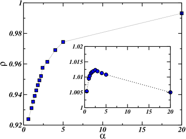
Figure 4: (Color online) In the main plot, the dependence of $\rho$ on the exponent $\alpha$ for the positively correlated graphs generated with the ”+” distribution of Eq. (2). In the inset, the same function but for the graphs of the ”-” distribution.

However, both $\Sigma$ and $\Upsilon_{q}$ have resolution problems. As can be seen in Figure 2 for the positive model, if an area enclosing the numeric error is set immediately below one, the estimators $\Sigma$, $\Upsilon_{q}$ fall in turn relatively fast in that zone. The weights of the links in the ”+” model are continuous variables and therefore they are always correlated. Although, as explained before, for higher values of $\alpha$ the effects of weight correlations can be weaker but still until $\alpha$ is not infinite they are not zero. An ideal estimator should be able to distinguish the $+$ model from a complete random configuration at very high values of $\alpha$. In this context, $\Sigma_{w}$ seems to be the worst estimator. $\Upsilon_{q}$ is better than $\Sigma_{w}$ and improves the higher $q$ becomes. The reason for this behavior is that these magnitudes are not only estimating how wide the spectrum of values of $w$ for a node is, they also supply information on the shape of the distribution of those values. As an example, let us consider a node with $k$ links. The value of $\sigma_{w}$ is higher if $k-1$ of them have weight $a$ and the remaining weight $b$, $\sigma_{w}=|a-b|\,\sqrt{k-1}/\sqrt{k}$, than if the distribution is more symmetric, let us say, with half of them with $w=a$ and the other half with weight $b$, $\sigma_{w}=|a-b|/(2\sqrt{2})$. The goal here is to study how different the amplitude of the weight values is compared with a random configuration of weights, hence the extra information contained in $\sigma_{w}$ or $Y_{q}$ can be neglected. An ideal estimator for weight correlations only needs to consider the interval $|a-b|$. Following this idea, we define the range for a node $i$ as

$$r_{i}=\frac{w_{max}(i)-w_{min}(i)}{w_{max}(i)+w_{min}(i)},$$ (8)

where $w_{max}(i)$ and $w_{min}(i)$ are respectively the maximum and minimum weights of the edges of $i$. The denominator is a normalization factor to keep $r_{i}$ between zero and one. Note that $r$ has a similar behavior to $Y_{q}$ in the limit $q\to\infty$: if all the weights are equal $r=0$, and also $Y_{q}\sim k^{1-q}\to 0$ if $q\to\infty$. On the other hand, if the weight of link dominates the others $r\to 1$, $Y_{q}\to 1$ too if $q\to\infty$. As before, to generate a correlations estimator, the average of $r_{i}$, $\langle r\rangle$, can be taken over all the nodes of the network and contrasted with the equivalent value obtained from a set of weight-reshuffled instances. We will call $\rho$ to the rate between these two quantities,

$$\rho=\langle r\rangle_{orig}/\langle r\rangle_{rand}.$$ (9)

If $\rho<1$, the network displays positive weight correlations. The stronger they are, the smaller $\rho$ becomes. Otherwise, if $\rho>1$, the weights are anticorrelated. $\rho=\Upsilon=\Sigma=1$ is the limit of uncorrelated networks. As can be seen in Fig. 2, $\rho$ is a much more acute estimator of weight correlations than $\Upsilon_{q}$ or $\Sigma$. Hence, from now on we will present our results as function of it. The variation of $\rho$ with $\alpha$ is displayed in Fig. 4 for the ”$+$” and ”$-$” models. The intensity of the correlations for the ”$+$” model grows when $\alpha\to 0$ ($\rho_{+}$ decreases for smaller $\alpha$), while for the negative case $\rho_{-}$ initially grows, peaks around $\alpha\approx 2.5$ and then tends to one again for smaller $\alpha$.

Another question that we are now in position to board is in which way a relation between weight and degree affects the weight-weight correlations. As mentioned in the introduction, networks of this kind may display quite different transport properties from their unweighted counterparts macdonald05 ; luca ; gang05 ; wu06 . Usually, the weights of these networks are obtained by means of a relation of the kind $w_{ij}\sim(k_{i}\,k_{j})^{\delta}$ barrat04 . The result is that provided that the degree is an ”a-priori” characteristic that equally influence all the edges of a vertex, the weight of the links is positively correlated. The networks created in this way show correlations similar to our ”$+$” model (regardless of the sign of the exponent $\delta$) note2 . For instance, for $\delta=\pm 0.5$ the value of $\rho$ is in both cases $\rho\approx 0.832$.

IV Transport properties

Let us focus now on the transport and how it varies with the presence of weight-weight correlations. Several measures have been proposed to study transport wu06 ; transport . In this work we will concentrate on the size and weight of the ”superhighways” as recently introduced by Wu et al. wu06 . If the edges of an uncorrelated network are severed following an increasing order from small to higher weights, the percolation threshold is eventually reached. The remaining connected graph after the process is over, the incipient percolation cluster (IIC) or superhighways, holds most of the traffic of the original network. Regarding this procedure, there are several questions to mention. First, along this work we have assumed that higher weights imply better transport properties. This is also the case for the two empirical examples discussed below; the weights represent number of passengers in one network and number of collaborations done together in the other. However, for some other graphs, the weights can mean higher resistance to transport. And, therefore, the superhighways must be obtained with the same procedure but cutting the links with highest weights first. In such circumstances, the lower the total weight of the superhighway is, the better the transport results.

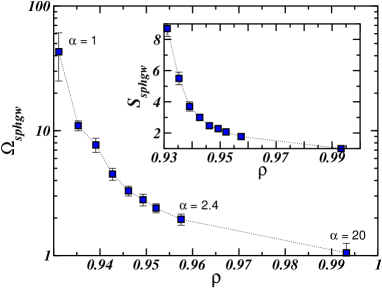
Figure 5: (Color online) Relation between the intensity of the correlations, estimated with $\rho$, and the change in the weight of the superhighways for the positively correlated networks generated with the ”+” model of Eq. (2). The values of $\alpha$ go from $\alpha=1$ for the first point on the left to $\alpha=2.4$ in middle changing regularly by $0.2$ for each point. The last point of the right hand side is for $\alpha=20$.

Another question is that the percolation threshold depends on the topological characteristics of the network. For uncorrelated undirected graphs, it is attained when in the process of severing random links, the rate $\langle k^{2}\rangle/\langle k\rangle$ of the remaining graph approaches two, $\langle k^{2}\rangle/\langle k\rangle=2$ transport . For directed networks or networks with high clustering, the threshold does obey different expressions marian05 . In the next section, we will further discuss this point as well as the numerical determination of the percolation threshold for our two empirical networks.

Finally, it is worthy noting that this method to estimate superhighways cannot be applied directly to networks with weight correlations. If the high weight links are concentrated in some areas of the graph, cutting the weak links is not going to affect those areas. This can change the percolation criterion, i.e. $\langle k^{2}\rangle/\langle k\rangle=2$ cannot be used, although the percolation threshold that depends solely on the topology remains the same as in an uncorrelated graph.

The goal in our case is to compare graphs with and without weight correlations and to quantitatively estimate the effects of these correlations. The method used in practice is to disorder the weights of the links of each correlated network. Then we estimate the superhighways of the randomized graphs and measure how many edges must be cut on average to attain the percolation threshold. Reaching the percolation may have some numerical problems wu07 so the process of reshuffling the weights must be repeated several times. Next, we cut the same number of links in the correlated network (again going from lower to higher values of $w$) and compare the size and the weight of the biggest remaining connected cluster ($W_{sphgw}$) with the average of those found for the randomized graphs. In this way, we obtain

$$\begin{array}[]{l}\Omega_{sphgw}=\frac{W_{sphgw}(orig)}{\langle W_{sphgw}(rand)\rangle},\\ \\ S_{sphgw}=\frac{\mbox{Number nodes in superhighway (orig)}}{\langle\mbox{Number nodes in superhighway (rand)}\rangle}.\end{array}$$ (10)

The results, displayed in Fig. 5, show that, in general, positive correlations play a decisive role on the value of $W_{sphgw}$, increasing it by orders of magnitude. The smaller is $\rho$ respect to the unit, the stronger the effect of the weight correlations on the transport becomes. This phenomenon may be understood by keeping the analogy with the roads: the transport improves if the highways are connected together forming a communication backbone as large as possible. Anticorrelated networks, on the other hand, exhibit smaller superhighways than their randomized counterparts although the effect is subtle.

So far we have discussed models for which the weight correlations are independent of other structural factors. In general, there may be other aspects influencing the transport properties of a graph. If several compete, as it happens in the case $w_{ij}=(k_{i}\,k_{j})^{\delta}$, with $\delta<0$, between the degree and the weight of the connections of a node, the transport capability of the network may suffer. For example, we measure $\Omega_{sphgw}=75(1)$ for networks of size $N=10^{5}$ and $\delta=1/2$, while $\Omega_{sphgw}=0.014(1)$ if $\delta=-1/2$.

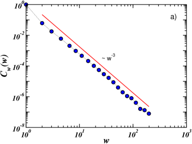
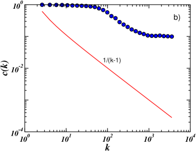
Figure 6: (Color online) In a), cumulative weight distribution $C_{w}=\int_{w}^{\infty}dw\,P(w)$ for IMDB actor collaboration network. In the bottom, in b), the clustering as a function of the degree. The line below corresponds to the function $1/(k-1)$.

V Empirical networks

Finally, we also consider a couple of real-world examples. First the IMDB movie database with $383640$ actors that are connected together whenever they have shared a common movie barabasi99 ; actors . This network is formed by the union of cliques, which means that the number of links is high, $15\,038\,083$ in total. The weight of each link represents the number of times a partnerships has been repeated. Higher values of the weight imply an increased probability of information transfer between two individuals. The cumulative distribution of weights for this network can be seen in Figure 6a. It shows a very wide functional form that can be well represented by a power-law. The presence of weight correlations in collaboration networks have been discussed using a different technique in Ref. ramasco07 . Here we will focus on the results obtained with $\rho$, $\Omega_{sphgw}$ and $S_{sphgw}$.

First of all, it is important to note that collaboration networks typically do not show a relation between the weight of the links defined in this way, or as social closeness newman01 , and the degree of the nodes ramasco07 . Hence the weight correlations, if exist, are not a product of this type of relation. And, indeed, they exist since the actor network presents a value of $\rho=0.268(1)$.

Figure 7: (Color online) Relative size of the giant component as a function of the removal probability $q$ for the actor collaboration networks. In the inset, the same quantity but in log-log and versus $q_{*}-q$. Three values of $q_{*}$ are displayed: $q_{*}=0.9987$ (triangles up), $q_{c}=0.9990$ (circles) and $q_{*}=0.9993$ (triangles down).

The measure of the superhighways in this case poses a certain level of challenge. The actor collaboration network, as many social networks, presents high clustering. The clustering of a node $i$ is defined as

$$c_{i}=\frac{2s_{i}}{k_{i}(k_{i}-1)},$$ (11)

where $s_{i}$ is the number of connections between the neighbors of $i$ and $k_{i}$ stands for its degree. The average over all the nodes of the network with the same degree $k$ can be then taken to obtain $c(k)$, which is depicted in Figure 6b for this network. In the same plot, it is also included the curve $1/(k-1)$. The comparison is necessary because it has been recently shown that the percolation threshold of a graph is highly dependent on the clustering marian05 . In fact, clustered networks can be classified into two major groups: those with weak and those with strong clustering. The difference between the two groups is whether $c(k)$ decays as $1/(k-1)$ (weak clustering) or in a slower way (strong). The actor network clearly falls into this latter group.

For weak clustered networks, it is possible to find a generalization of the percolation threshold condition mentioned in the previous section ($\langle k^{2}\rangle/\langle k\rangle=2$) marian05 . However, as far as we know, nothing similar has been proposed for strong clustered graphs. Therefore, we will be force to use a more pedestrian technique to estimate the percolation threshold of the actor collaboration network. In Figure 7, the behavior of the rate between the size of the giant component $gcc$ and its original value $gcc_{0}$ is displayed as a function of the percentage of links severed $q$. A continuous transition can be observed with this rate as order parameter. Assuming functional form of the type $gcc/gcc_{0}\sim(q_{c}-q)^{\beta}$, we find that the critical point happens at a remotion rate of $q_{c}\approx 0.9990(3)$ (see the Inset of Fig. 7). The point in which the condition $\langle k^{2}\rangle/\langle k\rangle=2$ is fulfilled, for instance, lies in a smaller value $q=0.9976(1)$. Once $q_{c}$ has been measured, we can proceed as in the previous section, cutting a fraction $q_{c}$ of links following an ordered sequence from lower to higher values of the weight and comparing the results with those obtained for a graph in which the weights of the links have been reshuffled. The rates for the total weight of the superhighways for a few values of $q$ are $\Omega_{sphgw}(q=0.9976)=3.2(1)$, $\Omega_{sphgw}(q=0.9987)=17(5)$, and $\Omega_{sphgw}(q_{c}=0.9990)=106(30)$. As can be seen, finding the value of $\Omega_{sphgw}$ requires a fine determination of $q_{c}$. Even so, the high values of this rate gives us a clear feeling of the importance that the weight correlations have on the transport properties of these real world graphs. The values of $S_{sphgw}$ that we find for the same removal rates $q$ are $S_{sphgw}(q=0.9976)=0.62(2)$, $S_{sphgw}(q=0.9987)=3.2(1.5)$, and $S_{sphgw}(q_{c}=0.9990)=20(7)$, respectively.

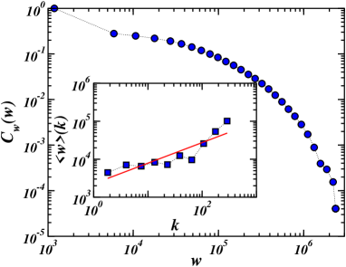
Figure 8: (Color online) In the main plot, the cumulative weight distribution for the US airport traffic network. The average weight of the outgoing connections is displayed in the inset as a function of the out-degree.

The second example is a network composed by $1278$ US airports. A directed edge connects two airports whenever there is a direct flight between them. The weight of the links represent in this case the number of passengers on that traject during $2005$ airports . The cumulative weight distribution of this network is displayed in Figure 8. The weight distribution is in this case also wide, although clearly it does not follow a power-law decay. As can be seen in the Inset of that Figure, the average weight of the outgoing links exhibits a dependence on the out-degree of the nodes, $\langle w_{ij}\rangle\sim(k_{i}k_{j})^{0.42}$. Therefore it is not strange that the value of $\rho$ that we measure, $\rho=0.983(1)$, delates the presence of positive weight correlations. Since the number of passengers in each direction can be different, to calculate the superhighways it is necessary to generalize the concept to directed graphs. This means to study the incipient strongly connected component (SCC) instead of the incipient percolation cluster. Applying the same technique as the one illustrated in Fig. 7, we get a value for the critical removal of $q_{c}=0.988(2)$. The corresponding rate $\Omega_{sphgw}$ is $\Omega_{sphgw}=2.61(7)$.

VI Conclusions

In summary, we have explored how correlations between neighboring edge weights can occur in random networks. The high (low) weights can appear concentrated in certain areas of the graph, a configuration that has a considerable effect on transport properties. To study this phenomenon, we have proposed a simple method to introduce weight correlations in otherwise uncorrelated graphs. These models show that weight correlations can appear independently of any other property of the network, although they could be also coupled to some characteristic of the vertices such as the degree, hidden variables, etc. This method allow us to study, not only qualitatively but also quantitatively, the type and intensity of these correlations. Leading us to test several estimators: $\sigma_{w}$, the generalized disparity and the range $\rho$, being the latter the best of the three.

Once we found a tool to measure the intensity of weight correlations, we have focused on how the transport properties of the network become affected by these correlations. The so called superhighways of our model ”$+$” have been studied as a function of the intensity of weight correlations. The conclusion, that seems to be generalizable to other networks, is that stronger (positive) correlations imply bigger and weightier superhighways, improving thus the performance of the network on transport in orders magnitude.

Finally, we have also considered data from two real-world networks, a collaboration graph and a transportation (airports) network. Both cases present positive weight-weight correlations. The results on their superhighways, $\Omega_{sphgw}$, also prove that weight correlations are without doubt an important factor to take into account in the study of transport on real networks.

Acknowledgments— The authors thank Stefan Boettcher and Eduardo López for useful discussion and comments. Funding from the NSF under grant 0312510 and from Progetto Lagrange was received.

References

- (1) R. Pastor-Satorras and A. Vespignani, Evolution and structure of the Internet: A statistical physics approach, Cambridge University Press, Cambridge (2004).
- (2) M.E.J. Newman, SIAM Review 45, 167 (2003).
- (3) A. Barrat et al., Proc. Natl. Acad. Sci. USA 101, 3747 (2004).
- (4) R. Guimerà et al., Proc. Natl. Acad. Sci. USA 102, 7794 (2005).
- (5) E. Almaas et al., Nature 427, 839 (2004).
- (6) S.H. Yook et al., Phys. Rev. Lett. 86, 5835 (2001).
- (7) M.E.J. Newman, Proc. Natl. Acad. Sci. USA 98, 404 (2001); Phys. Rev. E 64, 016131 and 016132 (2001).
- (8) L.A. Braunstein et al., Phys. Rev. Lett. 91, 168701 (2003).
- (9) K.-I. Goh et al., Phys. Rev. E 72, 017102 (2005).
- (10) Z. Wu et al, Phys. Rev. Lett. 96, 148702 (2006); Phys. Rev. E 74, 056104 (2006).
- (11) Y. Chen et al, Phys. Rev. Lett. 96, 068702 (2006).
- (12) Y. Gang et al., Chinese Phys. Lett. 22 , 510 (2005).
- (13) A.E. Motter, C. Zhou, and J. Kurths, Phys. Rev. E 71, 016116 (2005); Phys. Rev. Lett. 96, 034101 (2006); C. Zhou, and J. Kurths, Phys. Rev. Lett. 96, 164102 (2006).
- (14) M.A. Serrano, M. Boguñá, and R. Pastor-Satorras, cond-mat/0609029 (2006).
- (15) A. Barrat et al., Proc. Natl. Acad. Sci. USA 101, 3747 (2004); Physica A 346, 34 (2005).
- (16) P.J. Macdonald, E. Almaas, and A.-L. Barabási, Europhys. Lett. 72, 308 (2005).
- (17) A. Barrat, M. Barthélemy, and A. Vespignani, Phys. Rev. Lett. 92, 228701 (2004); Phys. Rev. E 70, 066149 (2004).
- (18) S. Dorogovtsev, and J.F.F. Mendes, cond-mat/0408343; K.-I. Goh, B. Kahng, and D. Kim, Phys. Rev. E 72, 017103 (2005); T. Antal, and P.L. Krapivsky, Phys. Rev. E 71, 026103 (2005); G. Bianconi, Europhys. Lett. 71, 1029 (2005).
- (19) A.-L. Barabási and R. Albert, Science 286, 509 (1999).
- (20) We also tested other growth models but the results do not change significantly.
- (21) After the assignation process is over, we have checked that the weights are distributed as for every case.
- (22) N.N. Lebedev, Special functions & their applications, Dover Publications, New York (1972).
- (23) J.J. Ramasco and S. Morris, Phys. Rev. E 73, 016122 (2006).
- (24) M. Barthélemy, B. Gondran, and E. Guichard, Physica A 319, 633 (2003).
- (25) L. Dall’Asta, J. Stat. Mech. P08011 (2005).
- (26) This is not necessarily true for dynamical models models where new edges are introduced at the same time that the weight of the old ones is increased.
- (27) M. Molloy, and B. Reed, Random Struct. Algorithms 6, 161 (1995); E. López et al., Phys. Rev. Lett. 94, 248701 (2005); D.-S. Lee and H. Rieger, Europhys. Lett. 73, 471 (2006);
- (28) M.A. Serrano and M. Boguña, Phys. Rev. Lett. 97, 088701 (2006); Phys. Rev. E 74, 056114 (2006);Phys. Rev. E 74, 056115 (2006); Phys. Rev. E 72, 016106 (2005).
- (29) Z. wu et al.,condmat/0705.1547.
- (30) Data available at http://www.nd.edu/networks/database/index.html.
- (31) J.J. Ramasco, Eur. Phys. J. ST 143, 47 (2007).
- (32) Databases at http://www.transtats.bts.gov/.