Phase diagram of vortex matter in layered superconductors with random point pinning

Abstract

We study the phase diagram of the superconducting vortex system in layered high-temperature superconductors in the presence of a magnetic field perpendicular to the layers and of random atomic scale point pinning centers. We consider the highly anisotropic limit where the pancake vortices on different layer are coupled only by their electromagnetic interaction. The free energy of the vortex system is then represented as a Ramakrishnan-Yussouff free energy functional of the time averaged vortex density. We numerically minimize this functional and examine the properties of the resulting phases. We find that, in the temperature ($T$) – pinning strength ($s$) plane at constant magnetic induction, the equilibrium phase at low $T$ and $s$ is a Bragg glass. As one increases $s$ or $T$ a first order phase transition occurs to another phase that we characterize as a pinned vortex liquid. The weakly pinned vortex liquid obtained for high $T$ and small $s$ smoothly crosses over to the strongly pinned vortex liquid as $T$ is decreased or $s$ increased – we do not find evidence for the existence, in thermodynamic equilibrium, of a distinct vortex glass phase in the range of pinning parameters considered here. We present results for the density correlation functions, the density and defect distributions, and the local field distribution accessible via $\mu$SR experiments. These results are compared with those of existing theoretical, numerical and experimental studies.

I Introduction

Equilibrium and transport properties of the mixed phase of highly anisotropic, layered, high-temperature superconductors (HTSCs) in the presence of various kinds of pinning have been studied extensively for over one decade.review Random pinning destroys the long-range translational order of the Abrikosov lattice and leads to a variety of low-temperature glassy phases. In systems with random point pinning, the existence of a topologically ordered Bragg glass (BrG) phase with quasi-long-range translational order at low temperatures, low fields and weak pinning is now well-established both theoretically natt ; giamarchi and experimentallyklein . The BrG is expected to melt into a vortex liquid (VL) via a first-order transition as the temperature is increased. The possibility of occurrence of an amorphous vortex glass (VG) phase (with nonlinear voltage-current characteristics and vanishing resistance in the zero-current limit) at low temperatures in systems with strong pinning (or at high magnetic fields where the effects of pinning disorder are enhanced) was suggested several years ago mpa ; ffh . However, in spite of extensive investigation over almost twenty years, whether a true VG phase (that is, an amorphous glassy phase thermodynamically distinct from the high-temperature VL) exists in systems with uncorrelated point pinning remains controversial.

Evidence for the theoretically expected scaling behavior of the current-voltage characteristics near a continuous VL–VG transition was obtained in several early experiments.vglexp The validity of the conclusions drawn from these experiments has been questioned in latter studies,lobb although a recent experimental studyzeldov has presented intriguing thermodynamic evidence for the existence of a VG phase. Numerical studiesbokil of a “gauge-glass” model believed to be in the same universality class as vortex systems with random point pinning suggest that a finite-temperature VG phase does not exist in three dimensions if electromagnetic screening of the interaction between vortices is taken into account. Other numerical studiesolsson ; lidmar ; nh of models in which the interaction between vortices is not screened indicate the presence of a thermodynamically stable VG phase at low temperatures if the pinning is strong. One of thesenh also presents evidence for the existence of a “vortex slush” phase with short-range translational order (i.e. a translational correlation length significantly longer than that in the VL phase) but no long-range phase coherence. However, the existence of this phase has been questioned in later work.teitel A variety of interesting “glassy” behavior has been experimentally observed banerjee near the first-order melting transition of the BrG phase of superconductors (both conventional and HTSCs) with point pinning. It is possible thatbanerjee ; gautam these observations can be understood by assuming that the melting of the BrG phase occurs in two steps: the BrG first transforms into a “multidomain” glassy phase that then melts into the usual VL at a slightly higher temperature.

It is clear from this brief summary of the many existing theoretical and experimental results that several important issues about the structure and phase behavior of vortex matter in the presence of random point pinning are still unresolved.

In this paper we present the results of a numerical study of the structural and thermodynamic properties of the system of vortices in a highly anisotropic layered superconductor in the presence of random point pinning. The magnetic field is perpendicular to the superconducting layers and the vortex lines can then be considered as stacks of pancake vortices residing on the layers. These pancake vortices constitute a system of point-like objects that interact among themselves and also with an “external” potential arising from a small concentration of randomly placed pinning centers (atomic scale defects). The positions of these defects on different layers are assumed to be completely uncorrelated. In this highly anisotropic case, the Josephson coupling between layers is vanishingly small, and pancake vortices on different layers are coupled only through the electromagnetic interaction. Under these circumstances, one can use (as in our recent studies prbv ; prbd of vortex systems in the presence of columnar pinning) a spatially discretized version of the Ramakrishnan-Yussouff free energy functional ry for a system of pancake vortices. In this formalism, the free energy of the system is expressed as a functional of the time-averaged local density of vortices. The different local minima of this functional can then be found by starting the numerical minimization process with appropriate initial conditions. These local minima, whose density configurations are obtained in our calculations, can then be identified with different phases of the system in our mean field description: the nature of the phase corresponding to a particular local minimum is determined from a detailed analysis of the density distribution and the correlation functions at that minimum. A first-order transition between two phases, represented by two different locally stable minima of the free energy functional, is signaled by a crossing of the free energies of these minima as some control parameter (e.g. the temperature) is varied.

Using this method, we have analyzed the phase diagram of the system as a function of temperature and pinning strength for a fixed value of the magnetic induction, which determines the areal density of pancake vortices. For low temperatures and relatively small values of the pinning strength, we find a nearly crystalline minimum that exhibits all the properties expected for a BrG phase (the “BrG minimum”). This BrG phase is the thermodynamically stable one (has the lowest free energy) if the temperature is sufficiently small and the pinning sufficiently weak. It becomes unstable very soon after either of these parameters is increased beyond the region where this is the equilibrium phase. We find another local minimum at which the density distribution in each layer is strongly disordered (amorphous) and the densities in different layers are weakly correlated. This minimum is at least locally stable for the range of temperature and pinning strength we have considered. If the temperature is high and the pinning strength low, then the density distribution at this minimum is weakly inhomogeneous, showing the characteristics expected for a weakly pinned VL. As the temperature is reduced, or the pinning strength is increased, this minimum evolves continuously into a state with strong inhomogeneity in the distribution of the time-averaged local density. This state represents a system of pancake vortices strongly localized at random positions because of the random pinning potential. This state exhibits characteristics of a glass, but we prefer to call it a strongly pinned VL because it is continuously connected to the weakly pinned VL found for high temperatures and weak pinning – we do not find any indication of a phase transition between the liquid-like and glass-like states.

As the temperature is increased at a fixed, relatively small value of the pinning strength, or the pinning strength is increased at a sufficiently low temperature, the free energy of the BrG minimum crosses that of the VL minimum, signaling a first-order phase transition from the BrG to the pinned VL phase. For very weak pinning, the temperature at which this transition occurs is nearly independent of the pinning strength: it is very close to the melting temperature of the unpinned vortex lattice. As the pinning strength is increased, the transition temperature decreases and eventually, the transition line in the temperature – pinning strength plane exhibits a trend towards becoming parallel to the temperature axis. Thus, the BrG phase is thermodynamically stable only if the pinning strength is lower than a critical value. The shape of the boundary of the BrG phase is similar to that found in existing numerical simulation studies.nh ; teitel2 As mentioned above, the local minimum corresponding to the VL phase remains locally stable as the transition line to the BrG phase is crossed either by reducing the temperature or by decreasing the pinning strength. On the other hand, the BrG minimum becomes unstable (and the minimization converges to a minimum of the VL type) as the temperature or the pinning strength is increased slightly beyond the point at which the transition to the VL phase occurs. This behavior is consistent with experimental results andrei that indicate that the superheated BrG phase in ${\rm NbSe_{2}}$ exhibits a spinodal instability, whereas there is no limit of metastability of the supercooled disordered state. We have also carried out a careful search for the presence of local minima of the free energy that may correspond to the “vortex slush” phase nh or the polycrystalline “domain glass” phase gautam predicted in some earlier studies. As we will explain below, we did not find any equilibrium free energy minimum that could be interpreted as either one of these phases although we have found some indications that they may occur under nonequilibrium conditions.

We have used our results for the vortex density distribution at the free energy minima to calculate the distribution of the local (microscopic) magnetic induction in the sample. This is important because the distribution of the local magnetic induction is measured in muon spin rotation ($\mu$SR) experiments, and phase transitions in the vortex system give rise to characteristic changes in the width and shape of this distribution. Thus, $\mu$SR experiments have been widely used musrrev to study phase transitions in the mixed state of HTSCs and conventional type-II superconductors. Our results show a relatively broad and asymmetric distribution of the microscopic magnetic induction in the BrG phase, and a narrow and much more symmetric distribution in the VL phase. These features are in good agreement with available $\mu$SR data.

The rest of this paper is organized as follows. In section II, we define the model we consider and describe the numerical method used in our study. The results of our calculations are described in detail and compared with existing experimental and numerical results in section III. Section IV contains a summary of our main results and a few concluding remarks.

II Model and Methods

We consider a layered superconductor in a magnetic field perpendicular to the layers. We assume that the material is strongly anisotropic so that the Josephson coupling between layers is vanishingly small. The pancake vortices on different layers are then coupled only through their electromagnetic interaction. In this limit, vortices in the same layer repel each other with a potential logarithmic in their separation, while there is a much weaker attractive interaction between vortices on different layers which falls off exponentially with layer separation and varies logarithmically with the separation in the layer plane. This model for the vortex system was used in our earlier studies prbv ; prbd of the effects of columnar pinning. As discussed in detail in Ref. prbv, , many theoretical and experimental studies indicate that this model is appropriate for describing the properties of vortex matter in highly anisotropic materials such as BSCCO (${\rm Bi_{2}Sr_{2}CaCu_{2}O_{8+x}}$) in a large region of the field–temperature plane, although this conclusion has been questioned in a recent theoretical analysis roz .

The free energy functional of such a system of pancake vortices lying on the superconducting layers and interacting with a time-independent pinning potential can be written in the form:

$$F[\rho]=F_{RY}[\rho]+F_{p}[\rho]$$ (1)

The first term in the right side of Eq. (1) is the free energy of the vortex system in the absence of pinning, while the second includes the pinning effects. The first term is of the Ramakrishnan-Yussouff form ry :

$$\beta F_{RY}[\rho]=\sum_{n}\int{d{\bf r}\{\rho_{n}({\bf r})\ln(\rho_{n}({\bf r})/\rho_{0})-\delta\rho_{n}({\bf r})\}}-(1/2)\sum_{m}\sum_{n}\int{d{\bf r}\int{d{\bf r}^{\prime}C_{mn}({|\bf r}-{\bf r^{\prime}|})\delta\rho_{m}({\bf r})\delta\rho_{n}({\bf r}^{\prime})}},$$ (2)

where $\beta$ is the inverse temperature. We have defined $\delta\rho_{n}({\bf r})\equiv\rho_{n}({\bf r})-\rho_{0}$ as the deviation of ${\rho_{n}(\bf r})$, the time-averaged areal density of pancake vortices at point $\bf r$ on layer $n$, from $\rho_{0}$, the density of the uniform liquid ($\rho_{0}=B/\Phi_{0}$ where $B$ is the magnetic induction and $\Phi_{0}$ is the flux quantum) and we have taken our zero of the free energy at its uniform liquid value. The integrations are two-dimensional and the sums are over all layers. The function $C_{mn}(r)$, which depends on the layer separation $|m-n|$ and the separation $r$ in the layer plane, is the direct pair correlation function of the layered vortex liquid hansen at density $\rho_{0}$. This static correlation function contains all the required information about the interactions in the system. We have used here the $C_{mn}(r)$ obtained from a calculation menon1 via the hypernetted chain approximation hansen for parameter values appropriate for BSCCO, as in Ref. prbd, : $d=15\AA$ for the interlayer distance, and a two-fluid form for the temperature dependence of the penetration depth $\lambda(T)$ with $\lambda(0)=1500\AA$.

The second term in Eq.(1) represents the effects of pinning and can be written as

$$F_{p}[\rho]=\sum_{n}\int{d{\bf r}V^{p}_{n}({\bf r})[\rho_{n}({\bf r})-\rho_{0}]},$$ (3)

where $V^{p}_{n}({\bf r})$ is the pinning potential at point ${\bf r}$ on layer $n$. The pinning potential is assumed to be produced by random atomic scale point defects. The positions of the defects on different layers are assumed to be completely uncorrelated. Each defect is assumed to produce a pinning potential of depth $v_{0}$ and having a short range which we will take (see below) as of the order of the spacing $h$ of the computational mesh in our numerical calculation. A randomly chosen small fraction, $c$, of the unit cells of the underlying crystal lattice, taken to be a square lattice with spacing $d_{0}=4\AA$, are assumed to be occupied by pinning defects.

If the time averaged vortex density is the same on all layers (as would be the case for columnar pins perpendicular to the layers), the free energy could be written in an effectively two-dimensional form prbv ; prbd with the quantity $\tilde{C}(r)\equiv\sum_{n}C_{mn}(r)$ playing the role of the two-dimensional direct correlation function. But in the present case, with a pinning potential that varies from one layer to another, the full three dimensional problem has to be considered. The problem is therefore computationally much more demanding. To numerically minimize the free energy of the system, we discretize the density variable by introducing a layered triangular computational lattice containing $N^{2}$ sites on each layer. The total number of computational mesh points is thus $N^{2}N_{L}$ where $N_{L}$ is the number of layers considered. We use periodic boundary conditions in all three directions. On the sites of this lattice we define discretized density variables $\rho_{n,i}\equiv\rho_{n}({\bf r}_{i})A_{0}$, where $\rho_{n}({\bf r}_{i})$ is the density at mesh point $i$ on layer $n$ and $A_{0}$ the area of the unit cell of the in-plane computational lattice. A numerical procedure developed earlierprbv ; cdo is used to find local minima of the free energy written as a function of the variables $\{\rho_{n,i}\}$.

We use the quantity $a_{0}$ defined by $\pi\rho_{0}a_{0}^{2}\equiv 1$ as our unit of length. The spacing of the triangular computational lattice is taken to be $h=a/16$ where $a=1.998a_{0}$ is the equilibrium lattice constant prbv of the Abrikosov vortex lattice in the absence of pinning in the temperature range considered (see below) which is chiefly determined by the melting temperature of the unpinned vortex lattice, namely $T_{m}^{0}\simeq$ 18.4K prbv at the field considered in this work ($B$ = 0.2T). The total number of defects on each layer of our sample is given by $N_{d}=\sqrt{3}(Nh)^{2}c/(2d_{0}^{2})$. In our discretized system, the values of the pinning potential $V_{n,i}$ associated with mesh point $i$ on the $n$th layer are determined in the following way: for each layer, we generate $N_{d}$ points distributed randomly and uniformly over the area of the layer. The potential $V_{n,i}$ is then taken to be $v_{0}(m_{n,i}-N_{d}/N^{2})$ where $m_{n,i}$ is the number of such point in the $i$th computational cell on layer $n$, and $N_{d}/N^{2}$ is the average value of $m_{n,i}$. We take $c$ to be 0.01 (1%) and measure $v_{0}$ in units of $k_{B}$, the Boltzmann constant, so that the parameter $s\equiv v_{0}/k_{B}$ (with values given in Kelvins) measures the strength of the pinning potential. With this parametrization, we have $\langle V_{n,i}\rangle=0$, and $\langle\beta V_{n,i}\beta V_{n^{\prime},j}\rangle=2.68(s/T)^{2}\delta_{nn^{\prime}}\delta_{ij}$ where $T$ is the temperature and the angular brackets denote the average over the random configuration of defects.

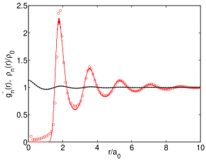
Figure 1: (Color online). Plots of the local density $\rho_{n}(r)$, normalized by the average density $\rho_{0}$, for $n=0$ ((red) circles) and $n=1$ ((black) dots), as functions of $r/a_{0}$. Here, $n$ is the layer separation and $r$ is the in-plane distance from a single strong pinning center that traps a pancake vortex. The results for the pair distribution function ${g^{\prime}}_{n}(r)$ are also shown for comparison ((red) dashed line: $n=0$; (black) solid line: $n=1$). These results are for the vortex liquid state at temperature $T$ = 20K and field $B$ = 0.2T.

To test the numerical method described above, we carried out a minimization of the free energy for a system in which a single strong pinning center was placed on one of the layers. The depth and the range of the potential produced by the pinning center were chosen (as in Ref. prbv, , see Fig. 3 in that work) so as to ensure that it traps a single vortex at the temperature $T$ = 20K (the unpinned vortex system is in the liquid state at this temperature prbv ). According to a well-known result in liquid state theory hansen , the time-averaged local density $\rho_{n}(r)$ outside the range of the potential produced by the pinning center (here, $n$ denotes the separation from the layer in which the pinning center is located, and $r$ is the in-plane distance from the position of the pinning center) should be equal to $\rho_{0}{g^{\prime}}_{n}(r)$ where ${g^{\prime}}_{n}(r)$ is the pair distribution function of the unpinned vortex liquid, which can be obtained from the direct pair correlation function $C_{n}(r)$ used as input in our calculations. The results for $\rho_{n}(r)/\rho_{0}$, obtained from a numerical minimization of the discretized free energy (with $N=128$ and $N_{L}=32$) are shown in Fig.1 for $n$ = 0 and $n$ = 1 (for $n=0$, the results for $\rho_{n}(r)/\rho_{0}$ are shown for values of $r$ outside the range of the potential produced by the pinning center at $r=0$). The plots also show the values of ${g^{\prime}}_{n}(r)$ obtained from the $C_{n}(r)$ used as input. The agreement between the two sets of results is quite good (the small differences may be attributed to the fact that the peak of the local density at the pinning center at $r=0$ is not a $\delta$-function). These results confirm that the numerical method used in our calculations correctly reproduces the strong intra-layer correlations, as well as the much weaker inter-layer correlations of local density of the system of pancake vortices.

III Results

We now present our results. The values of the temperature $T$ and pin strength parameter $s$ are indicated in each case. The field is always $B=0.2T$. The number of layers is $N_{L}=128$ and the transverse computational lattice size $N=256$. With the value of the computational lattice constant $h$ being $h=a/16$ where $a=1.988a_{0}$ isprbv the equilibrium lattice constant of the vortex lattice, the number of pancake vortices in each layer is $N_{v}=256$. The absence of finite size effects has been verified by checking that these larger-size results are nearly identical to those obtained for smaller systems. Results have been obtained for five random pin configurations and averaged over this number (except as indicated) whenever appropriate. This is a sufficient number as we find that the differences between results for different pin configurations of the same strength and concentration are negligible for the quantities of interest.

We use several kinds of initial conditions to start the minimization process. In the first kind, we start with uniform “liquid-like” conditions, with the variables $\rho_{n,i}$ all equal to their average value. The second kind is “crystal-like”: the initial $\rho_{n,i}$ variables are obtained, for a given random pin configuration, by minimizing the pinning energy of the equilibrium crystalline configuration in the absence of pinningprbv for the value of $B$ used here, with respect to the symmetry operations of the computational lattice. Thirdly, once a local minimum configuration has been obtained from the minimization procedure for certain values of $s$ and $T$, that configuration is used as the initial condition for a nearby value of either one of these variables. The first kind of initial conditions leads, after minimization, to free energy minima which are, as we shall see below, disordered in a liquid-like or glass-like way. The second kind yields BrG states, provided however that the values of $T$ or $s$ are not too high: if they are, the crystal-like BrG state is not stable and those initial conditions lead eventually to a disordered state. The third kind leads to a state of the same general kind as the initial one, except when an instability boundary is crossed.

III.1 Structure of free energy minima

¿From the set of values for the $\rho_{n,i}$ at each local minimum, the nature of that minimum can be ascertained by evaluating the appropriate correlation functions and also by direct visualization of either the density variables or of the “vortex lattice” formed by the locations of the peaks of the local density.

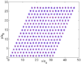
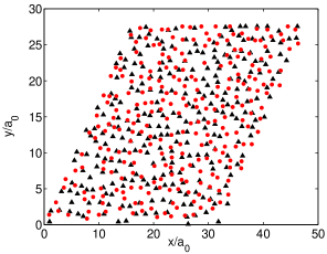
Figure 2: (Color online). Visualization of density structures at different kinds of free energy minima. The first two panels correspond to an ordered minimum. In the first, the (blue) dots indicate, for each of the 128 layers present, the positions of pancake vortices in that layer. The (red) filled circles denote the average positions of “vortex lines” obtained by connecting adjacent vortices on neighboring layers. In the second panel, the (red) full circles have the same meaning and the (black) triangles represent the vortex position in a randomly chosen layer. In the third panel, the (red) full circles and the (black) triangles represent the positions of pancake vortices on two adjacent layers in a disordered minimum. In all cases $T=17.0K$ and $s=10.0K$.

To visualize the vortex lattice, the local peak densities are extracted from the set of $\rho_{n,i}$ values by defining site $i$ in layer $n$ to be a peak location when it corresponds to a local maximum of the $\rho_{n,i}$ such that the value $\rho_{n,i}$ exceeds that of any $\rho_{n,j}$ in the same plane and within a radius $a/2$ from $i$. The positions of such “vortex sites” in each layer can then be plotted. An example is given in Fig. 2. The results there are all at $s=10.0K$ and $T=17.0K$. In the first panel, a small (blue) dot denotes the position of a vortex site at any one of the 128 layers. The results plotted correspond to a state obtained starting with “crystal-like” initial conditions, as explained above. The vortex positions are clearly clustered into well-defined groups that form a triangular pattern. For such minima, we can define “vortex lines” by joining the vortex positions in each group on different layers. The (red) filled circles in the first panel indicate the average positions of these vortex lines. These average positions form a slightly distorted triangular lattice, with considerable variation, however, from layer to layer. The typical size of the clusters of (blue) dots represents the degree of transverse layer-to-layer wandering of the vortex lines. In the second panel, the same point is emphasized by displaying again the average positions as (red) filled circles, and the vortex positions at a randomly chosen layer as triangles: the degree of crystalline order in the average positions of the vortex lines is higher than that in the vortex positions on a typical layer – the random transverse displacements of the vortex positions on different layers from the ideal triangular lattice partly cancel out in the calculation of the average positions of the vortex lines. From these results and other evidence discussed below, we identify minima of this kind as representing the BrG phase.

If one plots the vortex positions as in the first panel of Fig. 2 for a minimum obtained from liquid-like initial conditions at the same $T$ and $s$, one obtains a nearly uniform space-filling plot: the positions of the pancake vortices on different layers are nearly uncorrelated at this minimum. This difference between the two kinds of local free energy minima is emphasized in the third panel of Fig. 2 where the vortex positions in two neighboring layers are plotted for a disordered minimum obtained for the same pin configuration, $T$, and $s$ as those for the plots in the first two panels. Disordered local minima of this kind are identified below as representing the VL phase.

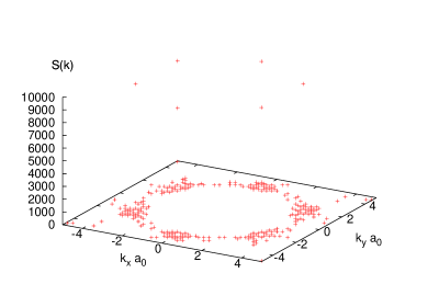
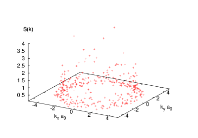
Figure 3: (color online).The static structure factor as defined in Eq. (4) plotted versus the two dimensional wavevector (in units of $a_{0}^{-1}$) at $T=17.0K$ and $s=10.0K$ for the equilibrium ordered state under these conditions (first panel) and for the metastable disordered state (second panel).

It is very useful to discuss also the difference between ordered and disordered states in terms of correlation functions. We do this in the next two figures. Consider first Fig. 3. There we plot the “two-dimensional” static structure factor $S({\bf k})$ defined as:

$$S({\bf k})=|\rho({\bf k},k_{z}=0)|^{2}/(N_{v}N_{L})$$ (4)

where $\rho({\bf k},k_{z})$ is the discrete Fourier transform of the $\{\rho_{n,i}\}$ in terms of the wavevector $({\bf k},k_{z})$ (the $z$-axis is normal to the layers). In the figure $T=17.0K$ and $s=10.0K$. In the first panel $S({\bf k})$ is plotted for the ordered state (which is, as we shall see, the equilibrium one in this case) while in the other panel the same quantity is plotted for the disordered state obtained from uniform initial conditions, which is locally stable at these values of $s$ and $T$. The difference between the two states can be readily seen: note the large difference between the vertical scales in the two plots and the Bragg-like peaks in the ordered case.

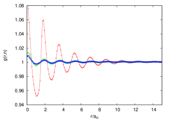
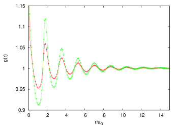
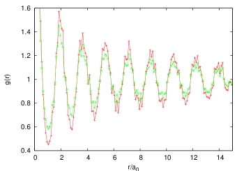
Figure 4: (Color online) Real-space angularly averaged correlation functions (see text) plotted versus two-dimensional dimensionless in-plane distance at $T=17.0K$. The first panel displays (top to bottom curves at small $r$) $g(r,n)$ for $n=0$ (red), $n=1$ (green), and $n=10$ (blue) at $s=10.0K$, in the disordered state. The second and third panels show $g(r)\equiv g(r,n=0)$ for the disordered and ordered states, respectively, at $s=10.0K$ and $s=12.0K$, with the paler (green) curve corresponding to the higher $s$.

Alternatively, one can look at real-space correlation functions obtained from the discrete Fourier transform of $S({\bf k},k_{z})$. We define $g(r,n)$ as the angularly averaged correlation of the time-averaged local densities at two points separated by $n$ layers and in-plane distance $r$. The same-plane correlation function is $g(r)\equiv g(r,n=0)$. For $n\neq 0$, $g(r,n)$ represents correlations between the vortex densities in different planes. We normalize $g(r,n)$ by $\rho_{0}^{2}$, so that it approaches unity at large values of $r$ for all $n$. These correlation functions are different from the pair distribution function ${g^{\prime}}_{n}(r)$ shown in Fig. 1: the $g(r,n)$ represent correlations of time-averaged local densities, whereas ${g^{\prime}}_{n}(r)$ are the equal-time correlation functions of the instantaneous local density. In particular, $g(r,n)$ equals exactly unity for all $n$ and $r$ for a homogeneous vortex liquid in the absence of any pinning, while ${g^{\prime}}_{n}(r)$ for a homogeneous liquid shows oscillations (seen in Fig. 1) that reflect the short-range correlations present in a liquid. In the presence of a pinning potential that makes the time-averaged local density in the liquid phase inhomogeneous, the correlation function $g(r,n)$ represents the spatial correlations of this pinning-induced inhomogeneity.

Results for $g(r,n)$ are presented in Fig. 4. In the first panel $g(r)$, $g(r,1)$ and $g(r,10)$ at $T=17.0$ and $s=10.0K$ for the liquid-like metastable state are shown. The decay of the correlations with $n$ is clear: the vortex densities on different layers are only weakly correlated in the liquid-like phase, in agreement with the results shown in the third panel of Fig. 2. The corresponding plot for the ordered state at the same values of $T$ and $s$ (not displayed) would show no decay with $n$ except at very small values of $n$, indicating that the vortices on different layers are close to registry in this state. In particular, $g(r=0,n)$ is found to be essentially independent of $n$ for $3<n\lesssim N_{L}/2$ in the ordered phase, showing absolutely no sign of decay for large values of $n$. In the other two panels, the variation of $g(r)$ with $s$ is shown for both the disordered and the ordered states and two values of $s$. The two cases are again in stark contrast. For the disordered, liquid-like minimum (second panel), the amplitude of the damped oscillations of $g(r)$ is much smaller than that for the ordered, crystal-like minimum (third panel). The amplitude of these oscillations increases with $s$ for the liquid-like minimum because the pinning-induced inhomogeneity in the local density increases as the pinning gets stronger, whereas for $g(r)$ in the ordered minimum, this amplitude decreases as $s$ is increased, reflecting that stronger pinning leads to larger distortions of the crystalline structure. One could similarly plot the variation of $g(r)$ with temperature: in this case the peak heights decrease as $T$ increases. All these features of $g(r,n)$ for the liquid-like state are very similar to those found in an analytic study gautamprl of the effects of pinning disorder on the correlations of a layered vortex liquid.

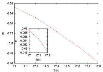
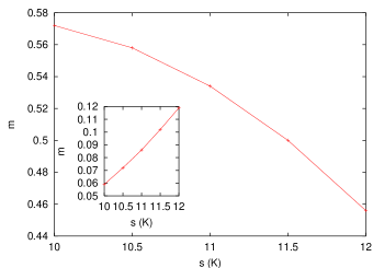
Figure 5: (Color online).First panel: The order parameter $m$, as defined in the text, plotted versus temperature at constant $s=10.0K$ for the ordered state (main plot) and the disordered state (inset). Second panel: The same quantity plotted versus pin strength $s$ at constant $T=17.0K$ for the ordered state (main plot) and the disordered state (inset). The solid lines are guides to the eye.

From the correlation functions, an appropriate order parameter can be extracted. A convenient definition is $m\equiv g(r_{m})-1$ where $r_{m}$ is the first nonzero value of $r$ for which $g(r)$ has a peak. An alternative definition prbd in terms of $S({\bf k},k_{z}=0)$ yields very similar results. In the first panel of Fig. 5, this quantity is plotted as a function of the temperature at constant $s=10.0K$ for both the ordered and (inset) the disordered state. It is, as it should be, much larger in the former case and it decreases with increasing $T$ for both states. As we shall see below, the transition temperature at this value of $s$ is near $T=17.44K$. In the second panel of Fig. 5, $m$ is plotted versus $s$ at constant $T=17.0K$ for the same two cases. The transition as $s$ is increased at this $T$ occurs at $s=11.1K$. We see that $m$ now increases with $s$ in the disordered state while remaining much smaller than its values in the ordered state. In the ordered state, $m$ decreases with $s$, as expected.

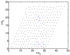
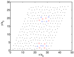
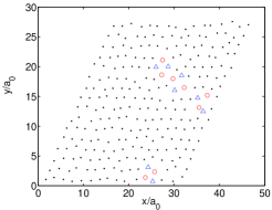
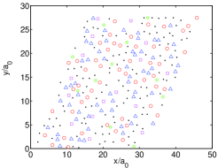
Figure 6: (Color online) Voronoi plots of the vortex lattice. The (black) dots denote ordinary sites with six neighbors, the (red) circles sites with seven neighbors and the (blue) triangles sites with five neighbors. The first three panels are for the ordered state with $s=10.0K$, $T=17.0K$ (top left panel), $s=10.0K$, $T=17.4K$ (top right panel), and $s=12.0K$, $T=17.0K$ (bottom left panel). The last panel is for the disordered state at $s=10.0K$, $T=17.6K$. The (green) filled circles and (magenta) squares in this plot represent sites with eight and four neighbors, respectively.

It is also useful to visualize the defect structure of the phases by means of Voronoi plots of the vortex lattice. In these plots the number of neighbors of each vortex lattice site in a given layer is found via a Wigner-Seitz construction. One then plots with different symbols the lattice points having six neighbors (this would be all the sites for a defect-free lattice) and those having e.g. seven or five neighbors (which correspond to single disclinations: neighboring pairs of disclinations of opposite sign correspond to dislocations). The results are shown in Fig. 6. The first three panels are for the ordered state, at $s=10.0K$, $T=17.0K$ (top left panel), $s=10.0K$, $T=17.4K$ (top right panel), and $s=12.0K$, $T=17.0K$ (bottom left panel). The system is deep in the ordered phase for the first set of values of $s$, $T$, while the other two sets represent points close to the phase boundary (see below) between the ordered and disordered phases. In each case, the defect structure in the layer with the largest number of defects is plotted. One can see a few dislocations in each of the three plots, but these dislocations occur in tightly bound clusters with zero net Burgers vector. The number of defects is small and increases only weakly with $T$ for fixed $s$, and with $s$ if $T$ is fixed. One clearly has a rather well ordered crystal-like structure even for values of $s$ and $T$ close to the phase boundary. A feature to note in these plots is that all these structures are single-domain: domain boundaries which appear in Voronoi plotsprbd as lines of defect pairs are clearly absent. By contrast, the last panel in this figure, which depicts the disordered state obtained for $s=10.0K$ and $T=17.6K$ (the disordered state is the equilibrium one for these parameter values, see below), shows a very large number of randomly distributed defects. The structure of this state may be classified as amorphous – there is no indication of the presence of grain boundaries separating crystalline regions with different orientations.

Figure 7: (Color online). The bond-orientational correlation function $g_{6}(r)$ ((red) triangles) and the translational correlation function $g_{G}(r)$ ((black) circles) as defined in the text, plotted as functions of in-plane distance $r$ for the ordered state at $s=5.0K$, $T=17.0K$ (filled symbols), and $s=10.0K$, $T=17.0K$ (empty symbols). The dashed lines are guides to the eye.

The degree of orientational order in vortex configurations is most conveniently defined in terms of the bond-orientational correlation function $g_{6}(r)$ defined as:

$$g_{6}(r)=\langle\psi(\bf{r})\psi(0)\rangle$$ (5a)

where, as before, $${\bf r} \langle\cdots\rangle \psi({\bf r})$$ is a vector in the layer plane, the brackets denote an average over the choice of the origin in a particular layer, over all the layers in the computational sample, and over angles. The field is:

$$\psi({\bf r})=\frac{1}{n_{n}}\sum_{j=1}^{n_{n}}\exp[6i\theta_{j}({\bf r})]$$ (5b)

where $\theta_{j}({\bf r})$ is the angle made by the bond connecting a vortex at ${\bf r}$ to its $j$-th in-plane neighbor and a fixed axis, and $n_{n}$ is the number of in-plane neighbors of the vortex at ${\bf r}$, as determined from a Voronoi construction. Similarly, one can define a “translational correlation function” $g_{G}(r)$ of the vortex lattice by an equation identical to the right-hand side of Eq. (5a), but with the field $\psi$ replaced by

$$\psi_{G}({\bf r})=\exp(i{\bf G}\cdot{\bf r}).$$ (6)

Here ${\bf G}$ is one of the shortest nonzero two-dimensional reciprocal lattice vectors of the triangular vortex lattice in the absence of pinning. We average over the six equivalent $\bf G$’s and over all the layers.

Examples of these correlation functions are plotted in Fig. 7 where results are shown for the ordered minima at $T=17.0K$ and two different values, $5.0K$ and $10.0K$, of the pinning strength $s$. The function $g_{6}(r)$ is shown by the (red) triangles and $g_{G}(r)$ by the (black) circles. In each case, the upper plot corresponds to the smaller value of $s$. Both these functions appear to saturate to constant values at large $r$, indicating the presence of long-range bond-orientational order and (nearly) long-range translational order (the length scales considered here are probably too short to show the power-law decay of $g_{G}(r)$ expected natt ; giamarchi for large $r$ in a BrG phase) for both values of $s$. From these results, and those shown in Fig. 2 (top two panels), Fig. 3 (top panel), Fig. 4 (bottom panel), and Fig. 6 (top three panels), we conclude that the ordered minima may be identified as representing the BrG phase.

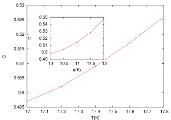
Figure 8: (Color online). The average width $D$ of the local density peaks in the ordered phase (as defined in the text), measured in units of $a_{0}$. In the main plot, results are shown versus $T$ at pin strength $s=10.K$ while in the inset $D$ is plotted versus $s$ at $T=17.0$

The width of the local density peaks of the vortex lattice at free-energy minima quantifies the degree of thermal and disorder-induced wandering of the pancake vortices from their time-averaged positions. We have studied how the average width of the local density peaks depends on $T$ and $s$. The width $D_{n,i}$ of a local density peak at computational mesh point $i$ on layer $n$ is calculated from the relation

$$D^{2}_{n,i}\equiv\frac{\sum^{\prime}_{j}r_{ij}^{2}\rho_{n,j}}{\sum^{\prime}_{j}\rho_{n,j}},$$ (7)

where $r_{ij}$ is the distance between mesh points $i$ and $j$ on the same layer, and the sum $\sum^{\prime}_{j}$ is over the mesh points on the same layer that lie inside a unit cell of the vortex lattice centered at mesh point $i$. A similar calculation was carried out in our earlier study prbv of the Lindemann parameter at the melting transition of the vortex lattice in the absence of pinning. Here, the widths of different local density peaks are not all the same, and we define the average width $D$ as the average of $D_{n,i}$ over all the local density peaks in the sample. The variation of $D$ with $T$ and $s$ is shown in Fig. 8 where we plot $D$ in units of $a_{0}$ versus $T$ at constant $s=10.0K$ in the main plot and at constant $T=17.0K$ versus $s$ in the inset. As expected, $D$ increases with $T$ for fixed $s$. The value of $D$ at a fixed $T$ increases with $s$ – the local density peaks become more distorted and broader as the pinning strength is increased. Melting of the ordered state (see next subsection) occurs when $D$ reaches a value of approximately 0.51 (this is true in all cases, not just those shown in the figure). Using the value of the equilibrium lattice constant, $a=1.988a_{0}$, for $B=0.2T$, we get the value of the Lindemann parameter, ${\mathcal{L}}\equiv D/a$, to be approximately 0.26. This is close to the value obtained for the system without pinning prbv , indicating that the Lindemann parameter at melting is nearly independent of the disorder strength $s$.

The root-mean-square (rms) lateral displacement of a pancake vortex from the average position of the vortex line to which it belongs contains another contribution, arising from the pinning-induced transverse wandering of the position of the local density peak that represents the average position of the pancake vortex. As mentioned in connection with Fig. 4, in the ordered phase the local density peaks on different layers are approximately in registry. However plots such as those in Fig. 2 indicate that there is an appreciable variation in the position of a vortex line as one moves from layer to layer – the typical width of the clusters of (blue) dots in the first panel of Fig. 2 provides a measure of this variation. We have calculated the $T$- and $s$-dependence of $D^{\prime}$, the rms displacement of the average positions of the pancake vortices that form a vortex line from the average position of the vortex line, further averaged over all vortex lines in an ordered state. The $T$-dependence of this quantity is weak in the range of temperatures considered – it increases slightly as $T$ is increased. As expected, $D^{\prime}$ increases as $s$ is increased at fixed $T$: its value in units of $a_{0}$ at $T=17.0K$ is of course zero at $s=0$, 0.16 for $s=5.0K$, 0.23 for $s=7.5K$, 0.27 for $s=10.0K$, and 0.31 for $s=12.0K$. Similar results are obtained at other temperatures. Thus, $D^{\prime}$ increases almost linearly with $s$ for relatively small values of $s$ and the rate of increase becomes smaller as $s$ is increased further. $D^{\prime}$ is typically substantially smaller than $D$ for the values of $s$ and $T$ studied. If the layer-to-layer random displacements of the average positions of the pancake vortices from the average position of the vortex line to which they belong and the lateral displacements of the pancake vortices from their average positions are assumed to be statistically independent, then the rms displacement of individual vortices from the avenge position of the vortex line would be given by $D_{net}=(D^{2}+D^{\prime 2})^{1/2}$. This would lead to values of $D_{net}$ that are $\sim$ 15% higher than those of $D$ for the largest value of $s$ ($=12.0K$) considered here. As discussed in the next subsections, these results are important for assessing the validity of the Lindemann criterion for the melting transition of the BrG state.

We end this subsection with a few comments on the structure of the disordered VL minima. As seen above, the arrangement of the vortices at these minima may be classified as amorphous, not polycrystalline. While early decoration experiments deco1 on layered high-$T_{c}$ superconductors showed evidence for an amorphous structure of the disordered phase, more recent experiments deco2 on ${\rm NbSe_{2}}$ have shown the occurrence of polycrystalline disordered structures. Also, simulations sim1 ; sim2 of the structure of two-dimensional vortex systems in the presence of random point pinning have found polycrystalline structures. Our recent work us1 ; us2 ; prbd on layered superconductors with columnar pins perpendicular to the layers also showed polycrystalline disordered states. It is therefore pertinent to inquire why polycrystalline structures are not found in the present calculation. While a complete answer to this question is not yet available, we believe that this is a consequence of the nature of the pinning potential considered here. In a sample with a small concentration of columnar pins perpendicular to the layers, the pinning potential (which is the same in all layers) is large at a few points and zero in the other parts of the sample. This favors the formation of polycrystalline structures: crystallites can form in the large “interstitial” regions where the pinning potential is zero, and since such regions on different layers are in registry, there is no conflict between the preferred arrangements of vortices on different layers. In contrast, the formation of local crystalline regions is less likely in the situation considered here because the pinning potential is nonzero at almost every computational mesh point. Also, since the pinning potentials on different layers are now completely uncorrelated, the formation of crystallites would be energetically favorable (if at all) in different regions on different layers, and such regions would, in general, not be in registry. So, the interlayer interaction that favors vortices on adjacent layers being in registry would act against the formation of crystalline patches. The last factor is, of course, absent in two-dimensional systems and less important for surface layers probed in decoration experiments. This may explain the observation of polycrystalline structures in two-dimensional simulations and some decoration experiments.

III.2 Phase diagram

We have seen then that there are two kinds of local minima of the free energy in the $(s,T)$ region we have studied. The ordered minimum is to be identified as a Bragg glass (BrG) while the disordered one is a vortex liquid (VL, whether it should be called vortex glass is discussed below).

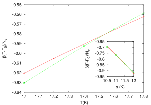
Figure 9: (Color online). Examples of the free energy per vortex, in units of $k_{B}T$, plotted versus $T$ at constant $s=10.0K$ (main plot) and versus $s$ at constant $T=17.0K$ (inset). The (red) plus signs are data for the BrG phase and the (green) crosses for the disordered phase. The data points are connected by straight lines. Statistical error resulting from pin configuration average would result in error bars smaller than the symbols. First-order transitions occur at the crossings.

Where both kinds of minima are locally stable, the equilibrium state is found by comparing their free energies, which is trivial in our procedure. The transitions then are found by looking for free energy crossings. Examples are shown in Fig. 9, where results are shown as functions of $T$ and $s$. We find that in all cases the transition is of first order: as in Fig. 9, the derivative of the free energy at the transition is discontinuous. In general, the BrG phase becomes unstable slightly above the transition: if one warms up that phase (or increases $s$) beyond the melting point one converges, after a large number of iterations, to the disordered phase. The reverse is not true, it is possible to substantially supercool the VL phase: the VL minimum remains locally stable in the whole $(s,T)$ region considered here ($0\leq s\leq 12.5K,\,16.0K\leq T\leq 21.0K$). This is consistent with experimental results andrei that suggest that the BrG phase in ${\rm NbSe_{2}}$ exhibits a spinodal instability as the temperature is increased above the transition point, whereas there is no limit of metastability of the high-temperature disordered state as it is cooled to temperatures lower than the transition temperature. This is different from the behavior found in our recent study prbd ; us1 ; us2 of the vortex system in the presence of a small concentration of random columnar pins – in that case, the high-temperature VL minimum becomes unstable as the temperature is decreased below the transition point. The absence of a spinodal instability of the VL minimum in the present case is probably related to the fact (discussed above) that the formation of large crystallites which would make the VL minimum unstable is unlikely.

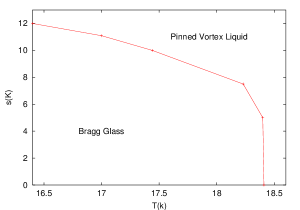
Figure 10: (Color online). Phase diagram in the $s-T$ plane at constant field $B=0.2T$. The symbols denote data points for the free energy crossings where first-order phase transitions between BrG and VL phases are found. They are connected by solid segments which thus represent the locus of first-order transitions.

From free energy results such as those shown in Fig. 9 for a variety of values of $s$ and $T$, it is possible to map the phase diagram in the $s-T$ plane. The results, averaged over all samples and at constant $B=0.2T$, are shown in Fig. 10. We can see there that, upon increasing $s$ from zero, the transition line separating the VL from the BrG is nearly vertical, and that it is only beyond $s\approx 5.0K$ that the transition line bends, while still retaining a quite appreciable $T$ dependence of the value of $s$ at which the transition occurs. The transition line trends towards being parallel to the $T$-axis at lower temperatures, indicating that the BrG phase is thermodynamically stable only if the pinning strength is lower than a “critical” value which appears to be somewhat higher than $12.0K$. Our result for the “critical” value of $s$ is in good agreement with an analytic estimate vin of this quantity for layered superconductors in the highly anisotropic limit where the electromagnetic interaction between vortices on different layers dominates over the interaction due to Josephson coupling. The general behavior of the transition temperature as a function of $s$ is in agreement with theoretical predictions gautamprl ; goldsc . The shape of the phase boundary in Fig. 10 is also very similar to that found in other numerical studies nh ; teitel2 of the BrG–VL transition. The well-known result review that the effective strength of pinning disorder in a sample with a fixed level of microscopic disorder increases with the magnetic field $B$ suggests that the phase boundary in the $B-T$ plane would have a shape similar to that in Fig. 10 with the $s$-axis replaced by the $B$-axis. This would be consistent with experimental results review . However, caution should be exercised in translating our phase diagram in the $s-T$ plane to one in the $B-T$ plane because the analogy between increasing $s$ at fixed $B$ and increasing $B$ for fixed disorder is not exact. As mentioned above, we find that the value of $D$, the average width of local density peaks at vortex positions as defined below Eq. (7), remains nearly constant along the phase boundary. This supports approximate analytic calculations goldsc ; nelson based on the assumption that the melting transition of the BrG phase occurs at a constant value of the Lindemann parameter ${\mathcal{L}}$. However, our results also show that if the quantity $D_{net}$, which measures the rms displacement of vortices from the average position of the vortex line to which they belong (see discussion in the paragraph following that including Eqn. (7)), is used to define ${\mathcal{L}}$, then it would not remain constant along the phase boundary – it would increase by about 15% as the disorder strength is increased from zero to $12.0K$. Since the vortex positions on different layers are close to registry in the BrG phase, while the interlayer correlations in the vortex positions are very weak in the VL phase (see Figs. 2 and 4), the BrG–VL transition may be thought of as a “decoupling” transition glaz at which the correlation between vortex positions on different layers drops abruptly.

We do not find evidence for a VG phase thermodynamically distinct from the high-temperature VL in the range of pin strengths and concentrations studied. The VL minimum obtained at relatively high temperatures evolves continuously as $T$ decreases. The degree of localization of the vortices, measured by the typical heights of the local density peaks at the free-energy minimum, does increase as $T$ is reduced, but the change is smooth. We found no evidence of a phase transition between a weakly pinned and a strongly pinned distinct VL states. This leads us to classify all disordered minima at low temperatures and relatively large pinning strengths as strongly pinned VL, to distinguish them from the more liquid-like disordered minima obtained for higher $T$ and smaller $s$. We have carried out various thermal “cycling” procedures (such as warming up the disordered minimum obtained by quenching a liquid-like initial configuration to a low temperature, and cooling the VL minimum obtained at a high temperature) for various values of $s$ to look for local minima that are different from the BrG and VL ones. We did not find (see also below) any other minimum that could be classified as a VG that is structurally and thermodynamically different from the VL. Thus, we conclude that our system does not exhibit a distinct equilibrium VG phase in the region studied. Since the interaction between straight vortex lines is screened in the model considered here, such a conclusion would be consistent with the expectation bokil that a VG phase does nor exist in three dimensions if electromagnetic screening of inter-vortex interactions is taken into account. However, such a drastically general inference would be unwarranted. Also, our mean-field calculation that considers only the density variables can not rule out the occurrence of a continuous VL-VG transition with subtle characteristics (such as the continuous transition suggested by the experimental results of Ref. zeldov, , for which structural signatures and the nature of the order parameter are particularly hard to identify), or one in which the phase of the superconducting order parameter (not included in our treatment) plays a crucial role.

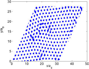
Figure 11: (Color online). Intermediate non-equilibrated multi-domain state obtained at $s=9.0K$, $T=17.0K$ as explained in the text. As in Fig. 2, the average position of each vortex is represented by a dot.

We mentioned in Section I that earlier studies have suggested the occurrence of other phases for the system considered here. These include a “vortex slush” phase nh predicted to exist at intermediate values of $T$ just above the boundary of the the BrG phase in the $s-T$ plane, and a “domain glass” phase gautam expected between the BrG and VL phases for relatively small values of $s$. It has been shown teitel that the vortex slush “phase” found in the simulation of Ref. nh, corresponds to vortex configurations nearly crystalline in each layer, but with the vortices on different layers not being in registry: the orientation of the reciprocal lattice vectors that describe the crystalline order on different layers varies from layer to layer. The domain glass phasegautam is supposed to consist of large crystalline domains. We have looked for the existence of free-energy minima that may represent such phases. In our attempts, we artificially made the VL minimum unstable towards the formation of crystalline structures by multiplying the $C_{mn}(r)$ used as input in our calculations by a factor of 1.05, which makes the structure factor $\tilde{S}({\bf k},k_{z})\equiv 1/[1-\rho_{0}C({\bf k},k_{z})]$ negative for $k_{z}=0$ and $k$ close to the magnitude of the smallest reciprocal lattice vectors of the triangular vortex lattice. Our expectation was that the system would then converge to one of the other kinds of minima mentioned above, if they existed. In these calculations, we started with liquid-like initial conditions and quenched to within the region (low $T$, moderately large values of $s$) where these phases are expected. The minimization routine was run for a large number of iterations with the modified $C_{mn}(r)$, so that the instability of the VL minimum resulted, indeed, in the formation of locally crystalline structures on the layers. Configurations obtained at different stages of this run were then used as inputs in minimization runs in which we slowly eliminated the modification in $C_{mn}(r)$ so as to recover the original, physical interaction. In all such runs, the system converged to the BrG state but very slowly: the number of iterations it took for convergence was over twenty times larger than that in the ordinary case. The system lingered for a very large number of iterations in a multi-domain state. The ultimate convergence was always to minima with the vortices on different layers in registry, even when the vortices were very much out of registry in the intermediate configuration. An example is shown in Fig. 11, at $s=9.0K$, $T=17.0K$ where the vortex positions for an intermediate state with multi-domain structure are shown in a plot similar to those in Fig. 2. The converged state, however, turned out to be a single domain BrG very similar to that shown in the first two panels of Fig. 2.

These results argue against the existence of the other phases suggested in earlier studies, at least in the region of pinning strength and concentration studied, as thermodynamic equilibrium phases. However, that the system remains in a polycrystalline state for a large number of iterations in the minimization process suggests that such states may be stabilized through changes in the model parameters or may correspond to long-lived transient situations. Further investigations of this possibility would be interesting. On the other hand, the reported observation of this phase in simulations might result from using a small system size or insufficient equilibration, or both. In our samples, the number of layers and the number of vortices on each layer are substantially larger than those in the simulations of Ref. nh, . Also, the interlayer interaction in our model is rather weak, since we consider only the electromagnetic interaction between vortices on different layers. The system nevertheless converges to a BrG minimum with vortices on different layers in registry, which implies that a vortex slush in which vortices form crystalline arrangements on the layers, but the arrangements on different layers are not in registry is rather unlikely to occur as a thermodynamic phase.

III.3 Distribution of local magnetic induction

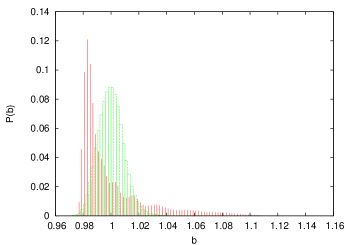
Figure 12: (Color online) The probability distribution for fields $P(b)$ in terms of the dimensionless field $b$ at $T=18.4K$ and $s=5.0K$, which is very near the melting point. The (red) solid lines are for the BrG state and the (green) blocks are for the VL state.

Finally, we give a brief discussion of our results for the distribution of the local, microscopic, magnetic induction in the superconductor. This is a quantity of considerable experimental interest, as it can be measured directly in $\mu$SR experimentsmusrrev . The probability distribution of the local magnetic induction is easily computedmusr from the vortex density distribution at the minima. We consider the the component of the magnetic induction perpendicular to the layers. The Fourier transform of this $z$-component due to a single pancake vortex at the origin is given by musr

$$b_{z}({\bf k},k_{z})=\frac{d\Phi_{0}}{1+\lambda^{2}k^{2}+\lambda^{2}k_{z}^{2}},$$ (8)

where $d$ is the spacing between the layers and $\lambda$ the penetration depth in the layer plane. If the typical time scales for the dynamics of density fluctuations in the state the vortex system is in are much shorter than the characteristic time scale of muon spin precession, the muons see a broadened (time-averaged) density distribution of the vortices. The time-averaged local magnetic field $B_{z}$ is then obtained through a convolution of the local density at a free-energy minimum with the expression for $b_{z}$ given in Eq.(8). If the dynamic time scales for such fluctuations are much longer than the precession time of the muon spins, then the convolution is to be done musr using a local density consisting of two-dimensional $\delta$-functions located at the local density peaks at the free-energy minimum. The time scales are beyond the scope of our time averaged calculation, but both methods give very similar results in any case.

We have used these procedures to calculate the distribution of $B_{z}$ for different free-energy minima. In our discretized system, the convolution is done using discrete Fourier transforms, leading to the values of $B_{z}$ at the computational mesh points. These values are binned to yield histograms for the distribution of $B_{z}$. The results are best represented in terms of the dimensionless field $b\equiv B_{z}/B$. An example is given in Fig. 12 at a point on the melting curve. The two states clearly have different probability distributions $P(b)$, with that corresponding to the VL state being narrower and much more symmetric. The distribution for the BrG state shows a long “tail” in the large-$b$ side. All these features are very similar to experimental results musrrev ; lee1 . The results shown in Fig. 12 were obtained using the locations of the vortices at the minima – the distributions obtained from the time-averaged local density have the same shape, but are somewhat narrower in the VL phase.

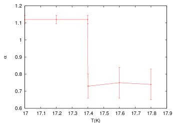
Figure 13: (Color online). The parameter $\alpha$ characterizing the degree of asymmetry of the probability distribution $P(b)$ (see Figure 12) plotted as a function of $T$ at $s=10.0K$. The result plotted at each temperature is the value for the equilibrium state at that temperature, averaged over pin configurations.

The degree of asymmetry of $P(b)$ can be conveniently characterizedmusrrev by introducing a dimensionless parameter $\alpha$ defined as the ratio of the cube root of the third moment of $P(b)$ to the square root of its second moment. This parameter changes discontinuously at melting. An example is shown in Fig. 13 where $\alpha$ is plotted as a function of $T$ at constant $s=10.0K$. Results are given for the equilibrium state at each temperature and averaged over four pin configurations. It turns out that for the VL state (but not for the BrG), the results for $\alpha$ vary appreciably from one pin configuration to another (the only quantity we have found that does so) and also depending on which of the two methods (local density peaks or full density) is used. We have therefore averaged also over the two methods. The resulting error bars are still larger in the VL state as the distribution in that case is close to being symmetric and rather small changes in the shape of $P(b)$ lead, in that situation, to considerable changes in $\alpha$. The results for $\alpha$ are quantitatively similar to those of $\mu$SR experiments lee1 on the BrG-VL transition in BSCCO induced by increasing the magnetic field at a fixed temperature. A similar discontinuity in the value of $\alpha$ is also observed lee2 at the melting of the BrG phase upon increasing the temperature at fixed $B$. However, the value of $\alpha$ in the VL phase is found lee2 to be negative in that case. The reason for the negative value of $\alpha$ is not completely clear. It has been attributed to effects of sample geometry musrrev and it has been argued divakar that a negative $\alpha$ indicates the presence of a multi-domain state. Since effects of sample geometry are not present in our calculations with periodic boundary conditions and we do not find any multi-domain state, it is perhaps not surprising that our calculations do not yield negative values of $\alpha$.

IV Conclusions

We have studied in this paper the phase diagram of the superconducting vortex lattice in a layered superconductor, in the presence of both a magnetic field normal to the layers and of random atomic-scale point pinning centers. We have considered the strongly anisotropic case where the interactions are of two-body form and the free energy can then be written as a functional of the time averaged vortex density. Numerical minimization of the discretized free energy then yields the pancake vortex density distribution at the minima.

The values of the free energy at the minima can be plotted to locate the phase transitions. Our main result is the phase diagram (Fig. 10) in the temperature – pin strength plane, where we find a line of first-order phase transitions between a Bragg glass and a disordered phase. The density distributions at the minima can then be analyzed to obtain any desired correlation functions. They can also be used to directly visualize the vortex lattice in real space and to obtain the distribution of the microscopic local magnetic induction in the superconductor. From an extensive analysis of such results we conclude that the disordered phase is to be identified as a pinned vortex liquid. While one can distinguish between strong and weak pinning regimes, the crossover between them is completely smooth.

As discussed in detail in the previous section, our results are consistent with those of experiments and simulations, the only possible exception being that we do not find, in the region of pinning strength and concentration studied, any sign of additional “vortex glass”, “vortex slush” or “domain glass” phases the existence of which has been made at least plausible by results obtained e.g. in Refs. zeldov, ; nh, ; gautam, respectively. We have ourselves found prbd ; us1 ; us2 a polycrystalline Bose glass phase in the case of columnar pinning through the use of the same methods as in this work. Such phases may exist under other conditions, specifically for a much smaller concentration of considerably stronger defects which would favor polycrystallinity much more than the situation studied here, where we have chosen a value of the concentration $c$ of atomic defects which, although small in the atomic scale, is in a sense large with respect to the vortex lattice: there are many pinning sites per vortex lattice unit cell. The results for columnar pinning, where the concentration is much smaller but the pinning strength larger, make it possible to conjecture that there is a regime of larger $s$ but smaller $c$ where additional phases may exist. Further work in that direction is clearly worthwhile.

In a paper rodri that appeared after this one was originally submitted, it has been suggested, from an analysis of a disordered $xy$ model in which electromagnetic interactions between vortices is neglected, that the BrG phase should become unstable (no matter how weak the pinning) to disorder in the direction normal to the layers at a value of $B$ smaller than that considered here. Our results for the correlation function $g(0,n)$ as a function of interlayer separation $n$ in the ordered phase (discussed in the text in connection with Fig. 4), indicate no decay in this quantity as a function of $n$ in the region $3<n\lesssim N_{L}/2$. Further, as mentioned above, our phase diagram data quantitatively agree with analytic calculations vin in which the softening of the tilt modulus at large wavelengths was included. These results strongly argue for the actual stability of the BrG phase, in agreement with previous numerical studies nh ; teitel2 of the disordered $xy$ model. However, even though our samples are already, as noted, much thicker than those considered in earlier numerical studies nh ; teitel2 , the possibility that the BrG phase would disorder in the transverse direction over a length scale much larger than $\lambda$ can not be mathematically ruled out by our numerical results.

- (1) G. Blatter, M.V. Feigelman, V. B. Geshkenbein, A. I. Larkin, and V. M. Vinokur, Rev. Mod. Phys. 66, 1125 (1994).
- (2) T. Nattermann, Phys. Rev. Lett. 64, 2454 (1990).
- (3) T. Giamarchi and P. Le Doussal, Phys. Rev. B 52, 1242 (1995).
- (4) T. Klein, I. Joumard, S. Blanchard, J. Marcus, R. Cubitt, T. Giamarchi and P. Le Doussal, Nature (London) 413, 404 (2001).
- (5) M. P. A. Fisher, Phys. Rev. Lett. 62, 1415 (1989).
- (6) D. S. Fisher, M.P.A. Fisher and D.A. Huse, Phys. Rev. B 43, 130 (1992).
- (7) R. H. Koch, V. Foglietti, W. J. Gallagher, G. Koren, A. Gupta, and M. P. A. Fisher, Phys. Rev. Lett. 63, 1511 (1989). For more recent work along similar lines, see A. M. Petrean, L. M. Paulius, W.-K. Kwok, J. A. Fendrich, and G. W. Crabtree, Phys. Rev. Lett. 84, 5852 (2000) and references therein.
- (8) D. R. Strachan, M. C. Sullivan, P. Fournier, S. P. Pai, T. Venkatesan, and C. J. Lobb, Phys. Rev. Lett. 87, 067007 (2001).
- (9) H. Beidenkopf, N. Avraham, Y. Myasoedov, H. Shtrikman, E. Zeldov, B. Rosenstein, E. H. Brandt, and T. Tamegai, Phys. Rev. Lett. 95, 257004 (2005).
- (10) H. S. Bokil and A. P. Young, Phys. Rev. Lett. 74, 3021 (1995); J. Kisker and H. Rieger, Phys. Rev. B 58, R8873 (1998).
- (11) P. Olsson, Phys. Rev. B 72, 144525 (2005)
- (12) J. Lidmar, Phys. Rev. Lett. 91, 097001 (2003); A. Vestergren, J. Lidmar, and M. Wallin, Phys. Rev. Lett. 88, 117004 (2002).
- (13) Y. Nonomura and X. Hu, Phys. Rev. Lett. 86, 5140 (2001).
- (14) P. Olsson and S. Teitel, Phys. Rev. Lett. 94, 219703 (2005). See also Y. Nonomura and X. Hu, Phys. Rev. Lett 94, 219704 (2005).
- (15) S. S. Banerjee, A. K. Grover, M. J. Higgins, G. I. Menon, P. K. Mishra, D. Pal, S. Ramakrishnan, T.V. Chandrasekhar Rao, G. Ravikumar, V. C. Sahni, S. Sarkar, and C. N. Tomy, Physica C 355, 39 (2001), and references therein.
- (16) G. I. Menon, Phys. Rev. B 65, 104527 (2002).
- (17) C. Dasgupta and O.T. Valls, Phys. Rev. B66, 064518 (2002).
- (18) C. Dasgupta and O.T. Valls, Phys. Rev. B72, 094501 (2005).
- (19) T. V. Ramakrishnan T.V. and M. Yussouff, Phys. Rev. B 19 (1979).
- (20) P. Olsson and S. Teitel, Phys. Rev. Lett. 87, 137001 (2001).
- (21) Z. L. Xiao, O. Dogru, E.Y. Andrei, P. Shuk, and M. Greenblatt, Phys. Rev. Lett. 92, 227004 (2004).
- (22) J. E. Sonier, J. H. Brewer and R. F. Kiefl, Rev. Mod. Phys. 72, 769 (2000).
- (23) A.V. Rozhkov, Phys. Rev. B 73, 134520 (2006).
- (24) J. P. Hansen and I.R. McDonald, Theory of simple liquids, (Academic Press, London, 1986).
- (25) G. I. Menon, C. Dasgupta, H. R. Krishnamurthy, T. V. Ramakrishnan and S. Sengupta, Phys. Rev. B 54, 16192 (1996).
- (26) C. Dasgupta, Europhysics Lett, 20, 131 (1992).
- (27) G. I. Menon and C. Dasgupta, Phys. Rev. Lett. 73, 1023 (1994).
- (28) D. J. Grier, C. A. Murray, C. A. Bolle, P. L. Gammel, D. J. Bishop, D. B. Mitzi and A. Kapitulnik, Phys. Rev. Lett. 66, 2270 (1991).
- (29) Y. Fasano, M. Menghini, F. de la Cruz, Y. Paltiel, Y. Myasoedov, E. Zeldov, M. J. Higgins, and S. Bhattacharya, Phys. Rev. B 66, 020512(R) (2002).
- (30) M. Chandran, R. T. Scalettar, and G. T. Zimanyi, Phys. Rev. B 69, 024526 (2004).
- (31) S.S. Ghosh and C. Dasgupta, manuscript in preparation.
- (32) C. Dasgupta and O. T. Valls, Phys. Rev. Lett. 91, 127002 (2003).
- (33) C. Dasgupta and O. T. Valls, Phys. Rev. B 69, 214520 (2004).
- (34) A.E. Koshelev and V.M. Vinokur, Phys. Rev. B57, 8026 (1998).
- (35) Y. Y. Goldschmidt, Phys. Rev. B 56, 2800 (1997).
- (36) D. Ertaz and D.R. Nelson, Physica C 272, 79 (1996).
- (37) L. I. Glazman and A.E. Koshelev, Phys. Rev B 43, 2835 (1991).
- (38) G. I. Menon, C. Dasgupta and T. V. Ramakrishnan, Phys. Rev. B 60, 7607 (1999).
- (39) S. L. Lee, P. Zimmermann, H. Keller, M. Warden, I.M. Savic , R. Schauwecker, D. Zech, R. Cubitt, E.M. Forgan, P.H. Kes, T. W. Li, A.A. Menovsky, and Z. Tarnawski, Phys. Rev. Lett. 71, 3862 (1993).
- (40) S. L. Lee, C. M. Aegerter, H. Keller, M. Willemin, B. Stauble-Pumpin, E. M. Forgan, S. H. Lloyd, G. Blatter, R. Cubitt, T. W. Li and P. Kes, Phys. Rev. B 55, 5666 (1977).
- (41) U. Divakar, A. J. Drew, S. L. Lee, R. Gilardi, J. Mesot, F.Y. Ogrin, D. Charalambous, E.M. Forgan, G. I. Menon, N. Momono, M. Oda, C. D. Dewhurst, and C. Baines, Phys. Rev. Lett. 92, 237004 (2004).
- (42) J.P. Rodriguez, Phys. Rev. B73, 214520 (2006).