Topological Entanglement Entropy from the Holographic Partition Function

Abstract

We study the entropy of chiral 2+1-dimensional topological phases, where there are both gapped bulk excitations and gapless edge modes. We show how the entanglement entropy of both types of excitations can be encoded in a single partition function. This partition function is holographic because it can be expressed entirely in terms of the conformal field theory describing the edge modes. We give a general expression for the holographic partition function, and discuss several examples in depth, including abelian and non-abelian fractional quantum Hall states, and $p+ip$ superconductors. We extend these results to include a point contact allowing tunneling between two points on the edge, which causes thermodynamic entropy associated with the point contact to be lost with decreasing temperature. Such a perturbation effectively breaks the system in two, and we can identify the thermodynamic entropy loss with the loss of the edge entanglement entropy. From these results, we obtain a simple interpretation of the non-integer ‘ground state degeneracy’ which is obtained in 1$+$1-dimensional quantum impurity problems: its logarithm is a 2$+$1-dimensional topological entanglement entropy.

I Introduction

Entanglement is one of the characteristic peculiar features of quantum mechanics. It lay at the heart of the debates between Bohr and Einstein, Podolski, and Rosen, and it is essential for the Bell’s inequality violation which distinguishes quantum mechanics from classical hidden variables theories. Entanglement between logical qubits is a resource for quantum computation; entanglement between physical qubits and the environment is a threat to quantum computation; entanglement between physical qubits is essential for error correction.

Entanglement entropy is one measure of entanglement. If a system can be subdivided into two subsystems $A$ and $B$, then even if the whole system is in a pure quantum state $|\Psi\rangle$, subsystem $A$ will be in a mixed state with density matrix $\rho$ obtained by tracing out the subsystem $B$ degrees of freedom:

$$\rho_{A}=\text{tr}_{B}\bigl{(}\left|\Psi\right\rangle\!\left\langle\Psi\right|\bigr{)}$$ (1)

The entropy of this density matrix will be zero if the state $|\Psi\rangle$ is the direct product of a pure state for subsystem $A$ with a pure state for subsystem $B$ or, equivalently, if the matrix ${\rho_{A}}$ has only a single non-zero eigenvalue. If the entropy

$${{\cal S}_{A}}=-\text{tr}\!\left({\rho_{A}}\ln{\rho_{A}}\right)$$ (2)

is non-zero, then the subsystems $A$ and $B$ are entangled.

The entanglement entropy ${\cal S}_{A}$ is a measure of the correlations between the degrees of freedom of the $A$ and $B$ subsystems. In a $1$+$1$-dimensional quantum system, the dependence of ${\cal S}_{A}$ on the length $L$ of subsystem $A$ can be used to distinguish critical from non-critical systems: it remains finite as the length increases, except at criticality, where it diverges logarithmically with a universal coefficient Holzhey94 ; Calabrese04 . Of course, in this case, there are other measures of criticality, such as the power-law decay of correlation functions. In a gapped system, the leading term in the entanglement entropy is proportional to the surface area of the boundary. The coefficient is cutoff-dependent. However, in a $2+1$-dimensional system in a gapped topological phase, the first subleading term is universal and independent of the size or shape of $A$ Kitaev05 ; Levin05 :

$${{\cal S}_{A}}=aL-\ln{\cal D}+\ldots$$ (3)

It is not immediately obvious that ${\cal D}$ in the above equation (3) is uniquely defined since $a$ is a cutoff-dependent coefficient (in two spacetime dimensions, the ‘surface area’ is the length of the boundary). However, by dividing a system into three or more subsystems and forming an appropriate linear combination of the resulting entanglement entropies, the length term can be canceled, leaving only the universal term Kitaev05 ; Levin05 . Such a construction can be used to give a more precise definition of the topological entanglement entropy, but its essential meaning is captured by (3). The quantity ${\cal D}$ is the total quantum dimension of the topological phase, which we define in section II.

This is potentially a very useful probe of a topological phase. In such a phase, all correlation functions are topologically-invariant at distances longer than some finite correlation length and energies lower than a corresponding energy scale. Hence, in order to identify such a state, one must examine the ground state degeneracy on higher-genus surfaces or the braiding properties of quasiparticle excitations. The entanglement entropy gives us a handle on this topological structure stemming from the ground state wavefunction alone.

Topological quantum field theories (TQFTs) were widely studied in the string-theory community in the late ’80s and early ’90s, following Witten’s celebrated work Witten89 on Chern-Simons field theory, conformal field theory (CFT), and the Jones polynomial of knot theory Jones85 . There has been a recent revival of interest in TQFTs due to the possible emergence of topological phases in electronic condensed-matter systems and the proposed use of such phases as a platform for fault-tolerant quantum computation Kitaev97 ; Physics-Today . The above definition of a topological phase can be compactly (though tautologically) restated as a phase of matter for which the long-distance effective field theory is a topological field theory. The entanglement entropy is a way of extracting one of the basic parameters of a topological field theory, its quantum dimension.

A chiral TQFT in $2$+$1$ dimensions is related to $1$+$1$-dimensional rational conformal field theory (RCFT) in several ways. When the TQFT is defined on a manifold with boundary, the boundary degrees of freedom form an RCFT. The topological invariance of the theory means that there is no distinction between spacelike and timelike boundaries. Hence, the RCFT describes both (a) the ground state wavefunction(s) at some $(2$+$0)$-d equal-time slice when spacetime is $M\times I$, for a compact surface $M$ and time interval $I$, and (b) the dynamics of the $(1$+$1)$-d boundary when spacetime is $X\times R$, where $X$ is a surface with boundary. In the RCFT, the topological braiding/fusion structure of the TQFT is promoted to a holomorphic structure with branch cuts implementing non-trivial monodromies. This structure occurs in the TQFT ground state(s) (the $(2$+$0)$-d case) as a result of the choice of holomorphic gauge. In the $(1$+$1)$-d case, however, it represents the actual critical dynamics of the excitations of the edge of the system.

Although other possible settings are also suspected, there is only one place in nature where topological phases are known for certain to exist: the quantum Hall regime. In this regime, this ‘holographic’ relationship between the $(2$+$1)$-d TQFT describing the bulk and the $(1$+$1)$-d RCFT describing edge excitations is beautifully realized. Since it is easier to experimentally probe the edge, the topological properties of quantum Hall states have, thus far, been mostly probed through the constraints that they place on the dynamics of the edge.

One can continue to still lower dimensions and consider boundaries or defect lines in $2d$ classical critical systems and impurities in $(1$+$1)$-d quantum critical systems with dynamical critical exponent $z=1$. (In many $(2$+$1)$-d or $(3$+$1)$-d critical systems, only the $s$-wave channel interacts with the impurity. By performing a partial wave decomposition and keeping only this channel, one can map the problem to a $(1$+$1)$-d problem. Hence, the restriction to $(1$+$1)$-d is not very severe.) In these situations, the constraints of conformal invariance in the bulk strongly constrain the low-energy behavior of the boundary/defect correlations or impurity dynamics. The same methods can be applied to a point contact in a $(2$+$1)$-d system in a topological phase. The point contact allows tunneling between the gapless excitations at the edge and can, therefore, be understood as an impurity in a $(1$+$1)$-d system.

In particular, we can write the entropy of the impurity problem as

$${\cal S}_{\hbox{imp}}=fL+\ln(g)\ +\ \dots$$ (4)

where $L$ is the size of one-dimensional space. The leading piece is non-universal, but a universal part of the entanglement entropy proportional to the central charge of the conformal field theory can be extracted Casini04 . In this paper, we will focus on subleading pieces of the entropy like $\ln(g)$. Although $\ln(g)$ is often called the “boundary entropy”, we see that this interpretation is not always useful: we will see how such a term can be present even when there is no boundary to the $1$+$1$ dimensional system. Moreover, if it were truly the entropy of the impurity, then $g$ would be an integer. However, if one computes it by first taking the thermodynamic limit $LT\to\infty$, and then taking $T\to 0$, $g$ is not always an integer Andrei84 ; Tsvelik85 ; Cardy89 ; Affleck91 . This makes this subleading contribution to the entropy somewhat mysterious to interpret physically.

To make this clearer, we will examine in detail the situation in which the $(1$+$1)$-d critical system is the edge of a $(2$+$1)$-d system in a chiral topological phase. In particular, we will show that the value of $g$ in (4) is closely related to that of the quantum dimension ${\cal D}$ of the topological quantum phase, that occurs in the entanglement entropy in (3). Although they are both subleading terms in entropies, their relation is far from obvious. Indeed, their very definitions are quite different, involving an interchanged order of limits. The entanglement entropy is a property of the ground state obtained in the zero temperature limit, when the region size $L$ is subsequently taken to infinity. On the other hand, extracting the subleading $\ln(g)$ correction of the thermodynamic entropy as in (4) requires taking $L$ to infinity before taking the zero temperature limit. Despite this opposite ordering of limits, we will show that both quantities follow from the same deep results in conformal field theory Cardy89 ; Verlinde88 ; Moore88 .

The connection can be understood heuristically by considering the entropy loss resulting from the impurity/point contact as the temperature is decreased. This is convenient because it allows one to get rid of the contributions proportional to $L$ by considering the difference ${\cal S}_{UV}-{\cal S}_{IR}$, where ${\cal S}_{UV}$ is the entropy in the absence of the impurity/point contact (the ultraviolet limit), and ${\cal S}_{IR}$ is the entropy in the zero-temperature limit (the infrared limit). In the IR limit, the point contact in the topological theory effectively cuts the edge in two. When the edge is cut into two, the topological entanglement entropy (3) receives a contribution $-2\ln{\cal D}$. Thus ${\cal S}_{UV}-{\cal S}_{IR}=\ln{\cal D}$. As we will see, by definition, ${\cal D}>1$, so this is indeed positive as one expects for a flow caused by a relevant perturbation. This demonstrates that a “$g$-theorem” Affleck91 ; Friedan04 applies to a point contact across a system in a topological phase. Likewise, in quantum impurity problems the impurity degrees of freedom end up being screened (at least partially) by coupling to the degrees of freedom in the one-dimensional bulk.

These results show that when a $(1$+$1)$-d critical system is the boundary of a $(2$+$1)$-d system in a topological phase, the thermodynamic “boundary entropy” of eq. 4 is actually the topological entanglement entropy for the subsystems into which the system has been dynamically split. This is reminiscent of the generation of entropy by black hole formation. (The reader need not worry that by relating a $(0$+$1)$-d entropy to a $(2$+$1)$-d entropy we are forgetting that a boundary cannot have a boundary. The point contact is not the boundary of a $(1$+$1)$-d system, but rather a defect in the middle of it – and, therefore, capable of cutting it in two.)

In fact, the connection between the two kinds of entropy goes even deeper. When a topological phase has quasiparticles with non-Abelian statistics, there is an additional source of entanglement entropy. This arises because the Hilbert space for identical particles obeying non-Abelian statistics must be multi-dimensional (even when ignoring the position and momentum of the particles), so that the system moves around in this space as the quasiparticles are braided. For example, in a $p+ip$ superconductor, two vortices form a two-state quantum system, which therefore have an entanglement entropy $\ln(2)$. We dub this entropy the bulk entanglement entropy, because it comes from the gapped bulk quasiparticles. However, we emphasize that this a subleading piece of the 2$+$1-dimensional bulk entropy: it is independent of the size of the system, but rather depends only on the number and type of quasiparticle excitations in a given state. The remarkable connection is that this part of 2$+$1 dimensional bulk entropy can be encoded in a 1$+$1 dimensional partition function. In other words, the entanglement entropy of these bulk quasiparticles is a property of the boundary of the system (just like a black hole!). We show how to compute such holographic partition functions by using conformal field theory.

In section II, we discuss the quantum dimensions of a topological state and of the various quasiparticle excitations of such a state. We give a general way to compute quantum dimensions using conformal field theory in section III, and do this computation for a variety of examples in appendix A. The examples include the Laughlin states for the abelian fractional quantum Hall effect, the Moore-ReadMoore91 and Read-RezayiRead99 non-abelian quantum Hall states, and the $p+ip$ superconductorGreiter92 ; Read00 . In section IV we derive the central results of our paper, which define the holographic partition function and how it describes the topological entanglement entropy. We show in section V how these results can be applied to understand how a point contact affects the entropy. This complements recent results of ours, relating point contacts in the Moore-Read state and in $p+ip$ superconductors to the Kondo problem Fendley06a ; Fendley06b .

II Quantum dimensions

A fundamental characteristic of a topological field theory is the quantum dimensions of the excitations. The topological entanglement entropy of the systems studied here on a space with smooth boundaries is entirely given in terms of these numbers.

For the quantum Hall effect and related states, one can find the quantum dimensions directly from the wavefunctions Nayak96c ; Read96 . In this paper we find it useful to instead compute them using the methods of conformal field theory. The formal reason why this is possible is that the algebraic structure of rational conformal field theory is virtually identical to that of topological field theory (this can be understood precisely by using the mathematical language of category theory). A more intuitive reason is that the gapless edge modes of the 2$+$1-dimensional quantum theories studied here form an effectively 1$+$1 dimensional system. A 1$+$1-dimensional gapless system with linear dispersion has conformal invariance, so the powerful methods of conformal field theory are applicable. The edge modes are in one-to-one correspondence with the modes of the bulk system, so the $d_{a}$ computed using conformal field theory are those of the bulk system as well.

We introduce the full conformal field theory formalism in the next section. In this section we explain how to define both the individual quantum dimensions of the quasiparticles $d_{a}$, and the total quantum dimension ${\cal D}$ of a theory. We discuss explicitly the simplest non-trivial example, the Ising model.

The quantum dimension is simple to define. Denote the number of linearly-independent states having ${\cal N}$ quasiparticles of type $a$ as $H_{a}({\cal N})$. Then the quantum dimension $d_{a}$ of the excitation of type $a$ is given by studying the behavior of $H_{a}({\cal N})$ for large ${\cal N}$, which behaves as

$$H_{a}({\cal N})\propto d_{a}^{\cal N}\ .$$

To have non-abelian statistics, one must have $d_{a}>1$; these degenerate states are the ones which mix with each other under braiding. In such a situation one typically has $d_{a}$ which are not integers.

As we discussed in the introduction, the topological entanglement entropy is related to the total quantum dimension ${\cal D}$, which is defined as

$${\cal D}=\sqrt{\sum_{a}d_{a}^{2}}.$$ (5)

The sum is over all the types of quasiparticles in the theory. Thus to compute ${\cal D}$, one must not only compute the $d_{a}$ but be able to classify all the different quasiparticles as well. Since $d_{a}\geq 1$ by definition, for ${\cal D}$ to make sense there can only be a finite number of different quasiparticles. We must therefore confine ourselves to topological field theories where this is true. Luckily, the topological theories of most importance in condensed-matter physics have this property.

We will give a simple expression for ${\cal D}$ below in terms of the modular $S$ matrix of conformal field theory, but here we illustrate how it comes about. In the fractional quantum Hall effect there is a very natural way of understanding the structure of the topological theory. Quasiparticle states are defined “modulo an electron”. This means that in the topological theory, two excitations which differ by adding or removing an electron are treated as equivalent. Thus the charge-$e$ electron is in the identity sector of the theory, since in the topological theory the identity and the electron are equivalent.

A simple example is in the abelian Laughlin states at filling fraction $\nu=1/m$. We discuss in depth in the appendix how the consequence of modding out by an electron is that states differing in charge by any integer times $e$ are identified in the topological theory. Only fractionally-charged quasiparticles result in sectors other than the identity. In the Laughlin states, the fundamental quasiparticle has charge $-1/m$. One can obviously consider more than one of these to get larger fractional charge, but if one has $m$ of the fundamental quasiparticles, they can fuse into a hole (put another way, the hole can split apart into $m$ fundamental quasiparticles). Different sectors of the topological theory can therefore be labeled by the charges $ae/m$ where $a$ is an integer obeying $0\leq a<m$. There are thus $m$ different quasiparticle sectors. The quantum dimension of any quasiparticle in an abelian theory is $1$, so we have $d_{a}=1$ for $a=0\dots m-1$. Using this with (5) gives the total quantum dimension of a Laughlin state at $\nu=1/m$ to be

$${\cal D}_{\nu=1/m}=\sqrt{m}.$$ (6)

Finding ${\cal D}$ for non-abelian states requires knowing even more about the structure of the theory. Not only does it require knowing what the quasiparticles are, but finding the individual $d_{a}$ requires knowing what the fusion rules are. The fusion rules describe how to treat multi-particle states in the topological phase in terms of single-particle states. In the abelian case, the fusion rules are simple: for example, two charge-$e/m$ particles fuse to effectively give a single charge-$2e/m$ particle. The non-abelian structure of the theory arises when two particles can fuse in more than one way.

We illustrate this in the $p+ip$ superconductor. As discussed in detail in a number of places Read00 ; Ivanov01 , a vortex has a Majorana fermion zero mode in its core. Then two vortices share a Dirac fermion (=2 Majorana fermions) zero mode. This zero mode can be either empty or filled; thereby, two vortices form a two-state system. Denoting the identity sector by $I$, the vortex by $\sigma$ and the filled zero mode by $\psi$, this means that the fusion rule for two vortices can be denoted by $\sigma\cdot\sigma=I+\psi.$ Two different terms on the right-hand-side means that there are two ways to fuse two sigma quasiparticles. (More precisely, this means that two vortices have a two-dimensional Hilbert space.) One finds that the full set of fusion rules here are

$$\psi\cdot\psi = I$$

$$\sigma\cdot\sigma = I\ +\ \psi$$ (7)

$$\psi\cdot\sigma = \sigma$$

and, of course, fusion with the identity gives the same field back.

The quantum dimensions follow from the fusion rules. Two $\sigma$ quasiparticles here can fuse to give either the identity $I$, or the fermion $\psi$. Thus while $H_{\sigma}(1)=1$, these two possibilities for fusion of $\sigma$ with itself means that the dimension of the Hilbert space for two vortices is $H_{\sigma}(2)=2$. Now include a third vortex. The dimension of the Hilbert space is not $4$, but rather is $H_{\sigma}(3)=2$. This is because

$$\sigma\cdot\sigma\cdot\sigma=(I+\psi)\cdot\sigma=\sigma+\sigma.$$

Fusion is associative, so it makes no difference in which order we fuse. Continuing in this fashion, it is easy to see that

$$H_{\sigma}(\cal N)=\begin{cases}2^{{\cal N}/2}\qquad\qquad&{\cal N}\hbox{ even}\\ 2^{({\cal N}-1)/2}\qquad\quad&{\cal N}\hbox{ odd}\\ \end{cases}$$

The quantum dimension of the vortex is therefore $d_{\sigma}=\sqrt{2}$. Since $\psi\cdot\psi=I$, $H_{\psi}({\cal N})=1$ for all ${\cal N}$, so the quantum dimension of the fermion $\psi$ is simply $d_{\psi}=1$. The quantum dimension of the identity field is obviously always $d_{I}=1$, so only the vortices exhibit non-abelian statistics. The total quantum dimension of the $p+ip$ superconductor is therefore

$${\cal D}_{p+ip}=\sqrt{1^{2}+1^{2}+(\sqrt{2})^{2}}=2.$$ (8)

As we will discuss in detail in the next section, this all follows from studying the Ising conformal field theory, which describes the edge modes of this superconductor.

III Computing the quantum dimensions using conformal field theory

As discussed in the introduction, the bulk quasiparticles of a topological field theory are in one-to-one correspondence with the ‘primary fields’ of a corresponding rational conformal field theory. Here we explain how to use this correspondence to give a systematic way to compute the quantum dimensions of the quasiparticles in a topological phase.

III.1 Primary fields and quasiparticles

We start by reviewing some of the conformal field theory results we will be using. For an excellent introduction to much of this formalism, with detailed applications to the Ising model, see Ginsparg’s lectures Ginsparg89 .

We take two-dimensional space to be a disk, so that its one-dimensional edge is a circle of radius $R$. At zero temperature the effective two-dimensional spacetime for the conformal field theory is therefore the surface of a cylinder. We describe this cylinder by a periodic variable $0\leq\theta<2\pi$ and a (dimensionless) Euclidean time coordinate $\tau$. It is often convenient to study the theory on the punctured plane with complex coordinates $z$ and $\overline{z}$, and then use the conformal transformations $z=e^{\tau+i\theta}$ and $\overline{z}=e^{\tau-i\theta}$ to map the results onto the cylinder. We will often study the theory at non-zero temperature $1/\beta$, so that $\tau$ becomes periodic with period $\beta$. At non-zero temperature, spacetime therefore is a torus. All the conformal field theories we study are chiral, which means that all fields depend only on $\tau+i\theta$ or $z$, and not $\tau-i\theta$ or $\overline{z}$. This is possible because of the time-reversal symmetry breaking of the 2$+$1 dimensional theory, coming, for example, from the magnetic field required for the Hall effect.

Many powerful techniques can be used to analyze conformal field theories. In two spacetime dimensions, conformal symmetry has an infinite number of generators. The symmetry is generated by the chiral part of the energy-momentum tensor $T(z)$ and its antichiral conjugate $\overline{T}(\overline{z})$. The generators of chiral conformal transformations are the modes of $T(z)$, i.e. the coefficients $L_{n}$ in the Laurent expansion $T(z)=\sum_{n}L_{n}z^{-n-2}$ on the punctured plane. The energy-momentum tensor has dimension 2, so we have normalized the modes so that $L_{n}$ has dimension $n$. The Hamiltonian of the non-chiral system on the cylinder is

$$H=\frac{2\pi}{R}(L_{0}+\overline{L}_{0})-\frac{\pi c}{6R}.$$

The constant $c$ is known as the central charge of the conformal field theory. The term proportional to $c$ arises from the conformal transformation of the plane to the cylinder; it can be interpreted as the ground-state or Casimir energy of the system in finite spatial volume $2\pi R$ BCNA . Conformal symmetry requires that $[L_{0},L_{n}]=-nL_{n}$, so acting on an energy eigenstate with $L_{-n}$ gives another eigenstate with energy shifted by $2\pi n/R$. Furthermore, an $L_{0}$ eigenstate has eigenvalue which is equal to the dimension of the operator which creates it. It is convenient to define a “chiral Hamiltonian” by

$${\cal H}=\frac{2\pi}{R}(L_{0}-c/24),$$ (9)

so that $H={\cal H}+\overline{\cal H}$.

Since there are an infinite number of symmetry generators, the irreducible representations of conformal symmetry are infinite-dimensional. Thus one might hope to classify all the states of a 1$+$1-dimensional field theory in terms of a finite number of irreducible representations of conformal symmetry. In other words, there will be a finite number of highest-weight states, and all the other states of the theory will be obtained by acting on the highest-weight states with the $L_{n}$ with $n<0$. This is quite similar to decomposing states into irreducible representations of any non-abelian symmetry algebra such as, for instance, spin. In fact, one often can extend the conformal symmetry algebra to a larger algebra by also including symmetries such as spin, supersymmetry, or even more exotic possibilities called $W$ algebras. One can then organize all the states of the theory into irreducible representations of these extended infinite-dimensional symmetry algebras. Theories with a finite number of highest-weight representations of such extended symmetry algebras are called rational conformal field theories. The fields creating the highest-weight states are called primary fields, and those obtained by acting on these with the symmetry generators are called descendants.

For the theories of interest here, there are in general an infinite number of primary fields under the conformal symmetry, but a finite number under a larger symmetry group. There is a marvelous physical interpretation of the presence of this extended symmetry algebra. We discussed in the previous section how in the Hall effect, the topological field theory arises by considering all the states “modulo an electron”. In the edge conformal field theory, the symmetry algebra can be extended by including the electron annihilation/creation operators. Thus the primary fields of the conformal field theory are in one-to-one correspondence with the quasiparticles in the topological phase. Descendant states arise by attaching electrons or holes to the quasiparticles – acting with the electron creating or annihilation operator moves one around inside an irreducible representation of the extended symmetry algebra. We will give explicit examples below of how this works.

III.2 Quantum dimensions from the fusion rules

There are several equivalent ways of using conformal field theory to compute the quantum dimensions of the quasiparticles. All amount to finding the fusion coefficients. Since all the fields of the theory are expressed by acting with the symmetry generators on the primary fields, the operator-product expansion of two primary fields can be written as a sum over the primary fields. Namely, the “fusion rules” of a conformal field theory are written as

$$\phi_{a}\cdot\phi_{b}=\sum_{c}N_{ab}^{c}\phi_{c}$$ (10)

where the fusion coefficients $N_{ab}^{c}$ are non-negative integers, which count the number of times the primary field $\phi_{c}$ appears in the operator-product expansion of $\phi_{a}$ and $\phi_{b}$. This algebra is associative, and one has $N_{ab}^{c}=N_{ba}^{c}=N_{bc}^{a}$. For all the theories considered here, we have $N_{ab}^{c}=0$ or $1$, but it is possible to have larger integers in more complicated theories.

Each quasiparticle in the topological field theory corresponds to a primary field, and the fusion of these quasiparticles is the same as that of the corresponding primary fields. Thus to have non-abelian statistics, $N_{ab}^{c}$ for some $a$ and $b$ must be non-zero for more than one $c$. A simple example of non-abelian statistics is given by the Ising model, which has three primary fields: the identity field $I$, the fermion $\psi$, and the spin field $\sigma$ which have the fusion rules given in (II) above. The Ising CFT describes the edge excitations of a $p+ip$ superconductor, with the vortices corresponding to $\sigma$. Read00 ; Ivanov01 This can be shown, for example, by using the Bogoliubov-de Gennes equations for the superconductor, as reviewed in ref. Fendley06b, . The non-zero fusion coefficients are $N_{\sigma\sigma}^{I}=N_{\sigma\sigma}^{\psi}=N_{\sigma\psi}^{\sigma}=N_{\psi\psi}^{I}=1$. These fusion rules are compatible with the spin-flip symmetry $\sigma\to-\sigma$, $\psi\to\psi$.

We detailed in the previous section how to compute the quantum dimensions for the Ising fusion rules. The general procedure is similar. If we fuse $M$ $\phi_{a}$ fields together and use (10) recursively on the right-hand side:

$$\phi_{a}\cdot\phi_{a}\cdot\ldots\cdot\phi_{a}=N_{aa}^{c_{1}}N_{ac_{1}}^{c_{2}}\cdots N_{ac_{M-2}}^{c_{M-1}}\phi_{c_{M-1}}$$ (11)

This is the product of $M-1$ copies of the matrix

$$(Q_{a})^{c}_{b}=N_{ab}^{c}\ .$$ (12)

In the $M\rightarrow\infty$ limit, the product will be dominated by the largest eigenvalue of $Q_{a}$. This is the quantum dimension $d_{a}$.

This eigenvalue can easily be written in terms of the modular S matrix, which we will define and discuss in the next subsection III.3. A profound result of conformal field theory is the Verlinde formulaVerlinde88 ; Moore88 , which expresses the fusion rules in terms of the elements of $S$, namely,

$$N_{ab}^{c}=\sum_{j}\frac{S_{a}^{j}S_{b}^{j}S^{c}_{j}}{S_{0}^{j}}$$ (13)

where $0$ denotes the identity field and the sum is over all primaries. In general $S$ is unitary and hermitian; in all of our examples $S$ is also real and hence symmetric. We therefore give the formulas for this case; they are simple to generalize.

To find the eigenvalues and eigenvectors of $Q_{a}$, we multiply the Verlinde formula by $S^{b}_{k}/S_{0}^{k}$ and sum over $b$. This yields

$$\sum_{b}(Q_{a})^{c}_{b}\frac{S^{b}_{k}}{S_{0}^{k}}=\frac{S_{a}^{k}}{S_{0}^{k}}\frac{S^{c}_{k}}{S_{0}^{c}}\ .$$

The $b$th element of the eigenvector of $Q_{a}$ with eigenvalue $S_{a}^{k}/S_{0}^{k}$ is therefore given by $S^{b}_{k}/S_{0}^{k}$. The modular $S$ matrix is the matrix of the eigenvectors of $Q^{a}$. The largest eigenvalue is the one with $k=0$, so we have

$$d_{a}=\frac{S_{a}^{0}}{S_{0}^{0}}.$$ (14)

There is a simple expression for the total quantum dimension ${\cal D}$ in terms of the modular $S$ matrix. Using (14) along with the fact that $S$ is unitary and symmetric gives

$${\cal D}=\sqrt{\sum_{a}\left(\frac{S_{a}^{0}}{S_{0}^{0}}\right)^{2}}=\frac{1}{S_{0}^{0}}\ .$$ (15)

This formula will prove useful in relating the topological and thermodynamic entropies.

III.3 The modular $S$ matrix

Rational conformal field theories have a variety of profound mathematical properties. We have exploited one of them in using the Verlinde formula (13) to give a compact expression (14) for the quantum dimensions in terms of the modular $S$ matrix. In this section we will discuss what $S$ is and how to compute it.

To define $S$ and to use the Verlinde formula, we study conformal field theory on a torus, i.e. in finite size in both the Euclidean time and spatial directions. Physically, this corresponds to a non-zero temperature, so that the Euclidean time coordinate is periodic with period $\beta$. One must compute the partition function in the sector of states associated with each primary field $a$ and its descendants. In mathematical language, this is called a character, and is defined as

$$\chi_{a}(q)\equiv\hbox{ tr}_{a}e^{-\beta{\cal H}}=q^{-c/24}\hbox{ tr}_{a}q^{L_{0}},$$ (16)

where $q\equiv e^{-2\pi\beta/R}$, $R$ is the spatial length of the system, and the trace $\hbox{ tr}_{a}$ is over all the states in the irreducible representation of the extended symmetry algebra corresponding to the primary field $a$ (i.e. the highest-weight state and its descendants). The partition function of the chiral theory is then of the form

$$Z=\sum_{a}N_{a}\chi_{a}(q),$$ (17)

where the $N_{a}$ are integers, representing how many copies of each primary field appears in a given theory. In a non-chiral theory, one defines analogous antichiral partition functions $\overline{\chi}_{a}(\overline{q})$, and the full partition function of a rational conformal field theory is given by a sum over products of the form $\chi_{a}(q)\overline{\chi}_{b}(\overline{q})$, again with integer coefficients. In both chiral and non-chiral rational conformal field theories, the sums are over a finite number of characters. We will give explicit examples of these characters below.

The modular $S$ matrix describes how the characters behave when one exchanges the roles of space and time:

$$\chi_{a}(\widetilde{q})=\sum_{b}S_{a}^{b}\chi_{b}(q).$$ (18)

where $\widetilde{q}\equiv e^{-2\pi R/\beta}$. Keep in mind, however, that a $1$+$1$-dimensional quantum theory in Euclidean time is equivalent to a two-dimensional classical theory. Going back from the two-dimensional classical theory to a $1$+$1$-dimensional quantum theory, one is free to choose either of the directions to be space and the other to be time. We thus conclude that the theory should be invariant under modular transformations of the torus. Hence,

$$Z=\sum_{a}\widetilde{N}_{a}\chi_{a}(\widetilde{q})\ .$$ (19)

However, the $\widetilde{N}_{a}=\sum_{b}S^{b}_{a}N_{b}$ are usually not integers; we will have much more to say about this in section IV.

Computing the characters is a problem in the representation theory of the extended symmetry algebra. In the cases of interest here the computation is straightforward; we give several examples in appendix A. Finding the integers $N_{a}$ for a given bulk topological state is the crucial computation in this paper, and we discuss how these arise, and what they have to do with the entropy, in section IV.

IV Holographic partition functions

In this section we arrive at a central result of this paper. We first define the edge entropy in terms of the chiral conformal field theory describing the edge modes. The edge entropy is not merely reminiscent of the topological entanglement entropy (3) discussed in the introduction, but has an identical universal part $-\ln({\cal D})$. We then extend the correspondence between entanglement entropy and thermodynamic entropy by studying the bulk entanglement entropy, which arises from the different fusion channels of the bulk quasiparticles. We show that both of these entropies can be encoded in a single holographic partition function, which we interpret as the topological entanglement entropy of a region of a system in a topological phase.

IV.1 Edge and “boundary” entropies

We are studying 2$+$1 dimensional systems which are gapped in the bulk but gapless at the edge. Their edge modes are described by chiral rational conformal field theories. In the previous sections, we have defined and discussed the characters of conformal field theories, which are essentially chiral partition functions. Here we use these to characters to define the edge entropy.

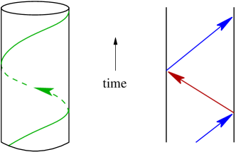
Figure 1: The edge modes with spacetime a cylinder (illustrated on the left) have only one chirality. The physics of these is closely related to that of a non-chiral system with spacetime a strip (illustrated on the right), where the boundary conditions couple the left and right movers.

To motivate our definition of the entropy, we first discuss a closely-related system, a non-chiral rational conformal field theory with boundaries. This means that spacetime at zero temperature is a strip of width $\pi R$ instead of a cylinder. At non-zero temperature, spacetime becomes a finite-width cylinder with period $\beta$ in the Euclidean time direction, instead of a torus. The left and right movers on the strip are coupled by the boundary conditions, as illustrated schematically in figure 1. This means the chiral and antichiral conformal symmetries are also coupled. Conformal invariance is preserved only with certain boundary conditions, and even then, only a single algebra remains Cardy84 . This symmetry algebra is exactly the same as that of a single chiral theory. The partition function for the model on the strip is then a sum over characters of a single algebra. These characters are exactly those in (16), and the partition function takes the same form (17), with $N_{a}$ integer Cardy86b ; Cardy89 .

The connections between the chiral theory on the cylinder and the non-chiral theory on the strip go even deeper. The boundary conditions which preserve conformal invariance are in one-to-one correspondence with the primary fields of this chiral rational conformal field theory, so each can be labeled by the same indices we use to label primary fields. (More precisely, conformal boundary conditions form a vector space, basis vectors of which can be labeled by the primary fields.) Then a key result of Cardy’s is that with appropriate regularization, the partition function $Z_{jk}$ on the strip with boundary conditions $j$ and $k$ at the two ends is Cardy89

$$Z_{jk}=\sum_{a}N^{a}_{jk}\chi_{a}(q)$$ (20)

where $N^{a}_{jk}$ is the same $N^{a}_{jk}$ which appears in the fusion rules! Furthermore, by using the Verlinde formula it is simple to find boundary conditions which result in a partition function given by a single character $\chi_{a}$.

These results were used by Affleck and Ludwig to define and compute what they called the “boundary entropy”Affleck91 . Consider an RCFT on the finite-width cylinder with boundary conditions $j$ and $k$, so that the partition function is $Z_{jk}$. Then take the width of the cylinder $R\to\infty$ while holding the temperature, and hence the radius $\beta$ of the cylinder, fixed at some non-zero finite value. Then, on general grounds, one must have

$$\ln{Z_{jk}}=fR+\ln(g)+\dots$$ (21)

where we neglect terms that vanish as $R\to\infty$. This is precisely the form (4). We can compute $f$ and $g$ by using a modular transformation, because the limit $R/\beta\to\infty$ corresponds to $\widetilde{q}=0$. From (18) we have

$$Z_{jk}=\sum_{a,b}N^{a}_{jk}S_{a}^{b}\chi_{b}(\widetilde{q}).$$

By definition, in this limit, the character $\chi_{a}$ behaves as

$$\lim_{\widetilde{q}\to 0}\ln\chi_{a}=\frac{2\pi R}{\beta}\left(\frac{c}{24}-h_{a}\right)$$

So unless $j$ and $k$ are such that $\sum_{a}N^{a}_{jk}S_{a}^{0}=0$, the identity character $\chi_{0}$ dominates and one has

$$f=\frac{\pi c}{12\beta},\quad\qquad g=\sum_{a}N^{a}_{jk}S_{a}^{0}.$$ (22)

It is then natural to interpret $g$ as a ground-state degeneracy, and $\ln(g)$ as a boundary entropy, since clearly this subleading term in the full entropy depends on the boundary conditions $j$ and $k$. However, $g$ is not necessarily an integer, so as we discussed in the introduction, it cannot, strictly speaking, be a ground-state degeneracy. Neither is it solely associated with the boundaries of the strip, since there is no particular reason that subleading terms from the 1$+$1 dimensional bulk cannot contribute to $\ln(g)$.

We now return to studying topological theories whose edge modes are described by chiral conformal field theories on the torus. Although the torus has no boundaries, there are still boundary conditions on the fields. For example, in the $p+ip$ superconductor, the edge fermions have antiperiodic or periodic boundary conditions around the spatial cycle of the torus depending on whether there are an even or an odd number of vortices in the two-dimensional bulk. So let us first consider the case where there are no bulk quasiparticles. In the language of topological field theory, this corresponds to trivial topological charge on the disk. The partition function of the edge RCFT is then

$$Z_{0}=\chi_{0}(q)$$

where, as above, the $0$ label on $\chi_{0}$ means the identity sector. To extract the piece of interest from this, we take the same $R/\beta\to\infty$ limit. $Z_{0}$ then can be expanded in the form (21), i.e.

$$\ln(Z_{0})=f_{0}R+\ln(\gamma_{0}),$$ (23)

where $\gamma$ in this chiral theory is the analog of the $g$ in (21) in the impurity theory. Following through the same modular transformation described in the preceding paragraph, we obtain the subleading contribution to $\ln(\chi_{0})$ in this limit:

$$\gamma_{0}=N_{00}^{0}S_{0}^{0}=S_{0}^{0}.$$

Recall, however, that we showed in (15) that $S_{0}^{0}=1/{\cal D}$, where ${\cal D}$ is the quantum dimension we have gone to great lengths to compute. We thus conclude

$${\cal S}_{\hbox{edge}}\equiv\ln(\gamma_{0})=-\ln({\cal D})$$ (24)

as the universal part of the edge entropy. There is no particular reason for $\gamma_{0}$ to be an integer, since it is a subleading term in the large $R/\beta$ expansion.

Note that ${\cal S}_{\hbox{edge}}$ is identical to the universal piece of the topological entanglement entropy in (3). Although the two quantities are defined in different ways, this is hardly a coincidence. ${\cal S}_{\hbox{edge}}$ is defined for a system with a real edge, while the topological entanglement entropy is defined on the boundary between two regions $A$ and $B$, not a physical edge. Nevertheless, one expects the two to be the same. Edge modes arise formally in a topological theory to cancel the chiral anomaly Wen91 . The topological entanglement entropy arises formally by integrating out the system beyond the boundary, i.e. subsystem $B$. When integrating out the degrees of freedom of $B$, one of course integrates out an anomaly-free theory, so this must include the edge modes of $B$ as well. The remaining $A$ theory then, in some sense, must include “edge modes” as well which are required to cancel those on $B$. This required cancellation is one way of seeing that systems $A$ and $B$ are indeed entangled. Thus, the value of the topological entanglement entropy should be identical to our computation of the edge entropy. We have shown by direct computation that this is indeed the case.

IV.2 Bulk entanglement entropy

The correspondence between thermodynamic and entanglement entropies goes much deeper. Let us now consider the bulk entanglement entropy. This arises in non-abelian topological phases because of multiple possible fusion channels. For example, two vortices in a $p+ip$ superconductor form a two-state quantum system, so their entanglement entropy is $\ln(2)$.

We can derive a simple formula for the bulk entanglement entropy in general. We define the topological degeneracy of a given state to be the number of ways one can fuse the quasiparticles present to get a particular overall fusion channel. This is easily written in terms of the matrix $Q_{a}$ defined in (12). When there are $n_{a}$ of each of the quasiparticles labeled by $a$, define the matrix $T$ by

$$T=\prod_{a}(Q_{a})^{n_{a}}$$ (25)

It makes no difference in which order we multiply the $Q_{a}$ because different $Q_{a}$ commute with each other (as we showed from the Verlinde formula, they have the same eigenvectors). The topological degeneracy of channel $c$ is then the $c,0$ entry of this matrix $T$. Note that this is a simple generalization of the way we computed the quantum dimension to the case in which different types of particles are allowed to be present.

Let us illustrate this in terms of the $p+ip$ superconductor, where there are three states in the topological field theory, labeled by $I$, $\psi$ and $\sigma$. If there are no bulk quasiparticles present, we have degeneracy $1$ in the identity channel. If we have only $\psi$ quasiparticles, the fusing is simple: for an even number of $\psi$ quasiparticles the degeneracy is $1$ in the identity channel, while for an odd number the degeneracy is $1$ in the $\psi$ channel. It gets more interesting for bulk $\sigma$ quasiparticles. A single bulk $\sigma$ quasiparticle corresponds to degeneracy $1$ in the $\sigma$ channel. However, two bulk $\sigma$ quasiparticles does not correspond to degeneracy $2$. Since $\sigma\cdot\sigma=I+\psi$, two bulk $\sigma$ quasiparticles corresponds to degeneracy $1$ in both the $I$ channel and in the $\psi$ channel. Degeneracy $2$ in the $\sigma$ channel occurs for three bulk $\sigma$ quasiparticles. In general, for an even number $2M$ of bulk $\sigma$ quasiparticles, we have degeneracy $2^{M-1}$ in the $I$ and $\psi$ channels while for an odd number $2M+1$, we have degeneracy $2^{M}$ in the $\sigma$ channel. Including any number of $\psi$ quasiparticles doesn’t change the degeneracies (except for $M=0$).

The bulk entanglement entropy arises from the uncertainty in knowing which quantum state the bulk quasiparticles are in. For example, if there are two bulk $\sigma$ quasiparticles, we do not know without doing a measurement whether they are in the $I$ or $\psi$ channel. The entropy is therefore $\ln(2)$. But what if there is just one $\sigma$ quasiparticle in a region? It can be entangled with a $\sigma$ quasiparticle in another region of the droplet, giving a total entropy of $\ln(2)$. Since entropy is additive, the only consistent possibility is for the single $\sigma$ quasiparticle to have entropy $\ln(\sqrt{2})$. In general, a single quasiparticle of type $a$ has entropy $\ln(d_{a})$, where $d_{a}$ is the quantum dimension discussed at great length above. The general expression for the bulk entropy can be expressed easily in terms of the topological degeneracies, namely

$${\cal S}_{\hbox{bulk}}=\ln\!\biggl{(}\sum_{c}T_{0c}{d_{c}}\biggr{)}\ .$$ (26)

This can be simplified by rewriting $d_{c}$ and $T_{c0}$ in terms of the modular $S$ matrix. We can use the Verlinde formula (13) for $Q$ and the relation $d_{c}=S_{c}^{0}/S_{0}^{0}$. The latter is the eigenvector of any $Q_{a}$, having eigenvalue $S^{0}_{a}/S_{0}^{0}=d_{a}$. Thus it is an eigenvector of $T$ as well, so

$${\cal S}_{\hbox{bulk}}=\sum_{a}n_{a}\ln(d_{a})\ .$$ (27)

Each quasiparticle of quantum dimension $d_{a}$ contributes $\ln(d_{a})$ to the bulk entanglement entropy. Note that this “bulk” entropy is extensive not in the size of the sample, but rather in the number of bulk quasiparticles.

IV.3 The bulk and edge entropies from the holographic partition functions

We show here that the entire topological entanglement entropy can be seen in terms of the edge conformal field theory. We interpret this as an example of holography. In a topological field theory, the degrees of freedom live on the edge. In the fractional quantum Hall effect, these are, of course, the edge modes we have been discussing all along. Holography simply means that all the information of the bulk topological field theory is encoded in the edge modes.

As we have discussed above, adding or removing bulk quasiparticles changes the boundary conditions on the edge modes. This will change the chiral partition function for the edge. To illustrate this, consider the $p+ip$ superconductor, where there are three characters: $\chi_{I}$, $\chi_{\psi}$ and $\chi_{\sigma}$, with a modular $S$ matrix given in (32). The presence of $\sigma$ quasiparticles (the vortices) in the bulk has an important effect on the edge. As we reviewed in ref. Fendley06b, , an odd number of $\sigma$ quasiparticles changes the boundary conditions of the edge Majorana fermion from antiperiodic around the circle to periodic. For a fermion with periodic boundary conditions on the 1$+$1 dimensional torus, the chiral partition function is $\chi_{\sigma}$. Thus we define the holographic partition function for a single bulk $\sigma$ quasiparticle to be $Z_{\sigma}=\chi_{\sigma}.$ This partition function yields the correct entanglement entropy. Taking the $L/\beta\to\infty$ limit as in (23) yields

$$\gamma_{\sigma}=S_{I}^{\sigma}=\frac{1}{\sqrt{2}}.$$

For a $p+ip$ superconductor with one vortex in region $A$, the entanglement entropy is indeed

$${\cal S}_{\hbox{bulk}}+{\cal S}_{\hbox{edge}}=\ln(\sqrt{2})-\ln(2)=-\ln(\sqrt{2}).$$

We define the holographic partition function for a single bulk $\psi$ quasiparticle in a similar fashion: $Z_{\psi}=\chi_{\psi}$. The corresponding entropy is then $\ln(S^{\psi}_{I})=\ln(1/2)=-\ln{\cal D}$. This is just ${\cal S}_{\hbox{edge}}$, which is indeed what we expect, because there is no bulk topological entropy for $\psi$ quasiparticles.

Given our definition of the bulk entanglement entropy, it should be obvious how to define the holographic partition function for an arbitrary number of bulk particles. The effect of adding a bulk quasiparticle is given by the same fusion rules as for the primary fields. For example, in the $p+ip$ superconductor, the fusion rule $\psi\cdot\psi=I$ means that with no $\sigma$ quasiparticles and an even (odd) number of $\psi$ quasiparticles, we define the holographic partition function to be $\chi_{I}$ ($\chi_{\psi}$). In both cases the entropy remains $-\ln{\cal D}$, since there is no bulk entanglement entropy. A less trivial case is when we have two bulk $\sigma$ quasiparticles. Here the holographic partition function follows from the fusion rule $\sigma\cdot\sigma=I+\psi$, so we get

$$Z_{2\sigma}=\chi_{I}+\chi_{\psi}.$$

For three, the topological degeneracy is $2$ in the $\sigma$ channel, so we get

$$Z_{3\sigma}=2\chi_{\sigma},$$

and so on.

The definition of the holographic partition function for arbitrary numbers of quasiparticles in the bulk should now be obvious. In general, for $n_{a}$ bulk quasiparticles of each type $a$, the holographic partition function is

$$Z=\sum_{a}T_{0a}\chi_{a}(q)$$ (28)

where $T$ is the topological degeneracy matrix defined in (25). This is the partition function obtained by computing the path integral for the appropriate 2$+$1 dimensional topological field theory (e.g. Chern-Simons theory) with spacetime $D\times S_{1}$, where $D$ is a disk of radius $R$, and $S_{1}$ a circle of radius $\beta$. To get the correct degeneracies $T_{0a}$ one needs to insert $n_{a}$ Wilson loops of each type $a$ which puncture the disk and wrap around the $S_{1}$.

As advertised, the holographic partition function (28) gives the correct entanglement entropy in the the $R/\beta\to\infty$ limit. In this limit,

$$Z=\sum_{a}T_{0a}S_{a}^{0}\chi_{0}(\widetilde{q})+\dots\ .$$

We define the total thermodynamic entropy ${\cal S}$ via our usual expansion

$$\ln(Z)=fR+{\cal S}+\ldots\ .$$

Using $d_{b}=S^{b}_{0}/S_{0}^{0}$ along with the expressions for the bulk and edge entropies (26) and (27) gives

$${\cal S} = \ln(\sum_{a}T_{0a}S_{a}^{0})$$ (29)

$$= \ln(\sum_{a}T_{0a}d_{a})+\ln(S_{0}^{0})$$

$$= \sum_{a}n_{a}\ln(d_{a})-\ln({\cal D})\ .$$

Thus we see that indeed once we have taken the $R/\beta\to\infty$ limit, we have

$${\cal S}={\cal S}_{\hbox{bulk}}+{\cal S}_{\hbox{edge}}\ .$$ (30)

The holographic partition includes both bulk and edge entanglement entropies.

We close this section by returning to where it started, a discussion of the relation between chiral conformal field theory with spacetime a torus and non-chiral conformal field theory on a finite-width cylinder. The partition functions in both cases are expressed in the form

$$Z=\sum_{a}N_{a}\chi_{a}$$

where the $N_{a}$ are integers, describing how many times each character appears. In the latter case, however, there is one important restriction which we need not demand of the holographic partition function. For a partition function describing a unitary field theory on the finite-width strip with physical boundary conditions, the identity character usually appears at most once (i.e. $N_{0}=0$ or $1$). The reason is that there is only one identity field in a unitary theory, so only with peculiar boundary conditions can one have $N_{0}>1$. In the holographic partition function, $N_{0}$ can be any non-negative integer: it is the number of ways the bulk quasiparticles in the 2$+$1 dimensional topological theory can fuse to get the identity channel. Thus although the partition functions are defined in a very similar fashion, they really are different objects.

V Dynamical Entropy Loss at a Point Contact

The relation between the thermodynamic and entanglement entropies manifests itself most dramatically through the dynamics of a point contact connecting two points on the boundary of the disk. Quasiparticles can tunnel between the two points connected by the contact, thereby perturbing the edge modes at these two points. This can change the edge entropy. When the tunneling operator is a relevant perturbation, it causes the system to flow to an infrared fixed point at which any edge excitation which is incident upon the contact necessarily tunnels across the system. In other words, an imaginary boundary between the two halves evolves dynamically into a real edge. As we shall see below, this process causes the entanglement entropy between the two halves to be, in a sense, “reborn” as the actual thermodynamic entropy of the two resulting droplets. We have discussed a point contact in a non-abelian topological state in depth in a companion paper Fendley06b , and the results in this section complement those results.

As mentioned in the introduction, if we compute the density matrix for half of a system by tracing out the degrees of freedom of the other half, the resulting density matrix has an entanglement entropy

$${{\cal S}_{A}}=aL-\ln{\cal D}+\ldots$$

The second, universal term is negative. What it tells us is that there is a little less uncertainty in the state of half of the system than one might have naively expected purely from local correlationsKitaev05 ; Levin05 . A priori, this has absolutely nothing to do with the thermodynamic entropy of the system since it is obtained from an arbitrary division of the ground state wavefunction alone, with nothing about the spectrum taken into account. However, when the strong tunneling fixed point is reached, the disk is effectively split into two. The imaginary division into two halves becomes a real division. Entropy is lost as a result of this process because the edge entropy for two disks is $-2\ln({\cal D})$, compared to $-\ln({\cal D})$ for a single disk. As in the case of the entanglement entropy, this extra negative contribution is due to the fact that we know more about the system: the negative contribution $-\ln({\cal D})$ to the entropy of a disk represents the information that we know about the system when we know that it has trivial total topological charge. However, one half of the system could have arbitrary topological charge $a$, so long as the other half has the compensating topological charge $\bar{a}$. If the point contact breaks the system into two systems, each with trivial topological charge, then this uncertainty is lost. The information which we now know about the two disks is $-2\ln({\cal D})$.

Defining ${\cal S}_{UV}$ to be the entropy in the limit in which there is no tunneling across the sample (the UV limit), and ${\cal S}_{IR}$ to be the entropy in the limit in which tunneling is strong (the IR limit), we have

$${\cal S}_{UV}-{\cal S}_{IR}=-\ln({\cal D})-(-2\ln({\cal D}))=\ln({\cal D})\ .$$ (31)

Here, we have assumed that there are no quasiparticles in the bulk, and that the system breaks into two halves each with no quasiparticles. However, the entropy change is the same even when quasiparticles are present, which we will discuss below.

Let us first illustrate entropy loss due to a point contact in the abelian case, when the edge theory consists of a free boson. This has been widely studied in the context of the Laughlin fractional quantum Hall states Kane92 . By using a series of mappings, the chiral problem on the torus can be shown to be exactly equivalent to a non-chiral problem on the finite-width cylinder. In other words, the analogy we made in the previous section is an exact equivalence in this case. The point contact results in a boundary with Neumann boundary conditions on the boson in the UV limit, and Dirichlet boundary conditions in the IR Wong94 . The edge entropies can be computed in both cases, and one obtains Wong94 ; Fendley94 for $\nu=1/m$

$${\cal S}_{UV}-{\cal S}_{IR}=\ln(\sqrt{m}).$$

This is exactly what one obtains from our results by assuming that the IR limit consists of two separate disks. We show in (37) that ${\cal D}=\sqrt{m}$ for the $\nu=1/m$ Laughlin states. Thus we indeed have ${\cal S}_{UV}-{\cal S}_{IR}=\ln({\cal D})$ as in (31).

Using the results derived above, we can check (31) in several non-abelian cases. As we showed in ref. Fendley06b, , a point contact in the $p+ip$ superconductor is equivalent to the single-channel anisotropic Kondo problem. The entropy change is well-known here. The Kondo problem consists of a single impurity spin antiferromagnetically coupled to an electron gas. In the single-channel spin-1/2 case, the spin is decoupled in the UV limit, while it is completely screened in the IR limit. Therefore ${\cal S}_{UV}=\ln(2)$, while ${\cal S}_{IR}=\ln(1)=0$. We showed in (8) that for the Ising model, ${\cal D}_{p+ip}=2$, so (31) holds.

A point contact in the Moore-Read Pfaffian state at $\nu=1/2$ (or $\nu=5/2$) turns out to be a variant of the two-channel overscreened Kondo problem. In ref. Fendley06a, , we showed that the entropy loss here is ${\cal S}_{UV}-{\cal S}_{IR}=2\ln(\sqrt{2})$. In (41), we show that ${\cal D}_{MR}=2\sqrt{2}$, so again (31) holds. For a point contact in a Read-Rezayi state or for $SU(2)_{k}$ for general $k$, it is not yet known how to map the tunneling operator onto a Kondo-like problem, so we do not have an independent result against which to check the prediction which can be obtained from (31) along with the quantum dimension in (44).

The entropy change (31) can also be seen in terms of the holographic partition functions. The partition function for two independent systems is simply the product of the partition functions for the two systems. Thus when the point contact splits the system into two, the holographic partition function should be the product of two holographic partition functions. Let us first examine this in the case where there are no bulk quasiparticles. In the IR limit, the system decouples into two independent discs, each with no bulk quasiparticles. Thus the partition function is $Z_{0}=\chi_{0}(q)$ for the UV, and

$$Z_{0,0}=\chi_{0}(q_{1})\chi_{0}(q_{2})$$

for the IR. We have denoted $q_{1}=\exp(-2\pi\beta/R_{1})$ and $q_{2}=\exp(-2\pi\beta/R_{2})$, where $R_{1}$ and $R_{2}$ are the sizes of the discs into which the point contact splits the system in the IR limit. The universal piece of the entropy extracted from $\chi_{a}(q)$ is independent of how $q$ is taken to 1, so we obtain entropies of $-\ln({\cal D})$ for the entropy associated with each of the two disks. Thus from $Z_{0,0}$ we obtain ${\cal S}_{IR}=-2\ln({\cal D})$, as required.

When there are bulk quasiparticles, they must end up on one side or the other once the disk is split. The UV holographic partition function for a quasiparticle of type $a$ is denoted $\chi_{a}(q)$, which from (29) gives the entanglement entropy of ${\cal S}_{UV}=\ln(d_{a})-\ln({\cal D})$. When there is one bulk quasiparticle, it must end up on one half or another, but it cannot end in both. There are therefore two possibilities for the IR partition function:

$$Z_{a,0}=\chi_{a}(q_{1})\chi_{0}(q_{2}),\qquad\hbox{ or }\qquad Z_{0,a}=\chi_{0}(q_{1})\chi_{a}(q_{2}).$$

We cannot predict which one is realized, but one or the other will happen. Either of the two yields the correct entanglement entropy

$${\cal S}_{IR}=\ln(d_{a})-2\ln({\cal D}).$$

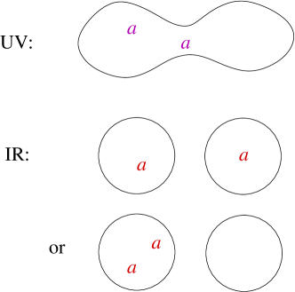
Figure 2: In the UV, bulk quasiparticles can be anywhere. In the IR, they must end up on one of the two sides. For two bulk quasiparticles of type $a$, they can both end up on one side, or on separate sides.

For multiple particles, we must apply the fusion rules just as we did for the UV holographic partition functions. For two quasiparticles of type $a$, there are three possibilities for how they might end up, as illustrated schematically in figure 2. If one quasiparticle ends up on each disk, then the IR holographic partition is $Z_{a,a}=\chi_{a}(q_{1})\chi_{a}(q_{2}).$ If both quasiparticles end up on the same disk, then e.g.

$$Z_{2a,0}=Z_{2a}(q_{1})Z_{0}(q_{2})=\left(\sum_{b}N_{aa}^{b}\chi_{b}(q_{1})\right)\chi_{0}(q_{2}).$$

For example, for the $p+ip$ superconductor with two bulk $\sigma$ quasiparticles, we have

$$Z_{2\sigma,0} = (\chi_{I}(q_{1})+\chi_{\psi}(q_{1}))\chi_{I}(q_{2}),$$

$$Z_{\sigma,\sigma} = \chi_{\sigma}(q_{1})\chi_{\sigma}(q_{2}).$$

Thus the general rule is simple: for a given subdivision, the holographic partition on each half is the same as it would be for an isolated disc. Then multiply the characters for the two separated halves together.

With this holographic partition for the IR, the bulk part of the entropy remains $\sum_{a}n_{a}\ln(d_{a})$ in the IR. It does not matter which half the bulk quasiparticle is on: it still contributes $\ln(d_{a})$ in accord with the intuition that a point contact should not affect the bulk of the sample. As we have seen in (31), the edge entropy changes, doubling from $-\ln({\cal D})$ to $-2\ln({\cal D})$.

VI Discussion

The ideas presented here grew out of our attempts to understand quasiparticle tunneling at a point contact in a Moore-Read Pfaffian non-Abelian quantum Hall state Fendley06a ; Fendley06b . A key technical challenge in this problem was to formulate a bosonized description of the tunneling of twist fields (or Ising spin fields) $\sigma$ between Majorana fermion edge modes. We found that this could be done if one introduced a spin-$1/2$ degree of freedom at the point contact which served a ‘bookkeeping’ purpose of keeping track of how many $\sigma$ fields had tunneled. We thereby saw that the tunneling Hamiltonian for this problem could be mapped onto various versions (depending on filling fraction of the quantum Hall state) of the Kondo model. Therefore, the issue of entropy loss due to the point contact was inescapable, although the same issue arises in simpler cases such as Abelian quantum Hall states but could be ignored there. Our interpretationFendley06a , on which we have elaborated here, is that this entropy loss cannot be ascribed to the point contact per se. Rather, it should be understood as a $(2$+$1)$-dimensional entanglement entropy. When tunneling at a point contact causes a Hall droplet to be effectively broken in two, the topological entanglement entropy between the two sides becomes actual thermodynamic entropy. Since this entropy is negative, ${\cal S}=-\ln{\cal D}$, the entropy of the system decreases.

One implication of our results is that an attempt to formulate a tractable representation of tunneling in other non-Abelian quantum Hall states, such as the Read-Rezayi states, will require introducing an ‘impurity’ degree of freedom at the point contact, analogous to the Kondo spin in the Moore-Read Pfaffian case, to give us the correct entropy loss.

It would be interesting to see which of these results apply to gapless 2$+$1 dimensional theories in a topological phase. Such theories are often closely related to conformal field theories, but these theories are not describing the edge modes, but rather the behavior in two-dimensional space. The entanglement entropy for such systems Fradkin06 is quite similar to the entropies discussed here, and it would be interesting to pursue the analogies further.

It would also be interesting to explore the connection of these results with those motivated by gauge theory, string theory, and black holes. Results quite analogous to ours have been derived using the AdS/CFT correspondence Ryu06 . The conformal field theories here are simpler than those which generally arise from the AdS/CFT correspondence (ours are unitary and rational), and it would be interesting to understand how quantum Hall physics fits into this more general setting.

Acknowledgments  We would like to thank J. Cardy, E. Fradkin, M. Freedman, A. Kitaev, A. Ludwig, J. Preskill, and N. Read for discussions. This research has been supported by the NSF under grants DMR-0412956 (P.F.), PHY-9907949 and DMR-0529399 (M.P.A.F.) and DMR-0411800 (C.N.), and by the ARO under grant W911NF-04-1-0236 (C.N.).

Appendix A Examples of Quantum Dimensions

A.1 Ising model/$p+ip$ superconductor

The Ising conformal field theory is equivalent to a free massless Majorana fermion. The partition function on the torus – and hence the characters of interest – can be computed using the properties of free fermions; the main subtlety is that to compute characters for all the primary fields $I,\psi,\sigma$ one needs to utilize both periodic and antiperiodic boundary conditions on the fermion. The connection between the different characters and the different boundary conditions is reviewed in depth in, for instance, ref. Ginsparg89, . In the $p+ip$ superconductor, inserting a $\sigma$ quasiparticle (i.e. a vortex) in the bulk flips the boundary conditions on the fermion between periodic and antiperiodic around the disk (see e.g. ref. Fendley06b, ).

It is natural and convenient to write conformal-field-theory characters in terms of Jacobi theta functions. The behavior of theta functions under modular transformations is simple, so it is then straightforward to work out the modular $S$ matrix. Explicit expressions for the characters can be found in Refs. Cardy86a, ; Ginsparg89, . The modular $S$ matrix for the Ising model is Cardy86a

$${S}_{\rm Ising}=\begin{pmatrix}\frac{1}{2}&\frac{1}{2}&\frac{1}{\sqrt{2}}\\ \frac{1}{2}&\frac{1}{2}&-\frac{1}{\sqrt{2}}\\ \frac{1}{\sqrt{2}}&-\frac{1}{\sqrt{2}}&0\end{pmatrix}$$ (32)

where we write the fields in the order $I,\psi,\sigma$. Note that $S^{2}=1$, as required.

Using (14), we find $d_{I}=1$, $d_{\psi}=1$ and $d_{\sigma}=\sqrt{2}$, as we saw directly from the fusion rules. Using (15), we find the total quantum dimension ${\cal D}_{p+ip}=2$, as we saw in (8).

A.2 Free boson/Laughlin states

Before studying the non-abelian Moore-Read Pfaffian state, it is first useful to study the abelian Laughlin state at $\nu=1/3$. The latter is the first state in the a sequence of quantum Hall states, with the Moore-Read Pfaffian second. The quasiparticles and quasiholes in the Laughlin state at $\nu=1/3$ are abelian anyons, with charges $\pm 1/3$.

The conformal field theory describing the edge modes of the Laughlin states is simply a free chiral boson $\varphi(z)$ Wen91 . Here (and in most situations of interest), the boson is compact, meaning in our chiral context that operators must be invariant under the shifting $\varphi(z)$ to $\varphi(z)+2\pi r$ for some “radius” $r$ (not to be confused with the radius $R$ of the disk; calling $r$ a radius is a relic of string theory). Then standard manipulations show that a free boson has central charge $c=1$, and that the primary fields on the punctured plane under conformal symmetry are Ginsparg89

$$V_{\gamma}(z)\equiv e^{i\gamma\varphi(z)},\qquad\qquad\gamma=\frac{n}{r}$$ (33)

for integer $n$. The operator $e^{i\gamma\varphi}$ appears frequently in the Coulomb-gas approach to $2d$ statistical mechanical models, and in string theory as a vertex operator.

With the conventional normalization of $\varphi$, $V_{\gamma}$ has scaling dimension $\gamma^{2}/2$. This means that the eigenvalue of ${\cal H}$ acting on the state created by $V_{\gamma}$ is $2\pi(\gamma^{2}/2-1/24)/R$. More standard calculations show that the operator product expansion is

$$e^{i\gamma\varphi(z)}e^{i\delta\varphi(w)}=(z-w)^{\gamma\delta}e^{i\gamma\varphi(z)+i\delta\varphi(w)}.$$ (34)

To obtain correlation functions on the cylinder, it is usually most convenient to first work them out on the punctured plane, and then conformally transform them to the cylinder. In general, a primary field $\Phi(z,\overline{z})$ of dimensions $(h,\overline{h})$ transforms under the conformal transformation $z^{\prime}=f(z)$ as (again, see e.g. Ginsparg89 )

$$\Phi(z,\overline{z})\to\left(\frac{\partial{f}}{\partial{z}}\right)^{{h}}\left(\frac{\partial\overline{f}}{\partial\overline{z}}\right)^{\overline{h}}\Phi\left(f(z),\overline{f}(\overline{z})\right).$$

For the transformation from the punctured plane to the cylinder, we have $\tau+i\sigma=R\ln(z)/2\pi$, so for the operators $V_{\gamma}(z)$, we have

$$V_{\gamma}(z)\to\left(\frac{R}{2\pi z}\right)^{\gamma^{2}/2}V_{\gamma}(\tau+i\sigma).$$ (35)

The fact that there is only one primary field on the right-hand-side of the operator product expansion (34) means that the quantum dimension of all the operators $V_{\gamma}$ are $d_{\gamma}=1$. Computing the total quantum dimension ${\cal D}$ for a free boson is more work, because there are an infinite number of primaries if we use only conformal symmetry since the operator product expansion for $N$ operators $V_{\gamma}$ gives the operator $V_{N\gamma}$. One interesting symmetry generator is the $U(1)$ current $\partial_{z}\varphi$. In the fractional quantum Hall effect, this is the electrical charge current. To define ${\cal D}$, we must find the largest possible symmetry algebra. For any rational $r^{2}$, one can extend the symmetry algebra by some integer-dimension operator and obtain a finite number of primary fields, thus giving a rational conformal field theory.

However, for the $\nu=1/m$ Laughlin states in the fractional quantum Hall effect, the extended symmetry is even larger. As we discussed above, one needs to extend the algebra by the electron annihilation/creation operators. These have dimension $m/2$ Wen91 . A field with half-integer dimension is fermionic; symmetries with such generators occur for example in the Gross-Neveu model for an odd number of Majorana fermions Witten78 . (Incidentally, in these Gross-Neveu models, the massive quasiparticles end up having a quantum dimension of $\sqrt{2}$. Fendley02 ) For the simplest non-trivial case $m=3$, the generators are of dimension 3/2. The symmetry here is supersymmetry Milovanovic96 . It is called ${\cal N}=2$ supersymmetry, because there are two generators: the electron creation and annihilation operators. The entire sequence of Read-Rezayi states Read99 , of which the $\nu=1/3$ Laughlin state is the first member and the Moore-Read state the second, has ${\cal N}=2$ supersymmetry as its extended symmetry.

Using the operator product expansion, it is simple to see what the primary fields are for the $\nu=1/3$ Laughlin state. The supersymmetry generators are $G^{\pm}=e^{\pm i\sqrt{3}\varphi}$, which indeed have dimension $3/2$ and charge $\pm 1$. From (34), we have

$$G^{\pm}(z)V_{\gamma}(w)=(z-w)^{\pm\sqrt{3}\gamma}V_{\gamma\pm\sqrt{3}}(w)\left(1\ +\ \dots\right)$$ (36)

where the terms omitted are regular in $z-w$. The transformation rule (35) means that when $G^{\pm}(z)$ is transformed from the punctured plane to the cylinder, it is multiplied by a factor of $z^{3/2}$. Thus the antiperiodicity of the electron/supersymmetry generators on the cylinder means that they are periodic on the punctured plane. Since we are only interested in this sector, the primary fields are those for which the exponent of the $(z-w)$ piece in (36) is an integer. The lowest non-zero value of $|\gamma|$ for which this is true is $\gamma=1/\sqrt{3}$, so we must have $r=1/\sqrt{3}$. Thus the allowed operators $V_{\gamma}$ here must have $\gamma=n/\sqrt{3}$ for integer $n$. In this language, the supersymmetry generators themselves correspond to $n=\pm 3$. Thus the only primary fields under the extended algebra have $n=0$ (the identity field), and $n=\pm 1$ (which have dimension $1/6$). The remaining values of $n$ can be obtained by acting with $G^{\pm}$ on these three primaries, as is clear from the operator product expansion (36). For example, one obtains $V_{2/\sqrt{3}}$ by acting with $G_{+}$ on $V_{-1/\sqrt{3}}$. Physically, this means that all the edge modes can be obtained from these three by attaching a hole or an electron. There are thus three types of quasiparticles in the Laughlin state at $\nu=1/3$, so ${\cal D}_{1/3}=\sqrt{3}.$ For general integer $m=1/\nu$, the extended symmetry generator is $V_{\sqrt{m}}$, so by the same type of argument, one finds $m$ primary fields. This yields

$${\cal D}_{\nu=1/m}=\sqrt{m}$$ (37)

as noted in the introduction.

One important subtlety to note is that this is the sector of the theory corresponding to antiperiodic boundary conditions around the cylinder for fermionic fields such as the supersymmetry generator. In the language of supersymmetry, this is called the Neveu-Schwarz sector. As we noted previously, periodic boundary conditions on fermions in an edge theory arise from a vortex in the bulk. Fields local with respect to a supersymmetry generator with periodic boundary conditions are in the Ramond sector. In an ${\cal N}=2$ supersymmetric theory, there must be the same number of primary fields in the Ramond sector as the Neveu-Schwarz sector, so ${\cal D}$ remains the same. For the boson with $r=1/\sqrt{3}$, the fields $V_{n/\sqrt{3}}$ for half-integer $n$ are local with respect to $G_{\pm}$ with periodic boundary conditions. The Ramond primaries are then those with $n=\pm 1/2$ and $n=3/2$, so ${\cal D}$ indeed remains $\sqrt{3}$. Note that $n=-3/2$ is not a primary because it can be obtained by acting on $V_{\sqrt{3}/2}$ with $G_{-}$.

Models with non-abelian statistics need not have $d_{a}=1$ like the free boson does. Thus one needs to work out the fusion algebra, which is simplest to do by using the modular $S$ matrix. Since many interesting models (e.g. all models of the fractional quantum Hall effect) involve a free boson, we display here the characters for the free boson. This also will provide a check on the above result for ${\cal D}$.

For a free boson, the highest-weight states under the symmetry algebra including the $U(1)$ current $\partial\varphi$ are created by the primary fields $V_{\gamma}$ defined in (33). The highest-weight state created by $V_{\gamma}$ has dimension $\gamma^{2}/2$, so the leading term in the character must have exponent $\gamma^{2}/2-1/24$. The full characters with this symmetry algebra are (see e.g. Ref. Ginsparg89, )

$$\chi_{\gamma}(q)=\begin{cases}\frac{q^{\gamma^{2}/2}}{\eta}\qquad\quad&\gamma\neq p/\sqrt{2}\\ \frac{q^{p^{2}/4}-q^{(p+2)^{2}/4}}{\eta}\qquad&\gamma=p/\sqrt{2}\\ \end{cases}$$ (38)

for $p$ integer. The denominator is the Dedekind eta function, which is defined as

$$\eta(q)\equiv q^{1/24}\prod_{n=1}^{\infty}(1-q^{n}).$$

Its key property is that when $q^{-1/24}\eta$ is expanded in powers of $q$, the coefficient of $q^{m}$ is the number of partitions of $m$, i.e. the number of ways $m$ can be written as the sum of positive integers. This often occurs in characters, because descendant states are given by acting on primary states with the $L_{-n}$s for $n$ a positive integer.

The characters for the symmetry algebra extended to include supersymmetry are a sum over the characters $\chi_{m/\sqrt{3}}$, because the supersymmetry generators $V_{\pm\sqrt{3}}$ acting on $V_{m/\sqrt{3}}$ take it to $V_{(m\pm 3)/\sqrt{3}}$, as shown in (36). To avoid confusion with the Ising characters and with the $\chi_{\gamma}$, we denote the character in the identity sector here as $\chi[0]$, and those for the primaries with $m=\pm 1$ as $\chi[\pm 1/3]$. One then finds that

$$\chi[0] = \sum_{n=-\infty}^{\infty}\chi_{n\sqrt{3}}=\frac{J(q^{3})}{\eta}$$

$$\chi[\pm 1/3] = \frac{1}{2}\sum_{n=-\infty}^{\infty}(\chi_{n/\sqrt{3}}\ -\chi_{n\sqrt{3}})=\frac{J(q^{1/3})-J(q^{3})}{2\eta}$$

where we have defined

$$J(p)\equiv\sum_{n=-\infty}^{\infty}p^{n^{2}/2},$$

so that for small $p$, $J(p)=1+2p^{1/2}+2p^{2}+\dots$. It is a straightforward exercise to generalize these free-boson characters to the $\nu=1/m$ case, where the extended-symmetry generators are of dimension $m/2$.

To find the modular $S$ matrix, we need to rewrite the characters as functions of $\widetilde{q}$. Luckily, doing such modular transformations is a well-understood branch of mathematics. We have defined $J(p)$ as a special case of a Jacobi elliptic theta function. Then, from standard mathematical texts, one finds that

$$J(\widetilde{q}^{1/\Delta}) = (-\Delta\ln q/2\pi)^{1/2}J(q^{\Delta})\ ,$$

$$\eta(\widetilde{q}) = (-\ln q/2\pi)^{1/2}\eta(q)\ .$$ (39)

A little algebra then gives the modular transformations

$$\chi[0](\widetilde{q}) = \frac{1}{\sqrt{3}\eta(q)}J(q^{1/3})\ ,$$

$$\chi[\pm 1/3](\widetilde{q}) = \frac{\sqrt{3}}{2\eta(q)}J(q^{3})-\frac{1}{2\sqrt{3}\eta(q)}J(q^{1/3})\ .$$

We now need to rewrite the right-hand-side in terms of $\chi[0](q)$ and $\chi[\pm 1/3](q)$. We can exploit the equality $\chi[1/3](q)=\chi[-1/3](q)$ to find the modular $S$ matrix which is both symmetric and unitary. We find

$${S}_{\nu=1/3}=\begin{pmatrix}\frac{1}{\sqrt{3}}&\frac{1}{\sqrt{3}}&\frac{1}{\sqrt{3}}\\ \frac{1}{\sqrt{3}}&\frac{1}{2}-\frac{1}{2\sqrt{3}}&\ -\frac{1}{2}-\frac{1}{2\sqrt{3}}\\ \frac{1}{\sqrt{3}}&-\frac{1}{2}-\frac{1}{2\sqrt{3}}&\frac{1}{2}-\frac{1}{2\sqrt{3}}\end{pmatrix}$$

From this modular $S$ matrix we can read off the quantum dimensions $d_{a}=1$ for all three quasiparticles, and ${\cal D}=1/S_{0}^{0}=\sqrt{3}$, in agreement with our earlier results.

A.3 Moore-Read state

The edge theory for the $\nu=5/2$ Moore-Read state consists of a free boson (usually called the charge mode), and a Majorana fermion (usually called the neutral mode) Milovanovic96 . This conformal field theory has $c=3/2$. The edge electron/hole creation operators (i.e. the supersymmetry generators) are

$$G^{\pm}=\psi\,e^{\pm i\sqrt{2}\varphi}.$$

Because the fermion $\psi$ has dimension $1/2$, the generators have dimension $3/2$, and it is simple to show that as in the case of the $\nu=1/3$ Laughlin state, the extended symmetry is ${\cal N}=2$ supersymmetry.

The primaries of the combined field theory must be products of the primaries $I,\psi,\sigma$ of the Ising model with the primaries $V_{\gamma}$ for a free boson. The Ising primary fields have dimensions $0,1/2,1/16$ respectively, so by using the OPE (34) and the Ising fusion rules (II), it is simple to work out the powers of $z-w$ in the operator products in the combined theory. Demanding that the electron/superconformal generators be periodic on the punctured plane gives the primaries of the extended symmetry algebra to be

$$I,\ \sigma V_{\pm 1/(2\sqrt{2})},\ \psi,\ V_{\pm 1/\sqrt{2}}.$$ (40)

All primaries are all invariant under the combined transformations $\sigma\to-\sigma$, $\psi\to\psi$ and $\varphi\to\varphi+2\pi\sqrt{2}$; this is the condition that ensures locality. Fields that are odd under this symmetry comprise the Ramond sector.

We can compute the quantum dimensions without the full computation of the modular $S$ matrix. The reason is that in (40) we have decomposed the operators into products of Ising fields with bosonic operators, and we know the fusion algebra of both. Since the boson and the Ising theory are independent, the quantum dimension of the product of fields from the two is just the product of the two quantum dimensions. Namely, $I$, $\psi$ and $V_{\gamma}$ have $d_{I}=d_{\psi}=d_{\gamma}=1$, while $d_{\sigma}=\sqrt{2}$. The total quantum dimension for the Moore-Read state is thus

$${\cal D}_{MR}=\sqrt{1+2+2+1+1+1}=2\sqrt{2}.$$ (41)

To check this, we find the characters for the fields in the Moore-Read state. These involve both the Ising characters and the free-boson characters, but are not just simple products. The reason is that we want only the states in the antiperiodic (Neveu-Schwarz) sector, which are invariant under $\varphi\to\varphi+2\pi\sqrt{2}$, $\sigma\to-\sigma$. We want to include descendants which are found by acting with the supersymmetry generators $G^{\pm}$, which is invariant under the symmetry. The characters for the six primary fields listed in (40) are then

$$I: \chi_{I}\,\frac{J(q^{8})}{\eta}+\chi_{\psi}\frac{J(q^{2})-J(q^{8})}{\eta}$$

$$\sigma V_{\pm 1/2\sqrt{2}}: \chi_{\sigma}\frac{J(q^{1/8})-J(q^{1/2})}{2\eta}$$

$$\psi: \chi_{\psi}\,\frac{J(q^{8})}{\eta}+\chi_{I}\frac{J(q^{2})-J(q^{8})}{\eta}$$

$$V_{\pm 1/\sqrt{2}}: (\chi_{I}+\chi_{\psi})\frac{J(q^{1/2})-J(q^{2})}{2\eta}$$

Using the Ising modular $S$ matrix and the modular transformations in (39) one can work out the Moore-Read modular $S$ matrix. For the quantum dimensions, we only need the first row, which is

$$S^{a}_{0}=\left(\frac{1}{2\sqrt{2}},\frac{1}{2},\frac{1}{2},\frac{1}{2\sqrt{2}},\frac{1}{2\sqrt{2}},\frac{1}{2\sqrt{2}}\right).$$

We recover of course the individual quantum dimensions of $\sqrt{2}$ for the two quasiparticles involving the $\sigma$ field, and $1$ for the other four, as well as the total quantum dimension ${\cal D}_{MR}=1/S_{0}^{0}=2\sqrt{2}$.

Just to test the formalism a little more, let us compute the quantum dimensions for the Moore-Read state for a system of bosons at $\nu=1$. The edge theory is very similar, except now the extended symmetry is not supersymmetry, but rather $SU(2)$. The conformal field theory is still an Ising model and a free boson, except now the boson is at a different radius. At this radius, the boson can be fermionized into a free Dirac fermion. This can be split into two free Majorana fermions which, combined with the Majorana fermion from the neutral sector, form an $SU(2)$ triplet Fradkin98 . This model is equivalent, via non-Abelian bosonization, to the $SU(2)_{2}$ Wess-Zumino-Witten model, with the extended symmetry being the corresponding Kac-Moody algebra. The extra $SU(2)$ generators are

$$J_{\pm}=\psi\,e^{\pm i\varphi}$$

while $J_{z}$ is the $U(1)$ current $\partial\phi$. Since the theory is bosonic, the symmetry generators are periodic on the cylinder; because $J_{\pm}$ and $J_{z}$ have dimension $1$, they are periodic on the punctured plane as well. The primary fields are therefore

$$I,\ \sigma V_{1/2},\ \psi$$

The total quantum dimension of this theory is therefore

$${\cal D}_{SU(2)_{2}}=\sqrt{1+2+1}=2.$$

Note that $\sigma V_{-1/2}$ is not primary because it can be obtained by acting with $J_{-}$ on $\sigma V_{1/2}$. This is just a fancy way of saying that the two form a doublet under $SU(2)$. Likewise, the fields $\psi,\ e^{i\varphi},\ e^{-i\varphi}$ form a triplet under $SU(2)$.

A.4 Read-Rezayi

For a level-$k$th bosonic Read-Rezayi state Read99 , the edge conformal field theory is the Wess-Zumino-Witten model $SU(2)_{k}$. This has been well studied in the literature, and the modular $S$ matrix is given by Gepner86

$$S_{a}^{b}=\sqrt{\frac{2}{k+2}}\sin\left(\frac{\pi(a+1)(b+1)}{k+2}\right)$$

for $0\leq a,b\leq k$. The quantum dimensions are therefore

$$d_{a}=\frac{\sin(\pi(a+1)/(k+2))}{\sin(\pi/(k+2))}$$ (42)

and the total quantum dimension is

$${\cal D}_{SU(2)_{k}}=\frac{\sqrt{k+2}}{\sqrt{2}\sin(\pi/(k+2))}.$$ (43)

For the Read-Rezayi fermionic fractional quantum Hall states, we cannot instantly read off the modular $S$ matrix from the literature. The reason is that we need the characters for the extended symmetry in the Neveu-Schwarz sector of the ${\cal N}=2$ supersymmetric minimal models, which do not seem to be in the literature. However, we can compute the quantum dimensions by utilizing the fact that the ${\cal N}=2$ primaries are closely related to $SU(2)_{k}$ fields. Namely, the $SU(2)_{k}$ fields are labeled by their $SU(2)$ quantum numbers, a spin $l/2$ with $l=0,1,\dots k$ and a charge $m=-l,-l+2,\dots,l$. The primary fields in the Neveu-Schwarz sector of the superconformal field theory are labeled in the same way, and differ only in multiplying by a field involving the charge boson, namely $V_{\gamma}$ with $\gamma=-m/\sqrt{2(k+2)}$. Boucher86 ; Zamo86 This changes the field’s dimension, but not the fusion rules, because $m$ is a conserved quantum number in fusion (in the Hall effect the physical charge of the quasiparticle created by the field is $me/(k+2)$). Thus a given field’s quantum dimension depends only on the index $l$, and all the quantum dimensions of the Read-Rezayi fractional quantum Hall states are given by (42). There are more primary fields in the supersymmetric case, because in the $SU(2)_{k}$ case, the $l+1$ fields with a given $l$ form an $SU(2)$ multiplet, and so correspond to only one primary field of the $SU(2)$-extended algebra. The total quantum dimension for the $k$th Read-Rezayi state for the fractional quantum Hall effect is therefore

$${\cal D}_{\hbox{RR}} = \left(\sum_{l=0}^{k}(l+1)\frac{\sin^{2}(\pi(l+1)/(k+2))}{\sin^{2}(\pi/(k+2))}\right)^{1/2}$$ (44)

$$= \frac{k+2}{2\sin(\pi/(k+2))}\ .$$

References

- (1) C. Holzhey, F. Larsen and F. Wilczek, Nucl. Phys. B 424, 443 (1994) [arXiv:hep-th/9403108].
- (2) P. Calabrese and J. L. Cardy, J. Stat. Mech. 0406, P002 (2004) [arXiv:hep-th/0405152].
- (3) A. Kitaev and J. Preskill, Phys. Rev. Lett. 96, 110404 (2006) [arXiv:hep-th/0510092].
- (4) M. Levin and X.G. Wen, Phys. Rev. Lett. 96, 110405 (2006) [arXiv:cond-mat/0510613].
- (5) E. Witten, Comm. Math. Phys. 121, 351 (1989).
- (6) V. F. R. Jones, Bull. Am. Math. Soc. 12, 103 (1985).
- (7) A.Y. Kitaev, Ann. Phys. 303, 2 (2003) [arXiv:quant-ph/9707021]
- (8) S. Das Sarma, M. Freedman, and C. Nayak, Physics Today 59, 32 (2006) and references therein.
- (9) H. Casini and M. Huerta, Phys. Lett. B 600, 142 (2004) [arXiv:hep-th/0405111].
- (10) N. Andrei and C. Destri, Phys. Rev. Lett. 52 (1984) 364.
- (11) A.M. Tsvelik and P.B. Wiegmann, Z. Phys. B 54 (1985) 201; J. Stat. Phys. 38 (1985) 125
- (12) J. Cardy, Nucl. Phys. B 324, 581 (1989).
- (13) I. Affleck and A.W.W. Ludwig, Phys. Rev. Lett. 67, 161 (1991).
- (14) E. P. Verlinde, Nucl. Phys. B 300, 360 (1988).
- (15) G. Moore and N. Seiberg, Phys. Lett. B 212, 451 (1988); Nucl. Phys. B 313, 16 (1989); Commun. Math. Phys. 123, 177 (1989).
- (16) D. Friedan and A. Konechny, Phys. Rev. Lett. 93, 030402 (2004) [arXiv:hep-th/0312197].
- (17) G. Moore and N. Read, Nucl. Phys. B 360, 362 (1991).
- (18) N. Read and E. Rezayi, Phys. Rev. B59, 8084 (1999) [arXiv: cond-mat/9809384].
- (19) M. Greiter, X.G. Wen and F. Wilczek, Nucl. Phys. B 374, 567 (1992).
- (20) N. Read and D. Green, Phys. Rev. B 61, 10267 (2000) [arXiv:cond-mat/9906453].
- (21) P. Fendley, M.P.A. Fisher, C. Nayak, Phys. Rev. Lett. 95 (2006) 036801 [arXiv:cond-mat/0604064].
- (22) P. Fendley, M.P.A. Fisher, C. Nayak, arXiv:cond-mat/0607431
- (23) C. Nayak and F. Wilczek, Nucl. Phys. B 479, 529 (1996) [arXiv:cond-mat/9605145].
- (24) N. Read and E. Rezayi, Phys. Rev. B 54, 16864 (1996) [arXiv:cond-mat/9609079].
- (25) D.A. Ivanov, Phys. Rev. Lett. 86, 268 (2001) [arXiv:cond-mat/0005069].
- (26) P. Ginsparg, ”Applied conformal field theory,” Les Houches lectures, published in Fields, Strings, and Critical Phenomena, ed. by E. Brézin and J. Zinn-Justin, North Holland (1989) [arXiv:hep-th/9108028].
- (27) H. Blöte, J. Cardy and M. Nightingale, Phys. Rev. Lett. 56, 742 (1986); I. Affleck, Phys. Rev. Lett. 56, 746 (1986).
- (28) J. L. Cardy, Nucl. Phys. B 240, 514 (1984).
- (29) J. L. Cardy, Nucl. Phys. B 275, 200 (1986).
- (30) X.G. Wen, Phys. Rev. B 41, 12838 (1990); 43, 11025 (1991); 44, 5708 (1991
- (31) C.L. Kane and M.P.A. Fisher, Phys. Rev. B 46, 15233 (1992).
- (32) E. Wong and I. Affleck, Nucl. Phys. B 417, 403 (1994) [arXiv:cond-mat/9311040].
- (33) P. Fendley, H. Saleur and N. P. Warner, Nucl. Phys. B 430, 577 (1994) [arXiv:hep-th/9406125].
- (34) E. Fradkin and J. E. Moore, Phys. Rev. Lett. 97, 050404 (2006) [arXiv:cond-mat/0605683].
- (35) S. Ryu and T. Takayanagi, Phys. Rev. Lett. 96, 181602 (2006) [arXiv:hep-th/0603001]; arXiv:hep-th/0605073
- (36) J. L. Cardy, Nucl. Phys. B 270, 186 (1986).
- (37) E. Witten, Nucl. Phys. B 142, 285 (1978).
- (38) P. Fendley and H. Saleur, Phys. Rev. D 65, 025001 (2002) [arXiv:hep-th/0105148].
- (39) M. Milovanović and N. Read, Phys. Rev. B 53, 13559 (1996) [arXiv:cond-mat/9602113].
- (40) E. Fradkin, C. Nayak, A.M. Tsvelik, and F. Wilczek, Nucl. Phys. B 516, 704 (1998) [arXiv:cond-mat/9711087].
- (41) D. Gepner and E. Witten, Nucl. Phys. B 278, 493 (1986).
- (42) W. Boucher, D. Friedan and A. Kent, Phys. Lett. B 172, 316 (1986).
- (43) A. B. Zamolodchikov and V. A. Fateev, Sov. Phys. JETP 63, 913 (1986) [Zh. Eksp. Teor. Fiz. 90, 1553 (1986)].