Quantum Dot Potentials: Symanzik Scaling, Resurgent Expansions and Quantum Dynamics

Abstract

This article is concerned with a special class of the “double–well–like” potentials that occur naturally in the analysis of finite quantum systems. Special attention is paid, in particular, to the so–called Fokker–Planck potential, which has a particular property: the perturbation series for the ground–state energy vanishes to all orders in the coupling parameter, but the actual ground-state energy is positive and dominated by instanton configurations of the form $\exp(-a/g)$, where $a$ is the instanton action. The instanton effects are most naturally taken into account within the modified Bohr–Sommerfeld quantization conditions whose expansion leads to the generalized perturbative expansions (so-called resurgent expansions) for the energy eigenvalues of the Fokker–Planck potential. Until now, these resurgent expansions have been mainly applied for small values of coupling parameter $g$, while much less attention has been paid to the strong-coupling regime. In this contribution, we compare the energy values, obtained by directly resumming generalized Bohr–Sommerfeld quantization conditions, to the strong-coupling expansion, for which we determine the first few expansion coefficients in powers of $g^{-2/3}$. Detailed calculations are performed for a wide range of coupling parameters $g$ and indicate a considerable overlap between the regions of validity of the weak-coupling resurgent series and of the strong–coupling expansion. Apart from the analysis of the energy spectrum of the Fokker–Planck Hamiltonian, we also briefly discuss the computation of its eigenfunctions. These eigenfunctions may be utilized for the numerical integration of the (single-particle) time-dependent Schrödinger equation and, hence, for studying the dynamical evolution of the wavepackets in the double–well–like potentials.

I Introduction

In this paper, we study the all-order summation of instanton contributions to the energy eigenvalues of anharmonic quantum mechanical oscillators which involve (almost) degenerate minima. The Euclidean path integral of quantum mechanical systems of this kind with one space- and one time-dimension is dominated by instanton configurations whose action remains finite in the limit of large Euclidean (imaginary) times. In order to find the energy eigenvalues, instanton configurations have to be taken into account. Modified quantization conditions have been conjectured for various classes of potentials (for a review see Refs. ZJJe2004i, ; ZJJe2004ii, ), and accurate numerical calculations have been verified against analytic expansions in the regime of small coupling JeZJ2001 ; JeZJ2004plb . Indeed, for small coupling, the energy eigenvalues are dominated by one-, two-, and three-instanton effects which correspond to trajectories of the classical particle with a small number of oscillations between the (almost) degenerate minima of the potential. Here, we are concerned with the all-order summation of the instanton contributions, which is applicable to intermediate and strong coupling. Also, the transition from small to strong coupling, and strong-coupling expansions, will be discussed. Finally, we consider applications in the quantum dynamical simulation of finite systems.

The purpose of this paper thus is threefold: first, to find generalized perturbative expansions (so-called “resurgent expansions”) for excited states of certain classes of notoriously problematic HeSi1978 quantum mechanical potentials, second, to derive large-coupling asymptotics for these potentials and to investigate overlap regions between small- and large-coupling asymptotics, and third, to outline applications of the considerations for the quantum dynamical simulation of a single particle in a double-well-like potential. The first of these purposes is connected with mathematical physics, the second is tied to Symanzik scaling in the “poor man’s” variant and therefore, to a basic implementation of the renormalization group, and the third one is rather application-oriented.

Within the first and second aims of our investigation, we also investigate the fundamental question whether small-coupling perturbative expansions can be continued analytically to the regime of large coupling, if one includes instantons into the formalism. Instantons can be considered either on the level of a resurgent expansion, augmented by an optimized (generalized) Borel-Padé resummation, or on the level of a generalized quantization condition, which entails an all-order resummation of the instanton expansion.

The third application is mainly tied to the semiconductor “double quantum dot” structures LuEtAl1989 ; LoDV1998 ; HoEtAl2002 ; HuEtAl2005 , which are formed from two quantum dots coupled by quantum mechanical tunneling. Nowadays, these structures are generally accepted to belong to one of the most hopeful candidates for the realization of quantum bits (qubits), because a single electron state in a double-well potential obviously can be localized in either of the two wells and, in that sense, represents a two-quantum-state system needed for quantum computing. Indeed, the theoretical analysis of the structural and the dynamical properties of such (single-electron) double quantum dots can be traced back to double-well-like potentials. In this context, quantum dynamical calculations for a tunneling of a single particle between the two localized states nowadays attract special interest GrDiJuHa1991 ; Op1999 but require a detailed knowledge on the eigenvalues and eigenfunctions of the (double-well-potentials) potentials for a wide range of coupling parameters.

Another question may as well be asked: The effective instanton-related expansion parameter, which reads $\Xi_{1}(g)=\sqrt{2/\pi}\,{\rm e}^{-1/6g}/g$ for the first two excited states of the Fokker–Planck potential (as discussed below), is nonperturbatively small for $g\to 0$, but numerically not very small for some very moderate $g$. Specifically, $\Xi_{1}(g)$ reaches its maximum $\Xi_{1}(1/6)=1.76115\dots$ already at a rather small coupling parameter $g=1/6$. So, one may ask how the “instanton expansion” in powers of $\Xi_{1}(g)$ should be resummed, in addition to the perturbative expansions about each instanton. This latter step has never been accomplished, and we pursue its completion via a direct resummation of generalized quantization conditions.

This paper is organized as follows. In Sec. II, basic definitions related to the Fokker–Planck and the double-well potential are recalled. Calculations are described in Sec. III. Specifically, we consider the resummation of the resurgent expansion in Sec. III.1, the resummation of the quantization condition in Sec. III.2, large-coupling asymptotics in Sec. III.3, and quantum dynamic simulations in Sec. III.4. Conclusions are drawn in Sec. IV.

II Basic framework and numerical procedure

II.1 Basic formulation

In this manuscript, we discuss the determination of the eigenvalues of the one–dimension Fokker–Planck (FP) Hamiltonian

$$H_{\rm FP}=-\frac{1}{2}\left(\frac{d}{dq}\right)^{2}\,+\,\frac{1}{2}q^{2}\left(1-\sqrt{g}q\right)^{2}\,+\,\sqrt{g}q\,-\,\frac{1}{2}\,,$$ (1)

where $g$ is a positive coupling constant. For $g\,=\,0$, Eq. (1) represents the Hamiltonian of the quantum harmonic oscillator whose eigenvalues are given by the well known formula $E^{(K)}\,=\,K$, where $K=0,1,2,\dots$ is the “principal” quantum number. For nonvanishing coupling, in contrast, no closed-form analytic expressions have been derived so far, and approximations have to be used (for a classification of the Fokker–Planck Hamiltonian in terms of a SUSY algebra, see App. A). The usefulness of the notation $K$ instead of $N$ will become clear in the following. If one considers the operator $V(g)=\sqrt{g}\,q-\sqrt{g}\,q^{3}+g\,q^{4}/2$ in (1) as a perturbation and formally applies Rayleigh–Schrödinger perturbative expansion to the $K$th harmonic oscillator state, then one finds the following result for the first terms,

$$E_{\rm FP,pert}^{(K)}(g)=K-3K^{2}g-\left(17\,K^{3}+\frac{5}{2}\,K\right)g^{2}+\mathcal{O}(g^{3})\,.$$ (2)

All coefficients up to order $g^{80}$ are available for download JeHomeHD . This perturbation expansion HeSi1978 fails to reproduce the spectrum of the Hamiltonian (1) even qualitatively. For instance, while the true ground–state energy $E^{(K=0)}_{\rm FP}$ is manifestly nonvanishing and positive, the perturbation series (2), for $K=0$, vanishes identically to all orders in the coupling $g$ and is thus formally converging to a zero energy eigenvalue. A generalization of perturbation theory is required, therefore, in order to correctly describe the physical properties of the Fokker–Planck Hamiltonian, including its energy spectrum.

A complete description of the eigenvalues of the Hamiltonian (1) has been proposed recently JeZJ2004plb ; ZJJe2004i ; ZJJe2004ii by using a generalized perturbation series involving instanton contributions. Since the concept of instantons in quantum mechanics has been presented in a number of places JeZJ2004plb ; ZJJe2004i ; ZJJe2004ii ; ZJ1984jmp , we may here restrict ourselves to a rather short account of the basic formulas. In the semi–classical framework, the eigenvalues of the Fokker–Planck Hamiltonian can be found by solving the generalized Bohr–Sommerfeld quantization condition JeZJ2004plb ; ZJ1984jmp

$$\frac{1}{\Gamma(-B_{\rm FP}(E,g))\,\,\Gamma(1-B_{\rm FP}(E,g))}$$ (3)

$$+\,\left(-\frac{2}{g}\right)^{2B_{\rm FP}(E,g)}\frac{{\rm e}^{-A_{\rm FP}(E,g)}}{2\pi}\,=\,0\,.$$

In this expression, the functions $B_{\rm FP}(E,g)$ and $A_{\rm FP}(E,g)$ determine the perturbative expansion and the perturbative expansion about the instantons, correspondingly.

The evaluation of these functions in terms of series in variables $E$ and $g$ has been described in detail elsewhere ZJJe2004i ; ZJJe2004ii ; ZJ1984jmp for rather general classes of potentials. In the particular case of the Fokker–Planck potential, for example, the function $B_{\rm FP}(E,g)$ has the following expansion [see Eq. (14a) of Ref. JeZJ2004plb, ]:

$$B_{\rm FP}(E,g)\,=E+3E^{2}g+\left(35E^{3}+\frac{5}{2}E\right)g^{2}+\mathcal{O}(g^{3})\,.$$ (4)

The function $B_{\rm FP}(E,g)$ alone defines the perturbation expansion (2) which can be easily found by inverting the equation $B_{\rm FP}(E,g)\,=\,K$. The instanton contributions to the eigenvalues of the Fokker–Planck Hamiltonian are described by the function [see Eq. (14b) of Ref. JeZJ2004plb, ]:

$$A_{\rm FP}(E,g)\,=\,\frac{1}{3g}\,+\,\left(17E^{2}+\frac{5}{6}\right)\,g$$ (5)

$$+\,\left(227E^{3}+\frac{55}{2}E\right)g^{2}\,+\,\mathcal{O}(g^{3})\,.$$

Extensive numerical checks of the generalized quantization condition (3) and the expansions (4)–(5) have recently been performed for the ground state of the Fokker–Planck potential in the weak coupling regime JeZJ2004plb . However, to the best of our knowledge, a numerical verification of these formulae (i) for excited states and (ii) for the large values of $g$ is still missing. The numerical checks will be presented in Sec. III.2.

While, of course, the present work is mainly devoted to the investigation of the energies and the corresponding wave functions of the Fokker–Planck potential, we will also briefly recall the properties of the well–known double-well potential which is characterized by the Hamiltonian

$$H_{\rm dw}=-\frac{1}{2}\left(\frac{d}{dq}\right)^{2}\,+\,\frac{1}{2}q^{2}\left(1-\sqrt{g}q\right)^{2}\,.$$ (6)

Moreover, for the analysis of the energy spectra of the Hamiltonians (1) and (6) it is very convenient to introduce the interpolating potential:

$$H_{\rm I}=-\frac{1}{2}\left(\frac{d}{dq}\right)^{2}\,+\,\frac{1}{2}q^{2}\left(1-\sqrt{g}q\right)^{2}\,+\eta\left(\sqrt{g}q-\frac{1}{2}\right)\,,$$ (7)

which corresponds to the double-well potential if $\eta=0$, whereas $\eta=1$ gives the Fokker–Planck case.

II.2 Numerical calculation of eigenenergies

In order to numerically calculate energy eigenvalues of the Fokker–Planck and of the double–well potential, it is sufficient to consider matrix elements of these potentials in the basis of harmonic oscillator eigenfunctions, and to perform matrix diagonalization in a large basis spanned by harmonic oscillator eigenfunctions (typically, a number of $\gtrsim 5000$ basis functions is sufficient for all calculations reported in the current article). One then observes the apparent convergence of the eigenenergies as the size of the basis is increased. This procedure is numerically stable provided one uses quadrupole precision (128-bit, 32 decimal figure) arithmetic.

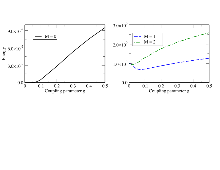
Figure 1: (Color online) Eigenvalues $E_{\rm FP}^{(M=0)}$ (left panel) and $E_{\rm FP}^{(M=1,2)}$ (right panel) of the Fokker–Planck Hamiltonian as a function of the coupling parameter $g$. Results have been computed by the diagonalization of the Fokker–Planck Hamiltonian (1) in the basis of the harmonic oscillator wavefunctions.

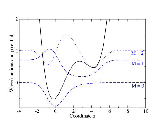
Figure 9: (Color online) The wavefunctions $\Phi^{(M)}_{\rm FP}(q)$ of the ground $M$ = 0 and the first excited $M$ = 1, 2 states of the Fokker–Planck Hamiltonian calculated at coupling parameter $g$ = 0.05. The base lines for the plots of the wave functions correspond to their energies $E_{\rm FP}^{(M)}(g)$.

Fokker–Planck energies of the lowest three eigenstates [of the potential (1)] found by matrix diagonalization are displayed in Fig. 1 as a function of the coupling $g$ (we use the notation $M=0,1,2$ in order to denote these three energy levels). As seen from this Figure, the states $M=1,2$ are degenerate in the limit $g\to 0$. A similar energy level splitting is well known for the symmetric double–well potential ZJJe2004i ; ZJJe2004ii ; JeZJ2001 and may be explained in terms of nonperturbative instanton contributions. In contrast to the double–well case, the Fokker–Planck potential contains a linear symmetry–breaking term [cf. Eq. (1)], and this term might be expected to lift any degeneracy. However, excited states can still develop a degeneracy for $g\to 0$ in view of the (only perturbatively broken) parity $\varepsilon\,=\,\pm 1$ of the quantum eigenstates. The ground state of the Fokker–Planck potential, however, is located in one of the wells and does not develop any degeneracy due to parity (see also Fig. 9 below).

It is interesting to investigate the adiabatic following of eigenvalues for the interpolating potential (7) as a function of the parameter $\eta$ for fixed $g$. This calculation (see Fig. 2) reveals that the identification of the double-well energy eigenvalues JeZJ2001 ; ZJJe2004i ; ZJJe2004ii with quantum numbers $(N,\varepsilon)$ for the double-well with the quantum number $M$ for the Fokker–Planck potential should proceed as follows:

$$(N=0,+)\Leftrightarrow \;M=0\,,$$ (8a)

$$(N=0,-)\Leftrightarrow \;M=1\,,$$ (8b)

$$(N=1,+)\Leftrightarrow \;M=2\,,$$ (8c)

$$(N=1,-)\Leftrightarrow \;M=3\,.$$ (8d)

The general relation is $M=2N+(1-\varepsilon)/2$. However, the asymptotic behavior of the eigenenergies for $g\to 0$ is different in the two cases:

$$E_{\rm dw}^{(N,\varepsilon)}(g)\to \;N+\frac{1}{2}\,,\qquad g\to 0\,,$$ (9a)

$$E_{\rm FP}^{(M)}(g)\to \;[\mkern-2.5mu[(M+1)/2]\mkern-2.5mu]\,,\qquad g\to 0\,,$$ (9b)

where $[\mkern-2.5mu[x]\mkern-2.5mu]$ is the integral part of $x$, i.e., the largest integer $m$ satisfying $m\leq x$. Equation (9b) implies that the perturbative contribution to the Fokker–Planck energy level with quantum number $M$ is given by Eq. (2) with $K=[\mkern-2.5mu[(M+1)/2]\mkern-2.5mu]$.

Apart from the degeneracy introduced by the instanton contributions, the eigenvalues $E^{(M=1,2)}_{\rm FP}(g)$ also have a qualitatively different dependence on $g$ when compared to the ground–state energy $E^{(M=0)}_{\rm FP}(g)$. As seen from Fig. 1, while the energy $E^{(M=0)}_{\rm FP}(g)$ increases monotonically as a function of the coupling constant $g$, the energies $E^{(M=1,2)}_{\rm FP}(g)$ have minima at $g_{0}\,\approx\,0.07$ and $g_{0}\,\approx\,0.025$, respectively.

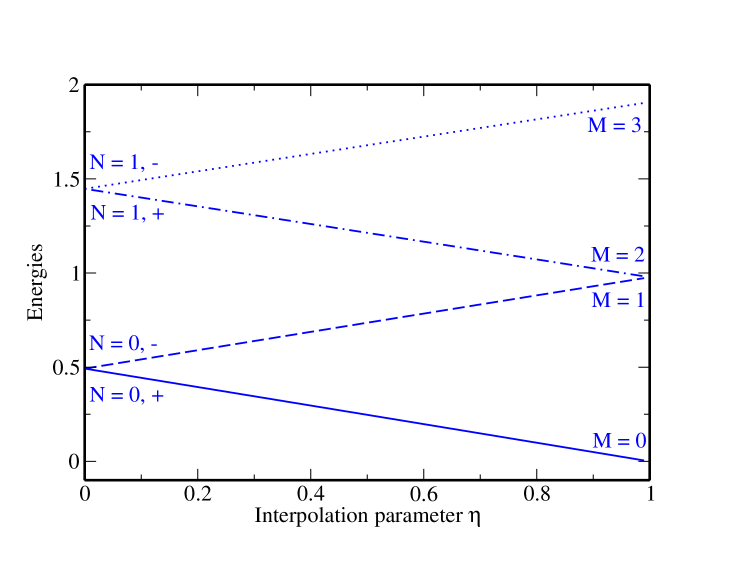
Figure 2: (Color online) Adiabatic following of the lowest four eigenvalues of the interpolating potential (7) from $\eta=0$ (double-well) to $\eta=1$ (Fokker–Planck potential). The value of the coupling parameter is held constant at $g=0.007$.

III Resummations, Energy Eigenvalues and Quantum Dynamics

III.1 Resummation of the resurgent expansion

The generalized Bohr–Sommerfeld quantization condition (3) together with the expansions (4)—(5) of the $A_{\rm FP}$ and $B_{\rm FP}$ functions uniquely determines the eigenvalues of the Fokker–Planck Hamiltonian. For the ground state, the energy eigenvalue can be found by systematic expansion of (3) in powers of the two small parameters $\exp(-1/3g)$ and $g$, whereas for excited states, the parameters are $\exp(-1/6g)$ and $g$. Thus, for the Fokker–Planck potential, the particular form of the expansion differs for the ground vs. excited states.

Explicitly, the ground-state energy ($M=0$) is given by the resurgent expansion JeZJ2004plb :

$$E^{(0)}_{\rm FP}(g)=\sum^{\infty}_{n=1}\left({{\rm e}^{-1/3g}\over 2\pi}\right)^{n}\,\sum^{n-1}_{k=0}\left\{\ln\left(-\frac{2}{g}\right)\right\}^{k}\,\sum^{\infty}_{l=0}f^{(0)}_{nkl}\,g^{l}\,,$$ (10)

where the index $n$ denotes the order of the “instanton contribution”: $n=1$ is a one-instanton, $n=2$ is a two-instanton, etc. (as noted below, the one-instanton configuration involves a back-tunneling of the particle to the lower well for the ground state and thus has twice the action of the characteristic one-instanton effect for excited states). Another subtle point which should be recalled here is that the leading one-instanton term involves a summation over all possible $n$–instanton configurations but neglects instanton interactions ZJJe2004i . As seen from Eq. (10), the evaluation of the ground state energy within such a (first–order) approximation, also referred as a “dilute instanton gas” approximation, requires the knowledge of the $f^{(0)}_{10l}$ coefficients. Since these coefficients are available for download JeHomeHD , we only recall the six leading ones JeZJ2004plb :

$$f^{(0)}_{100} = 1\,,\quad f^{(0)}_{101}=-\frac{5}{6}\,,\quad f^{(0)}_{102}=-\frac{155}{72}\,,$$

$$f^{(0)}_{103} = -\frac{17315}{1296}\,,\quad f^{(0)}_{104}=-\frac{3924815}{31104}\,,$$ (11)

$$f^{(0)}_{105} = -\frac{294332125}{186624}\,,\quad f^{(0)}_{106}=-\frac{163968231175}{6718464}\,.$$

By inserting these coefficients in Eq. (10), we are able to perform now the numerical check of the validity of the one-instanton expansion for the ground state at small coupling. In Table 1, for example, the energy $E^{(0)}_{\rm FP}(g)$ is displayed for coupling parameters in the range 0.005 $\leq g\leq$ 0.03 and is compared to the “true” eigenvalues as obtained from the diagonalization of the Fokker–Planck potential in the basis of harmonic oscillator wavefunctions. As seen from Table 1, the ground state energy is dominated by the one-instanton effect for relatively small values of the coupling parameter $g\leq$ 0.01. For stronger coupling, however, large discrepancies between the “true” energies and the results of resummation of Eq. (10) at $n$ = 1 are found indicating the importance of the higher–instanton terms which take into account the instanton interactions. The evaluation of the higher–order corrections ($n\geq$ 2) to the ground–state energy $E^{(0)}_{\rm FP}(g)$ is, however, a very difficult task since it requires a double resummation of the resurgent expansion, in powers of both $g$ and $\exp(-1/3g)$. In the present work such a double summation based on sequentially adding higher-order instanton terms will not be performed. Still, for the sake of completeness, we here indicate the leading two–instanton JeZJ2004plb and three–instanton coefficients for the Fokker–Planck ground state:

$$f^{(0)}_{210} = 2\,,\quad f^{(0)}_{200}=2\gamma\,,$$

$$f^{(0)}_{211} = -\frac{10}{3}\,,\quad f^{(0)}_{201}=-\frac{10}{3}\gamma-3\,,$$ (12)

$$f^{(0)}_{310} = 8\,\gamma\,,\quad f^{(0)}_{300}=6\gamma^{2}+\frac{\pi^{2}}{6}\,,$$

$$f^{(0)}_{311} = -\frac{80}{3}\gamma-6\,,\quad f^{(0)}_{301}=-15\gamma^{2}-12\gamma-17+\frac{5}{12}\pi^{2}\,,$$

where $\gamma=0.577216\dots$ is Euler’s constant.

Table 1: Ground–state energy of the Fokker–Plank Hamiltonian. Results have been computed by the diagonalization of the Hamiltonian in the basis of the harmonic oscillator wavefunctions (”true” energy) and by resummation of Eq. (10) within the one-instanton approximation ($n$ = 1). The numerical uncertainty of the entries in the right column is estimated on the basis of the apparent convergence of results under an appropriate increase of the number of $f^{(0)}_{10l}$ parameters, which corresponds to the number of terms in the perturbative expansion about the leading instanton. Numerical discrepancies between the left and right column are due to higher-order instanton contributions, as described in the text. We underline those decimal figures in the one-instanton results which are equal to the corresponding ones in the complete numerical solution.

$g$	$E^{(M=0)}_{\rm FP}$ (diagonalization)	$n=1$ term of Eq. (10)
0.005	1.766 107 332 563 $\times$ 10-30	1.766 107 332 563 $\times$ 10-30
0.010	5.267 473 259 637 $\times$ 10-16	5.267 473 259 637 $\times$ 10-16
0.015	3.508 587 565 372 $\times$ 10-11	3.508 587 564 030 $\times$ 10-11
0.020	9.033 155 571 641 $\times$ 10-09	9.033 154 730 920 $\times$ 10-09
0.025	2.519 767 018 258 $\times$ 10-07	2.519 760 770 755(1) $\times$ 10-07
0.030	2.313 302 179 961 $\times$ 10-06	2.313 251 574 075(2) $\times$ 10-06

As seen from Eq. (10), no splitting into levels with positive and negative parity arises for the ground state of the Fokker–Planck potential due to the linear symmetry–breaking term in Eq. (1). This term modifies the potential in such a way that the leading, one-instanton ($n$ = 1) shift of the ground state energy results from a back–tunneling (instanton–antiinstanton configuration) of the particle to the lower well JeZJ2004plb . For excited states, in contrast, the one-instanton configuration is a trajectory which starts in one well and ends in the other, restoring the broken symmetry. Therefore, any excited state ($M>$ 0) of the Fokker–Planck Hamiltonian can be characterized by its principal quantum number

$$K=[\mkern-2.5mu[(M+1)/2]\mkern-2.5mu]$$ (13)

and the parity

$$\varepsilon=2\left(2K-M-\frac{1}{2}\right)\,.$$ (14)

In fact, this classification is very similar to the double-well potential (6) except, of course, the particular case of the ground state. It follows naturally that the resurgent expansion for the excited states of the Fokker–Planck potential is very close to the analogous expansion for the double–well potential and reads JeZJ2004plb :

$$E^{(M>0)}_{\rm FP}(g)=E^{(K,\varepsilon)}_{\rm FP}(g)=\sum_{l=0}^{\infty}E_{K,l}\,g^{l}$$

$$+\sum^{\infty}_{n=1}\left[-\varepsilon\,\Xi_{K}(g)\right]^{n}\,\sum^{n-1}_{k=0}\left\{\ln\left(-\frac{2}{g}\right)\right\}^{k}\,\sum^{\infty}_{l=0}f^{(K)}_{nkl}\,g^{l}\,,$$ (15)

where $E_{K,l}$ are perturbative coefficients and $\Xi_{K}(g)$ is given by

$$\Xi_{K}(g)=\frac{2^{K-1/2}}{g^{K}\,\sqrt{\pi\,K!\,(K-1)!}}\,\rm{e}^{-1/6g}\,.$$ (16)

The power of $\Xi$ can again be associated with the order of the instanton ($K=1$: one-instanton, $K=2$ means two-instanton, etc.). One should note that two intricacies are associated to the precise meaning of the quantities that enter Eq. (III.1):

• In analogy to the double-well potential, the imaginary part which is generated by the resummation of the perturbation series about the leading instanton (the “discontinuity” of the distributional Borel sum in the terminology of Ref. CaGrMa1986, ) is compensated by an explicit imaginary part that stems from the two-instanton effect [from the factor $\ln(-2/g)$]. Related questions have been discussed at length in Refs. ZJJe2004i, ; ZJJe2004ii, .

• In contrast to the ground–state energy (10), the leading contribution to the energies $E^{(\varepsilon,K>0)}_{\rm FP}(g)$ for small coupling arises from the perturbation expansion (2) which is manifestly nonvanishing to all orders in $g$. However, since this perturbation expansion is independent of the parity $\varepsilon$, the energy splitting of the levels with the same principal quantum number $K$ is again dominated by the one-instanton contribution ($n=1$).

Similar to the ground state (10), we may compute such a contribution and, hence, a splitting of an arbitrary excited state $K$ by making use of the $f^{(K)}_{10l}$ coefficients, which for $K>0$ read ($l=0,1,2,3$):

$$f^{(K)}_{100}= 1\,,\qquad f^{(K)}_{101}=-\frac{17}{2}K^{2}-6K-\frac{5}{12}\,,$$ (17a)

$$f^{(K)}_{102}= \frac{289}{8}K^{4}-\frac{23}{2}K^{3}-\frac{1139}{24}K^{2}-\frac{45}{4}K-\frac{695}{288}\,,$$ (17b)

$$f^{(K)}_{103}= -\frac{4913}{48}K^{6}+\frac{629}{2}K^{5}+\frac{1637}{32}K^{4}$$

$$-\frac{1885}{3}K^{3}-\frac{155825}{576}K^{2}-\frac{3835}{24}K-\frac{68885}{10368}\,.$$ (17c)

Results for $K\leq 28$ are available for download JeHomeHD . In Table 2, for example, the splitting $E^{(\varepsilon=-1,K=1)}_{\rm FP}(g)-E^{(\varepsilon=+1,K=1)}_{\rm FP}(g)$ of the first two excited states $M=1,2$ due to the one-instanton effect ($n$ = 1) is displayed as a function of the coupling parameter $g$. Again, a comparison of the results obtained by the resummation of Eq. (III.1) and by the diagonalization of the Fokker–Planck Hamiltonian indicates the importance of the higher–instanton effects ($n>$ 1) and, hence, the necessity of a double resummation of the resurgent expansion, in powers of both $g$ and $\exp(-1/6g)$. Instead of performing such a double summation explicitly, it is more convenient to enter directly into the quantization condition (3), with resummed quantities as defined by the $A_{\rm FP}(E,g)$ and $B_{\rm FP}(E,g)$ functions. We discuss this alternative approach in the next Section.

Table 2: Energy difference between the excited states $E^{(M=1,2)}_{\rm FP}(g)$ of the Fokker–Planck Hamiltonian. Results have been computed by diagonalizing the Hamiltonian in the basis of the harmonic oscillator wavefunctions (left column) and by resummation of Eq. (III.1) within the one-instanton approximation (right column). The numerical uncertainty is estimated on the basis of the apparent convergence of results under an appropriate increase of the number of $f^{(K)}_{10l}$ parameters. As in Table 1, we underline those decimal figures in the one-instanton results which are equal to the corresponding ones in the complete numerical solution.

$g$	$E^{(M=2)}_{\rm FP}-E^{(M=1)}_{\rm FP}$ (diag.)	$n=1$ term of Eq. (III.1)
0.005	9.848 553 978 903 $\times$ 10-13	9.848 553 978 903 $\times$ 10-13
0.010	7.801 059 663 554 $\times$ 10-06	7.801 059 659 99(1) $\times$ 10-06
0.015	1.213 924 539 483 $\times$ 10-03	1.213 91 452(2) $\times$ 10-03
0.020	1.289 613 568 640 $\times$ 10-02	1.288 765(1) $\times$ 10-02
0.025	4.633 794 364 814 $\times$ 10-02	4.611 6(1) $\times$ 10-02
0.030	9.699 341 140 782 $\times$ 10-02	9.610 2(6) $\times$ 10-02

III.2 Resummation of the quantization condition

The resurgent expansions (10) and (III.1) for the energies of the ground and excited states of the Fokker–Planck Hamiltonian follow as a direct consequence of the quantization condition (3). As seen from our calculations summarized in Tables 1 and 2, these expansions are very useful for small coupling, but not of particular usefulness even for rather moderate values of $g$, because of the necessity of their double resummation. Here, we would like to investigate whether it is possible to resum the divergent series that gives rise to $A_{\rm FP}(E,g)$ and $B_{\rm FP}(E,g)$ directly and look for solutions of the quantization condition (3) without any intermediate recourse to the resurgent expansion. In fact, this approach currently appears to be the only feasible way to evaluate the multi–instanton expansion (in powers of $n$), because the quantization condition incorporates all instanton orders.

In order to introduce such a “direct summation” approach, we recall that the solution of the generalized Bohr–Sommerfeld quantization condition (3) for a particular coupling parameter $g$ must provide the energy spectrum of the Fokker–Planck Hamiltonian. In other words, if one defines the left–hand side of the quantization condition (3) as a function of two variables $E$ and $g$:

$$Q(E,g)= \,\frac{1}{\Gamma(-B_{\rm FP}(E,g))\,\Gamma(1-B_{\rm FP}(E,g))}$$

$$+\left(-\frac{2}{g}\right)^{2B_{\rm FP}(E,g)}\frac{{\rm e}^{-A_{\rm FP}(E,g)}}{2\pi}\,,$$ (18)

then the zeros of this function at fixed $g$ determine the energy spectrum of (1):

$$Q(E^{(M)}_{\rm FP}(g),g)\,=\,0,\qquad M=0,1,2,....\,.$$ (19)

A numerical analysis of the function $Q(E,g)$ can be used, therefore, in order to examine the validity and applicability of the generalized quantization condition given by Eqs. (3)—(5) for the case of strong coupling.

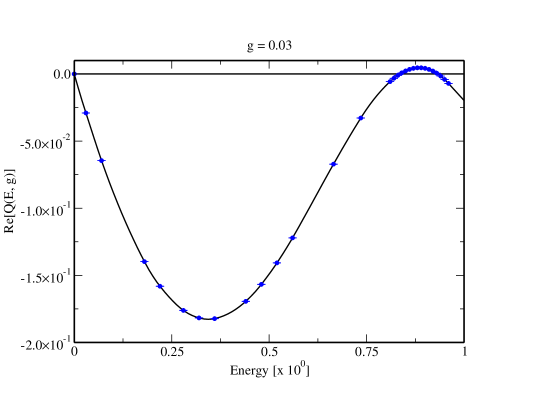
Figure 3: (Color online) Energy dependence of (the real part of) the function $Q(E,g)$. Calculations have been performed for fixed $g=0.03$.

As seen from Eq. (III.2), any analysis of the function $Q(E,g)$ can be traced back to the evaluation of the functions $A_{\rm FP}(E,g)$ and $B_{\rm FP}(E,g)$ which constitute series in two variables, namely $E$ and $g$ [cf. Eqs. (4)—(5)]. In order to compute these series, it is convenient to re–write the functions $A_{\rm FP}(E,g)\equiv A_{\rm FP}(E,gx)|_{x=1}$ and $B_{\rm FP}(E,g)\equiv B_{\rm FP}(E,gx)|_{x=1}$ as (formal) power series in terms of a variable $x$, taken at $x$ = 1 [cf. §8.5 of Ref. Ha1949, ]:

$$B_{\rm FP}(E,g)\,=\,\sum\limits_{n=0}^{N_{max}}\left.b^{(n)}_{\rm FP}(E,g)\,x^{n}\right|_{x=1}\,,$$ (20)

$$A_{\rm FP}(E,g)-\frac{1}{3g}\,=\,\sum\limits_{n=0}^{N_{max}}\left.a^{(n)}_{\rm FP}(E,g)\,x^{n}\right|_{x=1}\,,$$ (21)

where the coefficients $a^{(n)}_{\rm FP}(E,g)$ and $b^{(n)}_{\rm FP}(E,g)$ are uniquely determined by Eqs. (4) and (5): $b^{(0)}_{\rm FP}(E,g)\,=\,E$, $b^{(1)}_{\rm FP}(E,g)\,=\,3E^{2}g$, etc. In the computations, the power series (20) and (21) allow one to use a unified computer algebra routine for the Borel–like summations, which simply takes as input the variables $a^{(n)}_{\rm FP}(E,g)$ and $b^{(n)}_{\rm FP}(E,g)$, as a function of $g$ and returns the value of the resummed series at $x=1$. Indeed, this routine can be universally used for different values of $g$ and is therefore convenient for further numerical computations which are discussed below.

Making use of Eqs. (20) and (21), we may now perform a simultaneous summation of the perturbation series as well as of the perturbation series about each of the instantons and find the functions $B_{\rm FP}(E,g)$ and $A_{\rm FP}(E,g)$, correspondingly, where we use the same notation for a function and its Borel sum. There is a small subtlety because for positive $g$, the power series (20) and (21) are nonalternating and divergent and, hence, special resummation techniques are required to calculate the Borel sums. In our present calculations, for example, we apply a generalized Borel–Padé method Je2000prd ; JeSo2001 . The discussion of this method is beyond the scope of the present work, and the reader is referred to Refs. FrGrSi1985, ; Je2000prd, ; JeSo2001, for a more detailed discussion. Because of their nonalternating property, the perturbation series defining the functions $A_{\rm FP}(E,g)$ and $B_{\rm FP}(E,g)$ are Borel summable only in the distributional sense CaGrMa1986 . The evaluation of the Borel–Laplace integral thus requires an integration along a contour which is tilted with respect to the real axis (for details see Refs. FrGrSi1985, ; Je2001pra, ; JeSo2001, and the contours $C_{+1}$ and $C_{-1}$ in Ref. Je2000prd, ). The resummation of the divergent series (20) and (21) may be carried out along each of these contours, but it is important to characterize the perturbative and instanton contributions in the same way, i.e. to deform the contours for $B_{\rm FP}(E,g)$ and $A_{\rm FP}(E,g)$ either above or below the real axis, consistently. In the terminology of Ref. CaGrMa1986, , one should exclusively use either “upper sums” or “lower sums,” but mixed prescriptions are forbidden. From a historical perspective, it is interesting to remark that the possibility of deforming the Borel integration contour had already been anticipated in a remark near the end of Chap. 8 of the classic Ref. Ha1949, .

Table 3: Ground–state energy of the Fokker–Plank Hamiltonian. Results have been computed by the diagonalization of the Hamiltonian in the basis of the harmonic oscillator wavefunctions (left column) and by solving Eq. (19), as indicated in the right column.

$g$	$E^{(0)}_{\rm FP}$ (diagonalization)	Zero of ${\rm Re}[Q(E,g)]$
0.010	5.267 473 259 637 $\times$ 10-16	5.267 473 259 637 $\times$ 10-16
0.030	2.313 302 179 961 $\times$ 10-06	2.313 302 17(2) $\times$ 10-06
0.070	1.267 755 797 982 $\times$ 10-03	1.267 74(6) $\times$ 10-03
0.100	5.199 138 696 222 $\times$ 10-03	5.199 3(2) $\times$ 10-03
0.170	2.079 244 408 360 $\times$ 10-02	2.078(1) $\times$ 10-02
0.300	5.318 357 438 655 $\times$ 10-02	5.323(9) $\times$ 10-02

We are now in the position to analyze the properties of the function $Q(E,g)$ and, hence, to extract the energy spectrum of the Fokker–Planck Hamiltonian. As mentioned above, to perform such an analysis for any particular $g$ we have to (i) resum the (divergent) series for the functions $A_{\rm FP}(E,g)$ and $B_{\rm FP}(E,g)$ and (ii) insert the resulting generalized Borel sums into Eq. (III.2). We may then interpret the $Q(E,g)$ as a function of $E$ (at fixed $g$) and (iii) numerically determine the zeros of this function which correspond to the energy values $E^{(M)}_{\rm FP}$ of the Fokker–Plank Hamiltonian, according to Eq. (19). In Fig. 3, for instance, we display the energy dependence of the real part of the function $Q(E,g)$ taken at $g=0.03$. In the energy range $0<E<1$, this function has three zeros which obviously correspond to the ground $E^{(0)}_{\rm FP}$ and to the excited $E^{(1,2)}_{\rm FP}$ states. The ground-state energy $E^{(0)}_{\rm FP}$ determined in such a way is presented in Table 3 and compared to reference values obtained by the diagonalization of the Hamiltonian matrix in the basis of harmonic oscillator wavefunctions. Moreover, apart from the particular case of $g=0.03$, we also display the energy $E^{(0)}_{\rm FP}$ for other coupling parameters spanning the range from $g=0.01$ to $g=0.3$ (see also Fig. 4). This rather wide range of coupling parameters $g$ considered here allows us to investigate the behavior of the generalized Bohr–Sommerfeld quantization condition in the transition from weak to strong coupling. As seen from Table 3, the ground–state energy is well reproduced at $g=0.01$ (up to 14 decimal digits). Alternatively, a highly accurate value of the ground state energy (at $g=0.01$) can be obtained from the the one-instanton contribution to the resurgent expansion (10) for $g<0.01$, as indicated in Table 1. The accuracy of the one-instanton approximation is rapidly decreasing for higher $g$. For instance, at the moderate value of $g=0.03$, the one-instanton term of the resurgent expansion (10) reproduces the ground-state energy only to four decimal digits (see the last row of Table 1), while a total of eight digits can be obtained from solving Eq. (19), as indicated in the second row of Table 3. For even stronger coupling, one observes a much larger numerical uncertainty in the determination of the zeros of the function $Q(E,g)$, because the convergence of the generalized and optimized Borel–Padé methods employed in the resummation of the $A_{\rm FP}(E,g)$ and $B_{\rm FP}(E,g)$ functions is empirically observed to reach fundamental limits for larger values of the coupling, which cannot be overcome by the use of multiprecision arithmetic and might indicate a fundamental limitation for the convergence of the transforms and are not due to numerical cancellations. It might be interesting to explore these limits also from a mathematical point of view. Specifically, we have determined the numerical uncertainty of the $A_{\rm FP}(E,g)$ and $B_{\rm FP}(E,g)$ functions on the basis of the apparent convergence of the Borel–Padé approximants, integrated in the complex plane and accelerated according to Ref. JeSo2001, , using an optimal truncation of the order of the transforms. We found that as the order of the Borel–Padé transformation was increased, the apparent convergence of the transforms stopped at around order 40 for $g=0.03$ and higher. Despite these difficulties, the generalized Bohr–Sommerfeld quantization formula (19) determines the ground–state energy of the Fokker–Planck potential with an accuracy of about 0.01 % up to $g\leq 0.3$ (cf. Table 3).

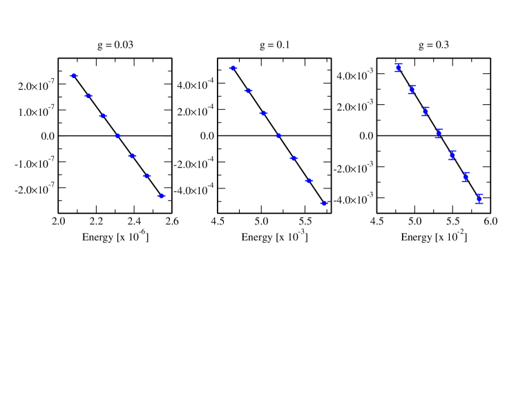
Figure 4: (Color online) Energy dependence of (the real part of) the function $Q(E,g)$. As in Fig. 3, the results of linear regression analysis of the function $Q(E,g)$ are depicted by the solid line. Calculations have been performed around the “true” energies of the ground state and for the different values of the coupling parameter: $g$ = 0.03 (left panel), $g=0.1$ (middle panel) and $g=0.3$ (right panel). The energy eigenvalues obtained using the displayed graphs determine the corresponding entries in the right column of Table 3.

Until now we have discussed the computation of the ground–state energy $E^{(0)}_{\rm FP}$ of the Fokker–Planck Hamiltonian. Of course, the function $Q(E,g)$ may also help to determine the energies of excited states. In contrast to the ground state, however, the numerical analysis of the function $Q(E,g)$ for excited states is more complicated due to bad convergence of the Borel sums for the $A_{\rm FP}(E,g)$ and $B_{\rm FP}(E,g)$ functions in the energy range relevant for the excited states. As seen from Fig. 5, the convergence problems lead to relatively large numerical uncertainties for the numerical calculation of the function $Q(E,g)$ already for a relatively mild coupling parameter $g=0.07$. We recall that this value of $g$ corresponds to the minimum of the energy $E_{\rm FP}^{(M=1)}(g)$ as a function of $g$ and thus can be naturally identified as marking the transition from weak to strong coupling. As a result of the numerical uncertainties, the energy $E_{\rm FP}^{(M=1)}(g=0.07)$ of the first excited state may be reproduced only up to 2 decimal digits (see Table 4). For even larger values of parameter $g$, the maximal accuracy of calculations, based on Eq. (19), is only a single significant digit, even though the double resummation of the instanton expansion, and of the perturbative expansion about each instanton, is implicitly contained in the cited Equation.

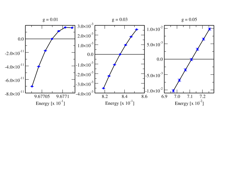
Figure 5: (Color online) Energy dependence of (the real part of) the function $Q(E,g)$. The results for the zeroes of $Q(E,g)$ obtained by a quadratic regression analysis are depicted by solid lines. Calculations have been performed around the ”true” energies of the first excited state with $K$ = 1, $\varepsilon$ = +1 ($M$ = 1) and for three different values of the coupling parameter: $g=0.01$ (left panel), $g=0.03$ (middle panel) and $g=0.05$ (right panel). The energy eigenvalues obtained using the displayed graphs determine the corresponding entries in the right column of Table 4.

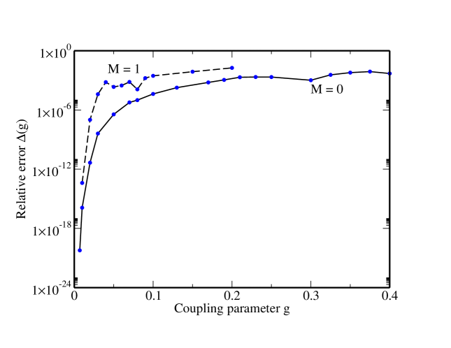
Figure 7: (Color online) Relative error (22) of calculations of the eigenvalues as a function of coupling constant $g$. Results are presented for the ground ($M$ = 0) and the first excited ($M$ = 1) states of the Fokker–Planck potential.

Supplementing the the specific Fokker–Planck energies of the $M=0,1$ states presented in Tables 3 and 4, we indicate in Fig. 6 the $g$–dependence of the energies $E^{(0)}_{\rm FP}$ and $E^{(1)}_{\rm FP}$ as obtained from the analysis of the function $Q(E,g)$ and compare to reference values obtained from the diagonalization of the Hamiltonian matrix. As indicated in Fig. 6, the results obtained by a direct resummation of the quantization condition give a good quantitative picture of the ground–state and the first excited–state eigenvalues in the ranges $0\leq g\leq 0.7$ and $0\leq g\leq 0.3$, respectively. The behavior of the numerical uncertainty as a function of $g$ is explicitly shown in Fig. 7, where we plot the quantity

$$\Delta(g)\,=\,\left|\frac{E_{\rm FP,\,resum}^{(M)}(g)-E_{\rm FP,\,diag}^{(M)}(g)}{E_{\rm FP,\,diag}^{(M)}(g)}\right|\,,$$ (22)

with $E^{(M)}_{\rm FP,\,resum}(g)$ and $E_{\rm FP,\,diag}^{(M)}(g)$ being the eigenvalues as obtained from the direct resummation of the quantization condition given in Eq. (19) and the diagonalization of the Hamiltonian (1), respectively (the latter values, which are numerically more accurate, are taken as the reference values). While the accuracy of resummations for the ground–state energy remains satisfactory even for (relatively) strong coupling, the relative error for the first excited is numerically much more significant.

Table 4: The energy of the first excited state with $M=1$ of the Fokker–Planck Hamiltonian. Results have been computed by the diagonalization of the Hamiltonian in the basis of the harmonic oscillator wavefunctions (exact energy) and by solving Eq. (19).

$g$	$E^{(M=1)}_{\rm FP}$ (diagonalization)	zero of the Re[$Q(E,g)$]
0.010	9.677 074 461 352 $\times$ 10-01	9.677 074 461 352 $\times$ 10-01
0.020	9.219 489 780 495 $\times$ 10-01	9.219 490(3) $\times$ 10-01
0.030	8.354 795 860 905 $\times$ 10-01	8.354 4(6) $\times$ 10-01
0.070	6.828 548 309 058 $\times$ 10-01	6.833(4) $\times$ 10-01
0.200	8.710 869 037 634 $\times$ 10-01	8.76(5) $\times$ 10-01
0.250	9.508 936 793 119 $\times$ 10-01	9.4(2) $\times$ 10-01

III.3 Strong–coupling expansion

As discussed in the previous Section, a numerical procedure based on the generalized Bohr–Sommerfeld formulae may provide relatively accurate estimates of the ground as well as the (first two) excited–state energies for the coupling parameters in the range $0\leq g\leq 0.3$. The question arises whether $g\approx 0.3$ can be considered as belonging to the strong coupling regime. Since the minima of the first two excited-state energies occur at $g=0.07$ and $g=0.025$, respectively, one might be tempted to answer the question affirmatively. However, one could devise a different criterion for the transition to the strong coupling regime. For instance, one might define the strong–coupling region as a region of an appropriately specified large-coupling asymptotic behavior of the eigenvalues $E_{\rm FP}^{(M)}(g)$.

The large–coupling asymptotics of the Fokker–Planck potential thus represents a natural next aim in the current investigation. To this end, we apply a so–called Symanzik scaling $q\rightarrow g^{-1/6}q$ in Eq. (1) and rewrite the Fokker–Planck potential into another one with the same eigenvalues but a fundamentally different structure SiDi1970 ; We1996b :

$$H_{\rm FP}=g^{1/3}\left[H_{\rm L}+\left(-q^{3}-\frac{1}{2}\right)g^{-1/3}+\frac{q^{2}}{2}g^{-2/3}\right]\,,$$ (23)

where the Hamiltonian $H_{\rm L}$ does not depend on $g$:

$$H_{\rm L}=-\frac{1}{2}\left(\frac{d}{dq}\right)^{2}+q+\frac{q^{4}}{2}\,.$$ (24)

We conclude that the $M$th eigenvalue of the Fokker–Planck Hamiltonian for the $g\rightarrow\infty$ is determined in leading order by the $M$th eigenvalue $E_{\rm L}^{(M)}$ of the Hamiltonian (24):

$$E_{\rm FP}^{(M)}(g)\approx g^{1/3}E_{\rm L}^{(M)}\,.$$ (25)

Moreover, Eq. (25) also indicates that the classifications of the levels $M=0,1,2,\dots$ of the Fokker–Planck and the $H_{\rm L}$ Hamiltonians are obviously identical in the strong–coupling regime.

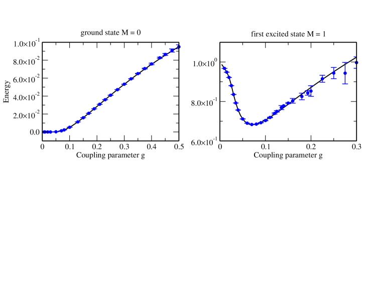
Figure 6: (Color online) Eigenvalues $E^{(M=0)}_{\rm FP}$ (left panel) and $E^{(M=1)}_{\rm FP}\equiv E^{(K=1,\varepsilon=+1)}_{\rm FP}$ (right panel) of the Fokker–Planck Hamiltonian as a functions of the coupling parameter $g$. Results have been computed by the diagonalization of the Fokker–Planck Hamiltonian in the basis of the harmonic oscillator wavefunctions (solid lines) and by solving Eq. (19), where the latter correspond the the data points with the error bars.

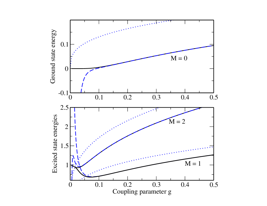
Figure 8: (Color online) Exact values (solid line) for the ground state and the two lowest excited energy levels for the Fokker–Planck potential as a function of $g$, together with the leading asymptotics (dotted line) and the partial sum of the strong-coupling expansion (dashed line) as defined by the first six nonvanishing terms in powers of $g^{-2k/3}$ [see Eq. (26)], which are listed in Table 3. Note that the leading strong-coupling asymptotics alone cannot satisfactorily describe the true energy eigenvalues for moderate and small coupling. By contrast, the partial sum of the first six nonvanishing terms of the strong-coupling asymptotics yields numerical values which are indistinguishable from the true eigenvalues on the level of the line thickness used in the plots, down to rather small values of the coupling (dashed vs. solid lines).

Based on Eq. (25), we now wish to compute the leading asymptotics of the ground $E_{\rm FP}^{(M=0)}(g)$ and excited–state $E_{\rm FP}^{(M=1,2)}(g)$ energies of the Fokker–Planck Hamiltonian. This computation obviously requires information about the corresponding eigenvalues of the Hamiltonian $H_{\rm L}$. The energies $E_{\rm L}^{(M)}$ have again been determined by a diagonalization of the Hamiltonian matrix within a basis of up to 1000 harmonic oscillator wavefunctions and than utilized in Eq. (25). As seen from Fig. 8, the leading asymptotics of the eigenvalues $E_{\rm FP}^{(M=0,1,2)}(g)$ (dotted line), calculated in such a way, significantly overestimate the energies of the Fokker–Planck Hamiltonian for the region $0\leq g\leq 0.3$. Higher–order corrections to the large-coupling asymptotics are therefore required, in order to reproduce more accurately the asymptotics of the eigenvalues $E_{\rm FP}^{(M=0,1,2)}(g)$. We observe that we may apply standard Rayleigh–Schrödinger perturbation theory to Eq. (23) and use the fact that the perturbative with respect to $H_{\rm L}$, which is $V(g)=\left(-q^{3}-1/2\right)g^{-1/3}+q^{2}g^{-2/3}/2$, remains Kato–bounded with respect to the unperturbed Hamiltonian $H_{\rm L}$ for large $g$. Within such an approach, a strong–coupling perturbation expansion can be written for each energy $E_{\rm FP}^{(M)}(g)$:

$$E_{\rm FP}^{(M)}(g)=g^{1/3}\sum\limits_{k=0}^{\infty}L^{(M)}_{k}g^{-2k/3}\,$$ (26)

where $L^{(M)}_{0}\equiv E_{\rm L}^{(M)}$ and the higher perturbation coefficients $L^{(M)}_{k>0}$ are calculated in the basis of the wavefunctions of the unperturbed Hamiltonian (24). The first six $L^{(M)}_{k}$ coefficients for the ground $M$ = 0 as well as the first excited $M$ = 1, 2 states are given in Table 5.

In Fig. 8, we implemented the first few expansion coefficients as listed in Table 5, in order to calculate strong-coupling asymptotics for the three lowest levels of the Fokker–Planck Hamiltonian (dashed lines). Obviously, the partial sum of the expansion (26) as defined by only six coefficients provides much better agreement with numerically determined energy eigenvalues than the leading asymptotics (25). For instance, the energy of the first excited state $M=1$ is very well described by the (first six terms of the) strong–coupling expansion already at $g=0.07$ (the agreement is better than one percent). This point, which also corresponds to the minimum of the function $E_{\rm FP}^{(M=1)}(g)$, can thus naturally be identified as the transition region between the regimes of weak and strong coupling. By using such a definition for the transitory regime, we may finally conclude that the resummation of the Bohr–Sommerfeld quantization formulae (3)–(5), using the condition (19), may provide reasonable estimates for the energy levels $E_{\rm FP}^{(M)}(g)$ even in a limited subregion of the strong-coupling regime.

III.4 Quantum dynamics

In previous Sections of the current paper, we have presented a systematic study of the energy spectrum of the Fokker–Planck potential. In particular, two methods for computing the eigenvalues $E_{\rm FP}^{(M)}(g)$ have been discussed in detail: (i) a “brute–force” method which is based on the diagonalization of the Hamiltonian matrix and (ii) a generalized perturbative approach which accounts for the instanton effects. While, of course, the precise computation of the energy levels is a very important task, the complete description of the properties of the particular Hamiltonian also requires an access to its wavefunctions $\Phi^{(M)}_{\rm FP}(q)$. Most naturally, these wavefunctions may be obtained together with the eigenvalues $E_{\rm FP}^{(M)}(g)$ by matrix diagonalization. In our calculations, the basis of the standard harmonic oscillator wavefunction $\{\phi_{n}(q)\}_{n=0}^{\infty}$ is used for the construction of a Hamiltonian matrix $\left\langle\phi_{n}\left|H_{\rm FP}\right|\phi_{m}\right\rangle$. The Fokker–Planck eigenfunctions are thus given by:

$$\Phi^{(M)}_{\rm FP}(q)=\sum\limits_{n=0}^{\infty}c^{(M)}_{n}\phi_{n}(q)\,,$$ (27)

where the coefficients $c^{(M)}_{n}$ are found by the diagonalization procedure. In Fig. 9 we display, for example, the wavefunctions (27) of the ground $M$ = 0 and the first excited $M=1,2$ states as calculated for a coupling parameter $g=0.05$. As is evident from Fig. 9, the symmetry–breaking term of the Hamiltonian (1) leads to a ground–state wavefunction $\Phi^{(M=0)}_{\rm FP}(q)$ (dashed line) which is neither a symmetric nor antisymmetric combination of the wavefunctions of the right and left wells, but localized in the lower well. For the first excited states, in contrast, the symmetry is partially restored, and we may attribute the wavefunctions $\Phi^{(M=1)}_{\rm FP}(q)$ (dashed and dotted line) and $\Phi^{(M=2)}_{\rm FP}(q)$ (dotted line) to states with positive ($\varepsilon$ = +1) and negative ($\varepsilon$ = -1) parities [see also Eqs. (13)—(14)].

Table 5: $L^{(M)}_{k}$ coefficients of the strong–coupling perturbation expansion (26) of the eigenvalues $E_{\rm FP}^{(M=0,1,2)}$ of the Fokker–Planck Hamiltonian.

$j$	$M=0$	$M=1$	$M=2$
0	$0.281\,067\,805$	$1.854\,587\,292$	$3.686\,419\,624$
1	$-0.132\,985\,313$	$-0.209\,853\,650$	$-0.307\,985\,031$
2	$0.021\,367\,333$	$0.028\,174\,214$	$0.025\,765\,237$
3	$-0.000\,876\,935$	$0.000\,220\,875$	$-0.000\,099\,791$
4	$-0.000\,060\,335$	$0.000\,031\,789$	$-0.000\,002\,135$
5	$-0.000\,001\,557$	$0.000\,000\,739$	$-0.000\,000\,385$

Until now, we have only discussed the evaluation of the eigenstates and eigenenergies of the Fokker–Planck Hamiltonian. In theoretical studies of double quantum-dot nanostructures GrDiJuHa1991 ; Op1999 ; GrHa1998 ; TsOp2004 and of the quantum tunneling phenomena in atomic physics LiBa1990 ; LiBa1992 , a large number of problems arise, in which the time-propagation of some (specially prepared) wavepacket in double-well-like potentials has to be considered. The methods for such a time-propagation, such as the well-known Crank-Nicolson method, the split-operator technique, and approaches based on the Floquet formalism and many others, are discussed in detail in the literature (see, e.g., Refs. GrDiJuHa1991, ; GrHa1998, ; CrNi1947, ; FlMoFe1976, ; PrKeKn1997, ). As a supplement to our previous considerations, we will now consider the time-propagation of an initial wavepacket in a double-well-like potential, recalling the adiabatic approach as one of the most simple and best-known techniques (see, e.g., the book Te2003, and references therein) for the integration of the (time–dependent) single particle Schrödinger equation. Within such a technique, in which we can naturally make use of the results previously derived for the eigenstates and eigenenergies, the propagation of a wavepacket $\Psi(q,t)$ in the (time–independent) Fokker–Planck potential (1) is given by:

$$\Psi(q,t)=\sum\limits_{M=0}^{\infty}b^{(M)}\,\exp\left(-{\rm i}\,E^{(M)}_{\rm FP}t\right)\,\Phi^{(M)}_{\rm FP}(q)\,.$$ (28)

Here the coefficients $b^{(M)}=\left\langle\Phi^{(M)}_{\rm FP}\left|\right.\Psi(t=0)\right\rangle$ determine the decomposition of the initial wavepacket (at $t$ = 0) in the basis of the eigenfunctions (27).

Equation (28) provides an exact solution for the wavefunction $\Psi(q,t)$ at an arbitrary moment of time only in the limit of an infinitely large basis of harmonic oscillator $\{\phi_{n}(q)\}_{n=0}^{\infty}$ and Fokker–Planck $\{\Phi^{(M)}_{\rm FP}(q)\}_{M=0}^{\infty}$ wavefunctions. For computational reasons, however, summations over basis functions have to be restricted to a finite number. In our calculations, basis sets of 300–1000 wavefunctions have been applied depending on the parameters of the initial wavepacket and the coupling parameter $g$. The actual size of the basis has been chosen according to the numerical checks of the Ehrenfest theorem or the normalization of the wavepacket.

Within the adiabatic approximation, which is valid for slowly varying potentials Te2003 ; CN , we may divide the time evolution of the potential into small intervals $\Delta t$ and assume that for every $k$th interval the Hamiltonian is time–independent and the propagation of the wavepacket is governed again by Eq. (28) where, of course, eigenvalues $E^{(M)}_{\rm FP}$ and eigenfunctions $\Phi^{(M)}_{\rm FP}(q)$ should be replaced with the eigenvalues $E^{(M)}_{k}$ and eigenfunctions $\Phi^{(M)}_{k}(q)$ of the Hamiltonian $H_{k}\equiv H(t_{k})$. We have applied this adiabatic time–propagation method, whose variations are well known from the literature HwPe1977 ; Ve2000 ; Su2003 ; Te2003 and which is equivalent to an exponentiation of the instantaneous Hamiltonian for each time interval $\Delta t$, to investigate the evolution of an (initially) Gaussian wavepacket in a time–dependent potential (7) which oscillates sinusoidally between the Fokker–Planck and the double-well cases. Since the animated results of this simulation are available for downloadJeHomeHD , we just present a small series of snapshots in Fig. 10. As seen from these pictures, the wavepacket, which is initially located in the right well, performs oscillations between the wells. These oscillations are controlled by the temporal change of the potential (7). We have checked empirically that the adiabatic approximation employed here does not represent an obstacle for an accurate time evolution in even rapidly oscillating potentials, because of the calculational efficiency of the other steps in our time propagation algorithm (notably, the diagonalization including the determination of eigenvectors can be implemented in a computationally very favorable way on modern computers). It is thus possible to perform quantum dynamical simulations in potentials which oscillate between two limiting forms with two fundamentally different characteristic ground-state configurations, each of which is governed by instantons, though in a different way. A generalization of our approach to two-dimensional potentials appears to be feasible and is currently being studied.

IV Conclusions

In this paper, we have investigated the Fokker–Planck [Eq. (1)] and the double-well [Eq. (6)] potential from the point of view of large-order perturbation theory (resurgent expansion and generalized quantization condition), in order to map out the regimes of validity of the instanton-related resurgent expansion for the lowest energy levels, and in order to explore the possibility of reaching the strong-coupling regime via a direct resummation of the $A_{\rm FP}$ and $B_{\rm FP}$ functions given in Eqs. (4) and (5), which enter the generalized quantization condition (3). The latter approach entails a complete double resummation of the resurgent expansions (10) and (III.1) both in powers of the instanton coupling $\exp(-1/6g)$ and in powers of the coupling $g$ (perturbative expansion about each instanton). The quest has been to explore the applicability of resummed expansions for medium and large coupling parameters, in the transitory regime to large coupling.

It is quite natural to identify the transition region for the first excited state as defined by the minimum of the energy level $E_{\rm FP}^{(M=1)}(g)$ as a function of $g$ (see the right panel of Fig. 6), which occurs near $g\approx 0.07$. As is evident from Figs. 6 and 8, it is possible to reach convergence for both the resummed secular equation (19) as well as convergence of the strong-coupling expansion (26) in a somewhat restricted overlap region $0.04\lesssim g\lesssim 0.3$. The question whether it is possible to use the resummed instanton expansion for large coupling, cannot universally be answered affirmatively, although it is reassuring to find at least a restricted region of overlap. In order to interpret the overlap, one should remember that for typical Borel summable series as they originate in various contexts in field theory, it is much easier to perform resummations at moderate and even large coupling parameters than for the instanton-related case considered here. An example is the 30-loop resummation of the anomalous dimension $\gamma$ function of six-dimensional $\phi^{3}$-theories and of Yukawa model theories BrKr2000 , which lead to excellent convergence for couplings as large as $g=10$ and higher JeSo2001 .

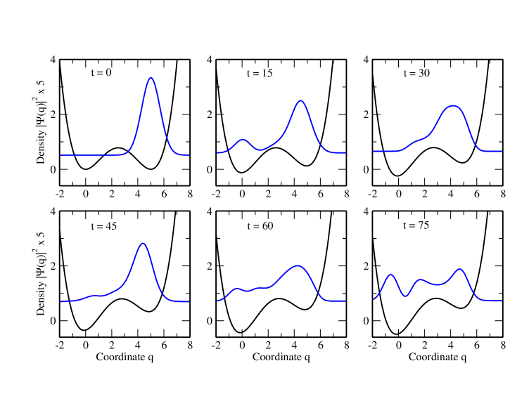
Figure 10: (Color online) Time propagation of the (initially) Gaussian wavepacket in the time–dependent potential (7) with $\eta=\sin(t/60)$ which oscillates between the double–well and Fokker–Planck potentials. The base line for the plot of the wave function corresponds to its instantaneous energy.

For the latter case, it is even possible to obtain, numerically, the strong-coupling asymptotics on the basis of a resummed weak-coupling perturbation theory (see, e.g., Ref. Su2001, for a remarkable realization of this idea in an extremely nontrivial context). The general notion is that any perturbation (a potential in the case of quantum mechanics and an interaction Lagrangian in the case of field theory) determines the large-order behavior of perturbation series describing a specific physical quantity. However, the potential or interaction Lagrangian also determine the large-coupling expansion for the physical quantity under investigation. This means that there is a connection between the large-coupling expansion and the large-order behavior of the perturbation series generated in each theory, and this correspondence can be exploited in order to infer strong-coupling asymptotics even in cases where only a few perturbative terms are known Su2001 . According to our numerical results, the corresponding calculation of strong-coupling asymptotics on the basis of only a few perturbative terms would be much more difficult in cases where instantons are present, even if like in our case, additional information is present in the form of the generalized quantization condition (3).

We deliberately refrain from speculating about further implications of this observation and continue with a summary of the application-oriented results gained in the current investigation. Potentials of the double-well type are important for a number of application–oriented calculations, including Josephson junction qubits BeEtAl2003 ; WeEtAl2005 , inversion doubling in molecular physics Hu1927 ; Xu2005 , semiconductor double quantum dots LoDV1998 ; HoEtAl2002 ; HuEtAl2005 , as well as, in a wider context, Bose–Einstein condensates in multi–well traps StCeMo2004 ; AlStCe2005 ; StAlCe2006 ; AlEtAl2005 . For the latter case, a number of theoretical works have been performed recently in order to explore the time propagation of (one particle) wavepackets in driven double–well potentials GrDiJuHa1991 ; Op1999 ; TsOp2004 . In Sec. II.2 we discuss a numerical procedure for an accurate description of energy levels and of the corresponding wave functions, which can thus be used in order to construct basis sets for an accurate quantum dynamical time evolution of wave packets in both static as well as time–dependent potentials. This well-known adiabatic technique for the integration of the (single particle) time-dependent Schrödinger equation is briefly recalled in Sec. III.4. We illustrate this technique by a calculation for a potential which oscillates between the Fokker–Planck and the double-well cases, governed by a time-dependent interpolating parameter $\eta=\cos(\omega t)$ as given in Eq. (7). Similar calculations can be done for cases where the potential admits resonances as in the case of a cubic anharmonic oscillator. In this case, the method of complex scaling leads to a basis of states which can be used in order to start quantum dynamical simulations. Related work is currently in progress.

V Acknowledgments

U.D.J. acknowledges support from the Deutsche Forschungsgemeinschaft (Heisenberg program). M.L. is grateful to Max–Planck–Institute for Nuclear Physics for the stimulating atmosphere during a guest researcher appointment, on the occasion of which the current work was completed.

Appendix A Supersymmetry and the Fokker–Planck Potential

This appendix is meant to provide a brief identification of the Fokker–Planck potential (1) in terms of a supersymmetric (SUSY) algebra CoKhSu1995 ; KaSo1997 . We define the operators

$$B^{\pm}=\frac{1}{\sqrt{2}}\,\left(W(q)\mp\frac{d}{dq}\right)$$ (29)

with $W(q)=q\,(1-\sqrt{g}\,q)$ and the SUSY Hamiltonian

$$H_{\rm SUSY}=\left(\begin{array}[]{cc}B^{+}B^{-}&0\\ 0&B^{-}B^{+}\end{array}\right)=\left(\begin{array}[]{cc}H_{1}&0\\ 0&H_{2}\end{array}\right)\,.$$ (30)

with

$$H_{1}= -\frac{1}{2}\left(\frac{d}{dq}\right)^{2}+\frac{1}{2}q^{2}\left(1-\sqrt{g}q\right)^{2}+\sqrt{g}q-\frac{1}{2}\,,$$ (31a)

$$H_{2}= -\frac{1}{2}\left(\frac{d}{dq}\right)^{2}+\frac{1}{2}q^{2}\left(1-\sqrt{g}q\right)^{2}-\sqrt{g}q+\frac{1}{2}\,.$$ (31b)

Notice that $W(q)$ finds a natural interpretation as a “superpotential” in the sense of Refs. CoKhSu1995, ; KaSo1997, . The Hamiltonians $H_{1}$ and $H_{2}$ are “superpartners.” They are related to each other by a simple reflection and translation, $q\to 1/\sqrt{g}-q$, and have the same spectra. In that sense, one may say that the Fokker–Planck potential is its own superpartner. The Fokker–Planck potential therefore constitutes a case of “broken supersymmetry” with zero Witten index [see, e.g., Eq. (2.88) of Ref. KaSo1997, ]. The construction of the supersymmetric partner thus does not help in the analysis of the Fokker–Planck Hamiltonian. One is forced into the instanton-inspired analysis presented in the current study.

As a last remark, we recall that the Fokker–Planck potential

$$V_{\rm FP}(q)=\frac{1}{2}q^{2}\left(1-\sqrt{g}q\right)^{2}+\sqrt{g}q-\frac{1}{2}=\frac{1}{2}\,\left[W^{2}(q)-W^{\prime}(q)\right]$$ (32)

could be assumed to admit a zero eigenvalue. However, as is evident from the discussion following Eq. (7.28) of Ref. ZJJe2004ii, , the corresponding eigenfunction is not normalizable, and thus cannot be interpreted as a physical state vector. Neither the Fokker–Planck potential nor its isospectral supersymmetric partner admit a zero eigenvalue.

References

- (1) J. Zinn-Justin and U. D. Jentschura, Ann. Phys. (N.Y.) 313, 197 (2004).
- (2) J. Zinn-Justin and U. D. Jentschura, Ann. Phys. (N.Y.) 313, 269 (2004).
- (3) U. D. Jentschura and J. Zinn-Justin, J. Phys. A 34, L253 (2001).
- (4) U. D. Jentschura and J. Zinn-Justin, Phys. Lett. B 596, 138 (2004).
- (5) I. W. Herbst and B. Simon, Phys. Rev. Lett. 41, 67 (1978).
- (6) M. Luban, J. H. Luscombe, M. A. Reed, and D. L. Pursey, Appl. Phys. Lett. 54, 1997 (1989).
- (7) D. Loss and D. P. DiVincenzo, Phys. Rev. A 57, 120 (1998).
- (8) A. W. Holleitner, R. H. Blick, A. K. Hüttel, K. Eberl, and J. P. Kotthaus, Science 297, 70 (2002).
- (9) A. K. Hüttel, S. Ludwig, H. Lorenz, K. Eberl, and J. P. Kotthaus, Phys. Rev. B 72, R081310 (2005).
- (10) F. Grossmann, T. Dittrich, P. Jung, and P. Hänggi, Phys. Rev. Lett. 67, 516 (1991).
- (11) L. A. Openov, Phys. Rev. B 60, 8798 (1999).
- (12) See the URL http://www.mpi-hd.mpg.de/~ulj.
- (13) J. Zinn-Justin, J. Math. Phys. 25, 549 (1984).
- (14) E. Caliceti, V. Grecchi, and M. Maioli, Commun. Math. Phys. 104, 163 (1986).
- (15) G. H. Hardy, Divergent Series (Clarendon Press, Oxford, UK, 1949).
- (16) U. D. Jentschura, Phys. Rev. D 62, 076001 (2000).
- (17) U. D. Jentschura and G. Soff, J. Phys. A 34, 1451 (2001).
- (18) V. Franceschini, V. Grecchi, and H. J. Silverstone, Phys. Rev. A 32, 1338 (1985).
- (19) U. D. Jentschura, Phys. Rev. A 64, 013403 (2001).
- (20) B. Simon and A. Dicke, Ann. Phys. (N.Y.) 58, 76 (1970).
- (21) E. J. Weniger, Ann. Phys. (N.Y.) 246, 133 (1996).
- (22) M. Grifoni and P. Hänggi, Phys. Rep. 304, 229 (1998).
- (23) A. V. Tsukanov and L. A. Openov, Semiconductors 38, 91 (2004).
- (24) W. A. Lin and L. E. Ballentine, Phys. Rev. Lett. 65, 2927 (1990).
- (25) W. A. Lin and L. E. Ballentine, Phys. Rev. A 45, 3637 (1992).
- (26) J. Crank and P. Nicolson, Proc. Camb. Phil. Soc. 43, 50 (1947).
- (27) J. A. Fleck, J. R. Morris, and M. D. Feit, Appl. Phys. A 10, 129 (1992).
- (28) M. Protopapas, C. H. Keitel, and P. L. Knight, Rep. Prog. Phys. 60, 389 (1997).
- (29) S. Teufel, Adiabatic Perturbation Theory in Quantum Dynamics — Lecture Notes in Mathematica Vol. 1821 (Springer, Berlin, Heidelberg, New York, 2003).
- (30) We note that our adiabatic approach, for slowly varying potentials, is limited essentially by the incompleteness of the basis used in each time propagation step, while the principal restriction of the familiar Crank–Nicolson time propagation algorithm (see Ref. CrNi1947 ) lies in the truncation of the exponential of the instantaneous Hamiltonian. Of course, for the one-dimensional problems studied here, an implementation of the Crank–Nicolson scheme also leads to a feasible alternative approach to the investigation of the quantum dynamics. In any case, the continuous monitoring of the Ehrenfest theorem and of the conservation of the normalization of the wavefunction provide important cross-checks for the computational consistency of the time propagation.
- (31) J. T. Hwang and P. Pechukas, J. Comp. Phys. 67, 4640 (1977).
- (32) E. P. Velicheva, Phys. At. Nucl. 63, 661 (2000).
- (33) A. A. Suzko, Phys. Lett. A 308, 267 (2003).
- (34) D. Broadhurst and D. Kreimer, Phys. Lett. B 475, 63 (2000).
- (35) I. M. Suslov, Pis’ma v. Zh. Éksp. Teor. Fiz. 74, 211 (2001), [JETP 74, 191 (2001)].
- (36) A. J. Berkley, H. Xu, R. C. Ramos, M. A. Gubrud, F. W. Strauch, P. R. Johnson, J. R. Anderson, A. J. Dragt, C. J. Lobb, and F. C. Wellstood, Science 300, 1548 (2003).
- (37) L. F. Wei, Y. X. Liu, and F. Nori, Phys. Rev. B 71, 134506 (2005).
- (38) F. Hund, Z. Phys. 43, 803 (1927).
- (39) C. N. Xuan, Chem. Phys. Lett. 406, 415 (2005).
- (40) A. I. Streltsov, L. S. Cederbaum, and N. Moiseyev, Phys. Rev. A 70, 053607 (2004).
- (41) O. E. Alon, A. I. Streltsov, and L. S. Cederbaum, Phys. Lett. A 347, 88 (2005).
- (42) A. I. Streltsov, O. E. Alon, and L. S. Cederbaum, Phys. Rev. A 73, 063626 (2006).
- (43) M. Albiez, R. Gati, J. Fölling, S. Hunsmann, M. Cristiani, and M. K. Oberthaler, Phys. Rev. Lett. 95, 010402 (2005).
- (44) F. Cooper, A. Khare, and U. Sukhatme, Phys. Rep. 251, 267 (1995).
- (45) H. Kalka and G. Soff, Supersymmetrie (B. G. Teubner, Stuttgart, 1997).