Nonlinear screening of charge impurities in graphene

Abstract

It is shown that a “vacuum polarization” induced by Coulomb potential in graphene leads to a strong suppression of electric charges even for undoped case (no charge carriers). A standard linear response theory is therefore not applicable to describe the screening of charge impurities in graphene. In particular, it overestimates essentially the contributions of charge impurities into the resistivity of graphene.

Graphene is a name given to an atomic layer of carbon atoms packed into a hexagonal two-dimensional lattice. This term is widely used to describe the crystal structure and properties of graphite (which consists from graphene layers relatively loosely stacked on top of each other), carbon nanutubes, and large fullerenes. Very recently, a way has been found to prepare free-standing graphenekostya0 ; kostya1 , that is, real two-dimensional crystal (in contrast with numerous quasi-two-dimensional systems known before). The graphene turns out to be a gapless semiconductor with a very high electron mobility which makes it a perspective material, e.g., for ballistic field-effect transistorkostya1 . It has been shownkostya2 ; kim that the charge carriers in graphene are massless Dirac fermions with effective “velocity of light” of order of 10⁶ ms^-1. Due to this unusual electronic structure graphene demonstrates exotic transport properties, such as a new kind of the integer quantum Hall effect with half-integer quantization of the Hall conductivitykostya2 ; kim ; gus ; per ; cas ; lee , or finite conductivity in the limit of zero charge-carrier concentration kostya2 ; ktsn ; been ; zieg .

One of peculiar transport properties of graphene, a mobility which is almost independent on the charge carrier concentrationkostya2 , was explained in Refs.nomura, ; ando, as a result of electron scattering by charge impurities. However, a linear-response theory was used to take into account screening effects. Rigorously speaking, this theory can be applied only assuming that the impurity potential is small in comparison with the Fermi energy; however, even in semiconductors where this condition can be, in general, broken this theory can be normally used and gives reasonable results (for the case of two-dimensional electron gas, see for review Ref.rmp, ).

In this paper we calculate nonlinear screening of charge impurities in graphene taking into account a “vacuum polarization” effect in a region of strong potential.

A general nonlinear theory of screening in the system of interacting particles can be formulated in a framework of the density functional approachkohn . In this theory a total potential $V\left(\mathbf{r}\right)$ acting on electrons equals

$$V\left(\mathbf{r}\right)=V_{0}\left(\mathbf{r}\right)+V_{ind}\left(\mathbf{r}\right)$$ (1)

where $V_{0}\left(\mathbf{r}\right)$ is an external potential and $V_{ind}\left(\mathbf{r}\right)$ is a potential induced by a redistribution of electron density:

$$V_{ind}\left(\mathbf{r}\right)=\frac{e^{2}}{\epsilon}\int d\mathbf{r}^{\prime}\frac{n\left(\mathbf{r}^{\prime}\right)-\overline{n}}{\left|\mathbf{r-r}^{\prime}\right|}+V_{xc}\left(\mathbf{r}\right),$$ (2)

where the first term is the Hartree potential and the second one is the exchange-correlation potential. We will consider here explicitly only a redistribution of charge carriers in the external impurity potential

$$V_{0}\left(\mathbf{r}\right)=\frac{Ze^{2}}{\epsilon r}.$$ (3)

taking into account contributions of crystal lattice potential and of electrons in completely filled bands via dielectric constant $\epsilon$ and compensated homogeneous charge density $-e\overline{n}$; for the case of graphene on quartz one should chooseando $\epsilon\simeq 2.4-2.5$. Here $Z$ is the dimensionless impurity charge (to be specific, we will assume $Z>0$; it can be easily demonstrated that, actually, in our final expressions $Z$ should be just replaced by $\left|Z\right|$). This kind of approach is valid at a space scale much larger than a lattice constant; in all other aspects, it is formally exact until we specify the expressions for $V_{xc}$ and $n\left[V\left(\mathbf{r}\right)\right]$.

A dimensionless coupling constant $\alpha=\frac{e^{2}}{\epsilon\hbar v_{F}}$ (where $v_{F}\simeq 10^{6}ms^{-1}$ is the Fermi velocity in graphene) determining the strength of interelectron interactions is of order of 1 which means that it is probably hopeless to consider the many-particle problem for graphene quite rigorously. We will use the Thomas-Fermi theorylieb which is, actually, the simplest approximation in the density functional approach. It is based on the two assumptions: (i) we neglect the exchange-correlation potential in comparison with the Hartree potential in Eq.(2) and (ii) we put $n\left(\mathbf{r}^{\prime}\right)=n\left[\mu-V\left(\mathbf{r}^{\prime}\right)\right]$, $n\left(\mu\right)$ being a density of homogeneous electron gas with chemical potential $\mu$. The former assumption means that we are interested in the long-wavelength response of the electron system and thus the long-range Coulomb forces dominate over the local exchange-correlation effects. The later one holds provided that the external potential is smooth enough. A rigorous statement is that an addition of constant potential is equivalent to the shift of the chemical potential. In particular, the Thomas-Fermi theory gives an exact expression for static inhomogeneous dielectric function $\epsilon(q)$ in the limit of small wavevectors $q\rightarrow 0$pines ; vons . The Thomas-Fermi theory of atoms is asymptotically exact in the limit of infinite nuclear chargelieb . Here we will use it just for semiquantitative analysis of the problem.

In the Thomas-Fermi theory Eq.(2) reads

$$V_{ind}\left(\mathbf{r}\right)=\frac{e^{2}}{\epsilon}\int d\mathbf{r}^{\prime}\frac{n\left[\mu-V\left(\mathbf{r}^{\prime}\right)\right]-n\left(\mu\right)}{\left|\mathbf{r-r}^{\prime}\right|}.$$ (4)

The function $n\left(\mu\right)$ is expressed via the density of states $N\left(E\right)$:

$$n\left(\mu\right)=\int dEf\left(E\right)N\left(E\right)=\int\limits^{\mu}dEN\left(E\right)$$ (5)

where $f\left(E\right)$ is the Fermi function and the last equality is valid for zero temperature (we will restrict ourselves here only by this case). For the case of graphene with linear energy spectrum near the crossing points $K$ and $K^{\prime}$ one has

$$n\left(\mu\right)=\frac{1}{\pi}\frac{\mu\left|\mu\right|}{\hbar^{2}v_{F}^{2}},$$ (6)

where we have taken into account a factor 4 due to two valleys and two spin projections.

Let us start first with the case of zero doping ($\mu=0$) where, according to the linear response theory, there is no screening at all. Substituting Eqs.(4), (3), and (6) into Eq.(1), introducing the notation

$$V\left(r\right)=\frac{e^{2}}{\epsilon r}F\left(r\right)$$ (7)

and integrating over the polar angle of vector $\mathbf{r}^{\prime}$, we obtain a nonlinear integral equation for the function $F\left(r\right):$

$$F\left(r\right)=Z-\frac{2Q}{\pi}\int\limits_{0}^{\infty}\frac{dr^{\prime}}{r^{\prime}}\frac{r}{r+r^{\prime}}K\left(\frac{2\sqrt{rr^{\prime}}}{r+r^{\prime}}\right)F^{2}\left(r^{\prime}\right)$$ (8)

where

$$K\left(k\right)=\int\limits_{0}^{\pi/2}\frac{d\varphi}{\sqrt{1-k^{2}\sin^{2}\varphi}}$$ (9)

is the complete elliptic integral,

$$Q=2\left(\frac{e^{2}}{\epsilon\hbar v_{F}}\right)^{2};$$ (10)

for the case of graphene on SiO₂ $Q\simeq 2$.

We will see below that, actually, the integral in right-hand side of Eq.(8) is divergent at $r^{\prime}=0$; the reason is that the expression (6) with the replacement of $\mu$ by $V\left(r\right)$ is not applicable for a very small distances when the potential becomes comparable with the conduction bandwidth; thus we should introduce a cut-off at $r^{\prime}\simeq a$ where $a$ is of order of a lattice constant. An exact value of $a$ is not relevant, with a logarithmic accuracy.

To proceed further we replace variables in Eq.(8), $r^{\prime}=re^{t},$ and introduce a notation $\widetilde{F}\left(\ln r\right)=F\left(r\right).$ As a result, Eq.(8) takes the form

$$\widetilde{F}\left(x\right)=Z-\frac{2Q}{\pi}\int\limits_{\ln a}^{x}dt\widetilde{F}^{2}\left(t\right)-\frac{2Q}{\pi}\int\limits_{-\infty}^{\infty}dt\widetilde{F}^{2}\left(x+t\right)\phi\left(t\right),$$ (11)

where

$$\phi\left(t\right)=\frac{2}{\pi}\frac{K\left(\frac{1}{\cosh t/2}\right)}{1+e^{t}}-\theta\left(-t\right),$$ (12)

$\theta\left(x>0\right)=1,\theta\left(x<0\right)=0.$ The function $\phi\left(t\right)$ decays exponentially at $t\rightarrow\pm\infty$ and has a logarithmic divergence at $t=0$ (see Fig. 1). For large $x$ the last term in the right-hand side of Eq.(11) can be neglected. After that, Eq.(11) is transformed into a differential equation which can be easily solved. As a result, we find the following solution for the screening function $F$:

$$F\left(r\right)\simeq\frac{Z}{1+ZQ\ln\frac{r}{a}},$$ (13)

$r\gg a$.

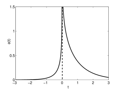
Figure 1: Graph of the function $\phi\left(t\right)$ (Eq.(12))

This logarithmic screening of the Coulomb potential results from a creation of electron-hole pairs in the vicinity of the impurity, or, in terms of quantum electrodynamics (QED), a “vacuum polarization”blp ; migdal . This effect can be qualitatively described in QED by an approach which is very similar to the Thomas-Fermi theory used heremigdal .

As a result, at distances much larger than the lattice constant charge-impurity potential in undoped graphene equals

$$V\left(r\right)\simeq\frac{e^{2}}{\epsilon r}\frac{1}{Q\ln\frac{r}{a}},$$ (14)

does not depend on the impurity charge $Z$ and is much weaker than the bare potential $V_{0}\left(r\right).$ This follows from the fact that the “effective fine-structure constant” for graphene, $\alpha$ is close to 1, instead of 1/137 in QED.

Consider now a generic case of doped graphene. In this case, Eqs.(1), (3), (4), and (6) result in the following integral equation for the total impurity potential:

$$V\left(\mathbf{r}\right)+\frac{2\left|\mu\right|e^{2}}{\pi\epsilon\hbar^{2}v_{F}^{2}}\int d\mathbf{r}^{\prime}\frac{V\left(\mathbf{r}^{\prime}\right)}{\left|\mathbf{r-r}^{\prime}\right|}=\frac{Ze^{2}}{\epsilon r}-\frac{e^{2}}{\pi\epsilon\hbar^{2}v_{F}^{2}}\int\limits_{r^{\prime}>a}d\mathbf{r}^{\prime}\frac{V^{2}\left(\mathbf{r}^{\prime}\right)}{\left|\mathbf{r-r}^{\prime}\right|}$$ (15)

If one neglect the nonlinear term in the right-hand side of Eq.(15) this equation can be easily solved by the Fourier transform; the result for the Fourier component of the total potential, $v\left(q\right)$ readsnomura ; ando

$$v\left(q\right)=\frac{2\pi Ze^{2}}{\epsilon\left(q+\kappa\right)}$$ (16)

where

$$\kappa=\frac{4e^{2}\left|\mu\right|}{\epsilon\hbar^{2}v_{F}^{2}}$$ (17)

is the inverse screening radius proportional to the Fermi wave vector $k_{F}$. After inverse Fourier transformation one finds

$$V\left(r\right)=\frac{Ze^{2}}{\epsilon r}\left\{1-\frac{\pi\kappa r}{2}\left[\mathbf{H}_{0}\left(\kappa r\right)-Y_{0}\left(\kappa r\right)\right]\right\}$$ (18)

with asymptotic behavior

$$V\left(r\right)\simeq\frac{Ze^{2}}{\epsilon r}\frac{1}{\left(\kappa r\right)^{2}}$$ (19)

at $\kappa r\gg 1$; here $\mathbf{H}_{0}$ and $Y_{0}$ are Struve and Neumann functions.

Estimating different terms in Eq.(15) one can demonstrate that the solution (13) is still correct for $\kappa r\leq 1$ and the solution (18) - for $\kappa r\gg 1,$ but with a replacement of $Z$ by

$$Z^{\ast}=Z-\frac{1}{\pi\hbar^{2}v_{F}^{2}}\int\limits_{r^{\prime}>a}d\mathbf{r}^{\prime}V^{2}\left(\mathbf{r}^{\prime}\right)$$ (20)

in the latter case. Analyzing contributions to the integral in the right-hand side of Eq.(19) from these two regions we obtain our final result

$$Z^{\ast}\simeq\frac{Z}{1+ZQ\ln\frac{1}{\kappa a}}.$$ (21)

This is the effective charge of impurity in graphene at distances much larger than the lattice constant. Since we always have $k_{F}a\ll 1$ this means that it is the charge that determines electron scattering by a long-range part of charge impurity potential in graphene. This weakens essentially this scattering mechanism since $Q\ln\frac{1}{\kappa a}$ is of order of ten for typical charge carrier concentrations. Perturbative estimations of the electron mobilitynomura should be thus multiplied by this factor squared. As a result, the mobility for the same parameters turns out to be two order of magnitude larger. Instead of concentration-independent mobility, we obtain a mobility proportional to $\ln^{2}\left(k_{F}a\right)$. This weak dependence on the charge-carrier concentration is probably consistent with the experimental dataprivate . More accurately, one should use an expression for the mobility obtained by Andoando (see Eq.(3.27) and Fig. 5 of that paper) but with the replacement of $Z$ by $Z^{\ast}$ when calculating the strength of the Coulomb interaction.

I am thankful to Andre Geim and Kostya Novoselov for valuable discussions stimulating this work.

References

- (1) K. S. Novoselov, D. Jiang, F. Schedin, T. J. Booth, V. V. Khotkevich, S. M. Morozov, and A. K. Geim, PNAS 102, 10451 (2005).
- (2) K. S. Novoselov, A. K. Geim, S. V. Morozov, D. Jiang, Y. Zhang, S. V. Dubonos, I. V. Grigorieva, and A. A. Firsov, Science 306, 666 (2004).
- (3) K. S. Novoselov, A. K. Geim, S. V. Morozov, D. Jiang, M. I. Katsnelson, I. V. Grigorieva, S. V. Dubonos, and A. A. Firsov, Nature 438, 197 (2005).
- (4) Y. Zhang, Y.-W. Tan, H. L. Stormer, and P. Kim, Nature 438, 201 (2005).
- (5) V. P. Gusynin and S. G. Sharapov, Phys. Rev. Lett. 95, 146801 (2005).
- (6) N. M. R. Peres, F. Guinea, and A. H. Castro Neto, Phys. Rev. B 73, 125411 (2006).
- (7) A. H. Castro Neto, F. Guinea, and N. M. R. Peres, Phys. Rev. B 73, 205408 (2006).
- (8) D. A. Abanin, P. A. Lee, and L. S. Levitov, Phys. Rev. Lett. 96, 176803 (2006).
- (9) M. I. Katsnelson, Eur. Phys. J. B 51, 157 (2006).
- (10) J. Tworzydlo, B. Trauzettel, M. Titov, A. Rycerz, and C. W. J. Beenakker, Phys. Rev. Lett. 96, 246802 (2006).
- (11) K. Ziegler, cond-mat/0604537.
- (12) K. Nomura and A. H. MacDonald, Phys. Rev. Lett. 96, 256602 (2006).
- (13) T. Ando, J. Phys. Soc. Japan 75, 074716 (2006).
- (14) T. Ando, A. B. Fowler, and F. Stern, Rev. Mod. Phys. 54, 437 (1982).
- (15) P. Hohenberg and W. Kohn, Phys. Rev. 136, B884 (1964).
- (16) E. H. Lieb, Rev. Mod. Phys. 53, 603 (1981).
- (17) D. Pines and P. Nozieres, The Theory of Quantum Liquids, Vol. 1 (Benjamin, Massachusetts, 1966).
- (18) S. V. Vonsovsky and M. I. Katsnelson, Quantum Solid State Physics (Springer, New York, 1989), Chap. 5.
- (19) E. M. Lifshitz and L. P. Pitaevskii, Relativistic Quantum Theory, Part 2 (Pergamon, Oxford etc., 1977).
- (20) A. B. Migdal, Qualitative Methods in Quantum Theory (Benjamin, Reading, Mass., 1977).
- (21) A. K. Geim and K. S. Novoselov, private communication.