Capillary wave dynamics on supported viscoelastic films: Single and double layers

Abstract

We study the capillary wave dynamics of a single viscoelastic supported film and of a double layer of immiscible viscoelastic supported films. Using both simple scaling arguments and a continuum hydrodynamic theory, we investigate the effects of viscoelasticity and interfacial slip on the relaxation dynamics of these capillary waves. Our results account for the recent observation of a wavelength-independent decay rate for capillary waves in a supported polystyrene/brominated polystyrene double layer [X. Hu et al., Phys. Rev. E 74, 010602 (R) (2006)].

I Introduction

Due to the presence of thermally excited capillary waves, the free surfaces of fluids lamb:32 , complex fluids, and other generically soft materials are fluctuating structures. Examining the surface dynamics of such soft materials provides a window into their rheology. Consequently, capillary waves and interfacial dynamics have been probed by light scattering techniques hard:87 ; hughes:93 in a variety of systems, including membranes and monolayers kramer:71 , liquid metals earnshaw:82 , and polymer solutions huang:96 ; munoz:05 , brushes kim:05 , and gels langevin:98 . These light scattering techniques probe surface dynamics at length scales in the micron range; however, newer experiments using x-ray photon correlation spectroscopy (XPCS) thurn:96 ; gutt:03 extend these measurements into the sub-micron range, allowing investigators to probe even smaller scale surface height fluctuations.

The theory of the surface dynamics of polymeric materials has focused on the continuum mechanics of viscoelastic liquids, including two-fluid approaches to semi-infinite polymer solutions harden:91 and single component fluids supported on a rigid substrate jackle:98 ; rauscher:05 ; kumaran:92 . These continuum approaches have been remarkably successful in accounting for the surface dynamics observed experimentally in many systems. In polymeric systems such continuum based methods must begin to fail in the limit of increasing molecular weight and decreasing film thickness, where the short dimension of the liquid becomes comparable to size of the constituent molecules. Indeed, there is experimental evidence keddie:94 for and subsequent theoretical conjecture degennes:00 ; mccoy:02 about the shift (relative to its bulk value) in the glass transition temperature of high molecular weight polymer thin films.

In recent experiments Lal, Sinha, and coworkers kim:03 ; lal:05 used XPCS to study capillary waves on layers of polymeric films. They examined both single layers of polystyrene (PS) supported on a silicon substrate kim:03 and double layers of a PS layer overlying a brominated polystyrene (PBrS) layer on a silicon substrate lal:05 . In the double layer experiments, the XPCS technique allowed for the independent measurement of the dynamics of both the upper surface of the PS, which we refer to as the free surface, and the PS/PBrS interface, which we refer to as the buried interface.

The most striking result of the Lal et al. double layer experiments is the appearance of a slow ($\sim 100$ s) decay rate in the height-height correlations of both the upper and buried interfaces that is approximately independent of the in-plane wave number $q$. Such a phenomenon cannot be explained by previous theoretical work harden:91 ; jackle:98 ; rauscher:05 ; kumaran:92 . In this article we extend the previous theoretical work to two-layer viscoelastic systems and explore – via continuum visco-hydrodynamic calculations and scaling arguments – the possible origins of the $q$-independent decay rate reported by Lal and collaborators. Acknowledging that the thickness of the fluid layers is on the order of a few radii of gyration of the constituent molecules, one may question whether these discrepancies point towards the failure of a continuum-based analysis. Despite this concern, we show that a viscoelastic continuum model can give rise to the observed $q$-independent decay rate. In order to quantitatively account for the experimental data, however, we must use surprisingly long stress relaxation times in these continuum models, which in turn leads us to postulate that the polymer dynamics in the thin films is hindered by confinement effects. Based on these attempts to fit the scattering data using our model, we suggest that the experiments provide an interesting measure of confinement effects on the molecular dynamics in the melt.

The remainder of the paper is organized as follows: in section II we examine simple scaling arguments that suggest that viscoelastic supported films can exhibit the phenomena reported by Lal and collaborators. In section III we calculate the dynamics of the single supported fluid layer system using a continuum hydrodynamic description of the fluid. We consider both a purely viscous Newtonian fluid and the simplest model for a viscoelastic fluid, the Maxwell fluid, which is characterized by a single relaxation time. We also examine the effects of slip at the fluid/substrate interface on these dynamics; in particular, we show that slip alone cannot account for the $q$-independent decay rate. We then turn to the study of the two layer system in section IV. Here, we consider both the system of two Newtonian fluids as well as the case of one Newtonian fluid and one Maxwell fluid. We show that our model of a Maxwell fluid buried beneath a Newtonian fluid can account for a number of the experimental features observed in the double layer systems studied by Lal et al.. We again explore the effects of slip on the dynamics of the system, in this case at the liquid/liquid interface. Finally, in section V, we discuss our results more broadly in the context of the dynamics of multilayered systems, focusing on the long stress relaxation times necessary to account for the results of the Lal group, as well as the implications such times have for the dynamics of polymers near an interface. We conclude with suggestions for future experiments to further test our analysis.

II Scaling Analysis

The experiments of Lal et al. kim:03 ; lal:05 present an interesting theoretical challenge for which at least a few suggestions have been offered harden:91 ; jackle:98 ; rauscher:05 . We first use a few numerical estimates to narrow the focus of our problem. Consider a supported fluid film of thickness $d$ on a solid substrate, as shown in Fig. 1. The fluid has mass density $\rho$ and a surface tension $\gamma$ at the free surface. The deformation of the free surface in capillary waves is subject to restoring forces due to gravity and surface tension. We assume that the bending energies of the interface are negligible (we will return briefly to this point in section V). The importance of these two forces depends strongly on the wavelength of the disturbance. For wavelengths less than the capillary length $\sqrt{\gamma/\rho g}$, surface tension induced forces dominate over gravitational forces. The XPCS experiments can detect capillary waves of wavelengths less than the typical transverse coherence length of the beam, which is $\sim 10\mu$m  kim:03 ; gutt:03 ; lal:05 . The capillary wavelength, however, is on the order of $1$ cm; therefore, we may neglect the effect of gravity.

The importance of inertial effects in the fluid dynamics may be estimated by considering the Reynolds number landau:04 of the flows associated with the capillary waves. The Reynolds number for such flows is given by $\mbox{Re}\sim D_{1}h\omega/\nu$, where $D_{1}$ is the length scale over which the fluid velocity vanishes (we expect it to the be the lesser of the inverse wave number $1/q$ and the film thickness $d$), $\nu=\eta/\rho$ is the kinematic viscosity and $h$, $\omega$ are the typical height and decay rate of the surface disturbance, respectively. Using the equipartition theorem to determine the average magnitude of thermally generated capillary waves, $\langle|h_{q}|^{2}\rangle\sim k_{\rm B}T/\gamma q^{2}$, we find that $\mbox{Re}\sim{\mathcal{O}}(10^{-7})$. This estimate demonstrates that inertial stresses are greatly dominated by viscous ones in the material. Thus, we ignore inertial stresses in the remainder of this article; that is, we assume that all of the fluids are completely overdamped.

Given that we are considering low Reynolds number dynamics at scales well below the capillary length, we now turn to simple scaling arguments to determine the possible wave number dependence of the relaxation rates of overdamped capillary waves. In particular, we ask: what properties of the fluid lead to a $q$-independent dispersion relation, i.e. $\omega(q)\sim q^{0}$? The fluid deformations generated by capillary waves store energy in the fluid interface and, for viscoelastic fluids, in the bulk as well. When these deformations relax, this energy is dissipated through viscous stresses in the fluid. The scaling behavior of the dispersion relation can then be found by equating the power generated by relaxing the elastic deformations in the fluid with the power dissipated viscously by the fluid.

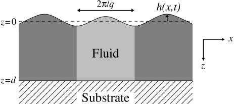
Figure 1: Schematic illustration of a single supported fluid layer of thickness $d$.

For a Newtonian fluid, energy can be stored only in the interface at the free surface. Consider the lightly shaded portion of the fluid in Fig. 1, whose cross-sectional area in the $x-y$ plane is $A\sim l/q$, $l$ being a unit length in the ${\bf\hat{y}}$ direction. The total power transferred to this volume of fluid from the interface is the product of the normal stress generated by the surface tension $\gamma q^{2}h$, the surface area $A$, and speed of the surface as the deformation relaxes, $\omega h$:

$$P_{surf}\sim\left(\gamma q^{2}h\right)A\omega h.$$ (1)

The viscous force density for the incompressible fluid is $\eta\nabla^{2}v$, where $v$ is the fluid velocity. Then the power dissipated in the bulk of the fluid is given by

$$P_{diss}=\int d^{3}\!x\,v\eta\nabla^{2}v\approx A\eta\int_{0}^{d}d\!z\,\bar{v}(z)\nabla^{2}\bar{v}(z),$$ (2)

where $\bar{v}(z)$ is velocity averaged over one wavelength in the horizontal (${\bf\hat{x}}$) direction; since the velocity is periodic in $x$, its variation in $x$ does not affect the scaling behavior of the dispersion relation.

We can relate the fluid velocity $\bar{v}$ to the interfacial height via volume conservation. During the relaxation of a surface undulation, fluid volume is transferred from elevated regions to the depressed ones, so $A\partial_{t}h\approx\int d\!yd\!z\bar{v}(z)$, where the integral is over a unit of area whose normal is parallel to ${\bf\hat{x}}$. Using this relation and equating the power input to the power dissipated, we find that the wave number dependence of the decay rate $\omega$ can be determined from

$$\omega\sim\frac{\gamma q^{4}\left[\int_{0}^{d}d\!z\bar{v}(z)\right]^{2}}{\eta\int_{0}^{d}d\!z\bar{v}(z)\nabla^{2}\bar{v}(z)}.$$ (3)

We now distinguish two different scaling regimes. In the thin layer limit ($qd\ll 1$) the velocity decay into the fluid is set by the thickness of the layer, so $\int_{0}^{d}d\!z\sim d$ and $\nabla^{2}\sim 1/d^{2}$. For thick layers ($qd\ll 1$), however, the velocity decays exponentially into the fluid, so $\int_{0}^{d}d\!z\sim 1/q$ and the $\nabla^{2}\sim q^{2}$. Thus, we find two possible dispersion relations depending on the the value of $qd$,

$$\omega\sim\begin{cases}\frac{\gamma q^{4}d^{3}}{\eta}&qd\ll 1\\ \frac{\gamma q}{\eta}&qd\gg 1\end{cases}.$$ (4)

This argument suggests that a Newtonian fluid will not exhibit the desired $q$-independent dispersion relation.

If we consider instead a viscoelastic fluid, we note that elastic energy is also stored in the bulk due to the state of deformation in the material, as long as the decay rate of the capillary wave is fast compared to the stress relaxation time in the viscoelastic material. This storage of elastic energy in the bulk changes our previous scaling arguments. For example, in an elastic solid characterized by a bulk modulus $\mu$, the power released in the bulk during the relaxation of the deformation takes the form

$$P_{bulk}\sim A\mu\int_{0}^{d}\bar{v}(z)\nabla^{2}\bar{u}(z),$$ (5)

where $\bar{u}(z)$ is the average displacement field in the medium: $\bar{u}(z)\sim\bar{v}(z)/\omega$. This expression is similar in form to the viscous power dissipation in Eq. (2). Indeed, if we equate the power dissipated with the power input from the bulk, we find $\omega\sim\mu/\eta$ for all values of $q$. Thus, this simple scaling argument suggests that the desired $q$-independent behavior is a manifestation of the viscoelastic response of the fluid. In order to verify the results of these heuristic arguments, and to determine over which range of wave numbers one might observe a $q$-independent dispersion relation, we now turn to the complete solutions of the Stokes equation for supported, overdamped Newtonian and viscoelastic fluid layers.

III Single Layer

Consider the response of the single, supported, incompressible fluid layer shown in Fig. 1 to an external stress field $\sigma^{ext}$, which is normal to the free surface and characterized by frequency $\omega$ and wave vector ${\bf q}\equiv q{\bf\hat{x}}$,

$$\sigma^{ext}=\sigma_{0}e^{i\left(qx-\omega t\right)}.$$ (6)

The response of the fluid to the applied stress is described by the vertical deviation or height function of the free surface $h(x,t)$, the velocity ${\bf v}(x,z,t)$, and the pressure $P(x,z,t)$. Given the form of $\sigma^{ext}$ in Eq. (6), all of these dynamical quantities can be written in the form

$$g(x,z,t)=g(q,z,\omega)e^{i\left(qx-\omega t\right)}.$$ (7)

The general solution to the Stokes equation in the case that the dynamical quantities take the form of Eq. (7) is determined in Appendix A. In particular, all of the dynamical quantities listed above can be related to the normal component of the fluid velocity, which is given by Eq. (65). In order to determine the four integration constants in Eq. (65), we need to specify the boundary conditions at the top and bottom boundaries of the fluid. At the fluid/substrate interface, the normal component of the fluid velocity must vanish,

$$\left.v_{z}\right|_{z=d}=0.$$ (8)

We may account for both slip and stick boundary conditions on the tangential velocity component by introducing a slip length $\lambda$, so that at the fluid/substrate interface

$$\left.v_{x}\right|_{z=d}=-\lambda\left.\partial_{z}v_{x}\right|_{z=d}.$$ (9)

Taking $\lambda=0$ reduces the above boundary condition to the usual no-slip condition.

At the free surface, the rate of change of the height of the interface must equal the fluid velocity at that point,

$$\left.v_{z}\right|_{z=0}=-i\omega h(q,\omega).$$ (10)

Furthermore, this interface cannot support shear stresses,

$$\left.\sigma_{xz}^{f}\right|_{z=0}=0,$$ (11)

where the fluid stress tensor $\sigma^{f}$ takes the usual form,

$$\sigma_{ij}^{f}=\eta(\omega)\left(\partial_{i}v_{j}+\partial_{j}v_{i}\right)-\delta_{ij}P,$$ (12)

$\eta(\omega)$ being the frequency dependent viscosity characterizing the viscoelastic response of the material. Finally, the free surface can support a stress discontinuity between the externally applied stress and the hydrodynamic stresses in the bulk material, due to the presence of a finite surface tension:

$$\sigma^{ext}=\gamma q^{2}h(q,\omega)-\left.\sigma_{zz}^{f}\right|_{z=0}.$$ (13)

Using the boundary conditions Eqs. (8)-(11) to solve for the fluid velocity and pressure fields, we obtain the normal fluid stress at the free surface from Eq. (12),

$$\left.\sigma_{zz}^{f}\right|_{z=0}=i\omega\eta(\omega)B(q)h(q,\omega),$$ (14)

where

$$B(q)=4q\frac{\cosh^{2}(qd)+q^{2}d^{2}+q\lambda\left(2qd+\sinh(2qd)\right)}{\sinh(2qd)-2qd+4q\lambda\sinh^{2}(qd)}.$$ (15)

Then Eq. (13) becomes

$$\sigma_{0}=h(q,\omega)\left[\gamma q^{2}-i\omega\eta(\omega)B(q)\right].$$ (16)

The normal mode frequencies are those which satisfy Eq. (16) in the absence of an external stress and with a non-zero fluid height:

$$\gamma q^{2}-i\omega_{n}\eta(\omega_{n})B(q)=0.$$ (17)

For this overdamped system the frequencies $\omega_{n}$, given by the solutions to Eq. (17), all lie on the negative imaginary axis. We refer to the norm of these complex numbers as the decay rates of the system, $\tilde{\omega}_{n}=i\omega_{n}$.

The experimentally measurable quantity for this system is the intensity autocorrelation function, which is directly proportional to the height-height correlation function $S(q,t)\propto\left<h(q,t)h^{*}(q,0)\right>$ (see Appendix B for further details). Using Eq. (68), we find the height-height correlation function to be

$$S(q,t)=-\sum_{\omega_{n}}\lim_{\omega\rightarrow\omega_{n}}\frac{\left(\omega-\omega_{n}\right)e^{-i\omega t}}{\omega\left[\gamma q^{2}-i\omega\eta(\omega)B(q)\right]}.$$ (18)

Thus, the surface height dynamics – as parameterized by the decay rates $\tilde{\omega}_{n}$ – can be extracted from the experimental measurement of $S(q,t)$. We now turn to the calculation of these decay rates for single supported Newtonian and Maxwell fluids. In light of the Lal et al. data we pay particular attention to the dependence of these decay rates on wave number $q$.

III.1 Newtonian Fluid

For Newtonian fluid the viscosity is real, positive, and independent of frequency, $\eta(\omega)=\eta>0$. This is generally a good approximation for small molecule liquids and for viscoelastic materials on time scales much longer than their typical stress relaxation times. As shown in Appendix C, we expect only one decay rate, and indeed there is only one root of Eq. (17) in this case,

$$\tilde{\omega}(q)=\frac{\gamma q^{2}}{\eta B(q)}.$$ (19)

We note that, for the case where there is no slip between the fluid and substrate, the same result can be obtained from the previous theoretical work of Jäckle jackle:98 ; kim:03 .

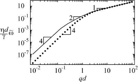
Figure 2: Dimensionless decay rate $\eta d\tilde{\omega}/\gamma$ for a Newtonian fluid as a function of $qd$. The solid (dotted) lines are for a system with a small (large) liquid/substrate slip length, $\lambda=0.01d$ ($\lambda=10d$).

The decay rates in the presence of both small and large slip lengths are shown in Fig. 2. When the slip length is small, $\lambda\ll d$, the decay rate is independent of it to leading order in $q$,

$$\tilde{\omega}(q)=\begin{cases}\frac{\gamma q^{4}d^{3}}{3\eta}&qd\ll 1\\ \frac{\gamma|q|}{2\eta}&qd\gg 1\\ \end{cases}.$$ (20)

Other than numerical prefactors, this result is identical to the one obtained using the simple scaling arguments given above – see Eq. (4). It is also consistent with the experimental results obtained by Sinha et. al for a single PS layer, for which a $q^{4}$ scaling behavior was observed over wave numbers $qd<1$ kim:03

When a significant amount of slip occurs between the fluid and the solid interface (i.e. $\lambda\gg d$), an intermediate scaling regime in the decay rate appears,

$$\tilde{\omega}(q)=\begin{cases}\frac{\gamma q^{4}d^{2}\lambda}{\eta}&qd\ll 1,\,q^{2}d\lambda\ll 1\\ \frac{\gamma q^{2}d}{4\eta}&qd\ll 1,q^{2}d\lambda\gg 1\\ \frac{\gamma|q|}{2\eta}&qd\gg 1\end{cases}.$$ (21)

Thus, we can see that a Newtonian fluid does not exhibit a $q$-independent decay rate, even if there is a significant amount of slip between the fluid and substrate.

Because there is only one decay rate, the height-height correlation function Eq. (18) exhibits a simple exponential decay,

$$S(q,t)=\frac{1}{\gamma q^{2}}e^{-\tilde{\omega}t}.$$ (22)

III.2 Maxwell Fluid

A Maxwell fluid, which is the simplest model for a viscoelastic material, has a complex, frequency dependent viscosity of the form

$$\eta(\omega)=\eta+\frac{E\tau}{1-i\omega\tau},$$ (23)

where $E$ is the transient modulus of the polymer network, $\tau$ is the stress relaxation time of the medium, and $\eta$ accounts for the high frequency viscous response landau:elasticity . In this case Eq. (17) can be written as a quadratic equation in $\omega$; that is, we obtain two decay rates, in agreement with the arguments given in Appendix C. These rates are given by

$$\tilde{\omega}_{\pm}(q)=\frac{\mathcal{N}\pm\sqrt{\mathcal{N}^{2}-4\beta\eta\tau}}{2\eta\tau},$$ (24)

where $\mathcal{N}\equiv\eta+E\tau+\beta\tau$ and $\beta(q)=\gamma q^{2}/B(q)$. Since $\mathcal{N}^{2}-4\beta\eta\tau=\left(\eta+E\tau-\beta\tau\right)^{2}+4\beta E\tau^{2}>0$ both the fast decay rate $\tilde{\omega}_{+}$ and slow decay rate $\tilde{\omega}_{-}$ are positive real numbers.

Parameter	symbol	Value
PS layer thickness	$d_{2}$	$100$ nm
PBrS layer thickness	$d$ [SL], $d_{1}$ [DL]	$200$ nm
PS viscosity	$\eta_{2}$	$10^{4}$ kg/m$\cdot$s
PBrS viscosity	$\eta$ [SL], $\eta_{1}$ [DL]	$10^{6}$ kg/m$\cdot$s
PBrS surface tension [SL]	$\gamma$	$10^{-2}$ N/m
Interface tension PS/PBrS	$\gamma_{1}$	$10^{-3}$ N/m
PS surface tension	$\gamma_{2}$	$10^{-2}$ N/m
PBrS Plateau modulus	$E$	$10^{3}$ Pa
PBrS stress relaxation time	$\tau$	$100$ s

Table 1: Geometric and rheological parameters corresponding to the single layer [SL] and double layer [DL] Lal experiments lal:05 . Both the plateau modulus and the stress relaxation time are chosen so as to reproduce the major features observed experimentally in the double layer system (see section IV).

In Fig. 3 we plot the fast and slow decay rates for both small and large amounts of slip at the substrate, using parameter values characteristic of a layer of PBrS, as listed in Table 1. When the slip length is small compared to the film thickness, $\lambda\ll d$, we find

$$\tilde{\omega}_{+}(q) =\begin{cases}\frac{\eta+E\tau}{\eta\tau}&qd\ll 1\\ \frac{\gamma|q|}{2\eta}&qd\gg 1\end{cases},$$ (25)

$$\tilde{\omega}_{-}(q) =\begin{cases}\frac{\gamma q^{4}d^{3}}{3\left(\eta+E\tau\right)}&qd\ll 1\\ \frac{1}{\tau}&qd\gg 1\end{cases}.$$ (26)

When the slip length is large compared to film thickness, $\lambda\gg d$, we find

$$\tilde{\omega}_{+}(q) =\begin{cases}\frac{\eta+E\tau}{\eta\tau}&qd\ll 1\\ \frac{\gamma|q|}{2\eta}&qd\gg 1\end{cases},$$ (27)

$$\tilde{\omega}_{-}(q) =\begin{cases}\frac{\gamma q^{4}d^{2}\lambda}{\eta+E\tau}&qd\ll 1,\,q^{2}d\lambda\ll 1\\ \frac{\gamma q^{2}d}{4\left(\eta+E\tau\right)}&qd\ll 1,\,q^{2}d\lambda\gg 1\\ \frac{1}{\tau}&qd\gg 1\end{cases}.$$ (28)

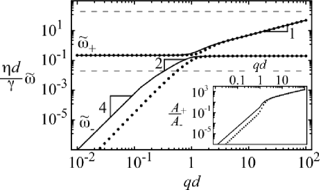
Figure 3: Dimensionless decay rates $\eta d\tilde{\omega}_{\pm}/\gamma$ for a Maxwell fluid as a function of $qd$, using the parameter values listed in Table 1 for PBrS. The solid (dotted) lines are for a system with a small (large) liquid/substrate slip length, $\lambda=0.01d$ ($\lambda=10d$). The dashed lines indicate the approximate window of decay rates that can be measured in the experiments, $10^{-3}s^{-1}<\tilde{\omega}<10s^{-1}$. Inset: Ratio of the amplitude of the term in $S(q,t)$ that decays with rate $\tilde{\omega}_{+}$ to that of the term that decays with rate $\tilde{\omega}_{-}$.

As we can see from both the analytic expressions and the numerical results shown in Fig. 3, the fast (slow) decay rate is independent of $q$ at low (high) wave numbers. Such behavior is in agreement with the experimental results of Lal et al., and it is also consistent with the scaling arguments given in section II for the elastic response of a viscoelastic fluid. On the other hand, the scaling of the fast and slow decay rates in their respective $q$-dependent regimes – at high $qd$ in the former case, and at low $qd$ in the latter – is identical to that of a Newtonian fluid in these regimes. Thus, the viscous response of the fluid determines the scaling of $\tilde{\omega}_{\pm}$ where each decay rate exhibits a strong dependence on the wavelength, whereas the elastic response of the fluid gives rise to the $q$-independent behavior of $\tilde{\omega}_{\pm}$.

From this analysis we predict that the height-height correlation function $S(q,t)$ will exhibit a double exponential decay for a Maxwell fluid. In particular, Eq. (68) becomes

$$S(q,t)= \sum_{\pm}\left[\frac{\left(\tilde{\omega}_{\pm}\tau-1\right)}{\eta\tau B(q)\tilde{\omega}_{\pm}\left(\tilde{\omega}_{\pm}-\tilde{\omega}_{\mp}\right)}\right]e^{-\tilde{\omega}_{\pm}t}$$ (29)

$$\equiv \sum_{\pm}A_{\pm}e^{-\tilde{\omega}_{\pm}t}.$$

These amplitudes are plotted in the inset of Fig. 3.

In order to predict the form of experimental measurements of $S(q,t)$, one must consider the values of both the decay rates and the $q$-dependent amplitudes appearing in Eq. (29). In principle, the decay of the height-height correlation function $S(q,t)$ should always have the double exponential form given in Eq. (29). It is clear from the inset of Fig. 3, however, that the amplitude of one of these terms can dominate the other at certain wave numbers. In particular, the amplitude of the slow mode dominates for $qd\ll 1$, whereas the amplitude of the fast mode dominates for $qd\gg 1$. In these regimes, it will be hard to measure both decay rates. The full double exponential decay should be observable only in the crossover region between these two regimes, which occurs at $qd\sim 1$ for parameter values consistent with current experiments.

We can see from the inset of Fig. 3 that for both $qd\ll 1$ and $qd\gg 1$, the amplitude of the $q$-dependent rate is much larger than that of the $q$-independent rate. Taken in isolation, this fact suggests that it would be difficult to observe the $q$-independent rate in these regions. In predicting the experimentally observed behavior of $S(q,t)$, however, it is important to take the value of the decay rates themselves into account. In particular, there is a finite range of decay rates that can be measured: the decay times can be too fast or too slow to be observed within the time scales of the experiment. We have indicated a reasonable experimental window – from $1/10$ sec to $1000$ sec for the decay times – by the dashed lines in Fig 3. Then we see, for example, that the slow decay rate becomes too slow to be measured experimentally at long wavelengths. As a result, the faster $q$-independent decay rate could be observed in this regime, despite the fact that its amplitude is much smaller than the slow decay rate. We do not comment on the sensitivity of the experiments to small amplitude capillary dynamics. If the larger amplitude mode is too slow and the smaller amplitude mode generates too small a surface height undulation, no interfacial dynamics may be detected.

This analysis suggests that for $qd<1$ it should in principle be possible to observe a $q$-independent decay of $S(q,t)$ over at least one decade of $qd$, depending on the sensitivity of the measurement. For higher wave numbers, $qd>1$, however, we expect this $q$-independent behavior to be obscured by the slower $q$-dependent mode with a larger amplitude, since it will then be fast enough to be measured by the current experiments.

IV Double Layer

Figure 4: Schematic illustration of two fluid layers, of thicknesses $d_{1}$ and $d_{2}$, on a substrate. The coordinates are chosen so that the fluid/solid interface is the plane $z=d$ and the unperturbed free surface is the plane $z=0$.

We now turn to the double layer case, illustrated in Fig. 4. The buried and upper fluids have viscosities $\eta_{1}(\omega),\eta_{2}(\omega)$ and thicknesses $d_{1},d_{2}$, respectively. The total thickness is $d=d_{1}+d_{2}$. In general, we can drive this system by spatially oscillatory normal stresses acting on both the buried fluid/fluid interface and the free surface. As in the single layer case, we consider stresses of the form of Eq. (6). Combining the stresses on both interfaces into a single vector, we write

$$\bm{\sigma^{ext}}(x,t)=\begin{bmatrix}\sigma_{1}\\ \sigma_{2}\\ \end{bmatrix}e^{i\left(qx-\omega t\right)}.$$ (30)

For simplicity, we consider the possibility of slip at only the fluid/fluid interface, as the effects of slip at the fluid/substrate interface have already been explored in the single layer case.

At the fluid/substrate interface all components of the fluid velocity must vanish:

$$\left.v_{1,z}\right|_{z=d}=\left.v_{1,x}\right|_{z=d}=0.$$ (31)

At the fluid/fluid interface the $z$-components of the velocities of the two fluids must match, but the tangential components of the velocities do not if there is a finite slip length $\lambda$ at this interface:

$$\left.v_{1,z}\right|_{z=d_{2}} = \left.v_{2,z}\right|_{z=d_{2}},$$ (32)

$$\left.\left(v_{2,x}-v_{1,x}\right)\right|_{z=d_{2}} = -\lambda\left.\left(\partial_{z}v_{2,x}-\partial_{z}v_{1,x}\right)\right|_{z=d_{2}}.$$ (33)

Note that $\lambda>0$ when the buried polymer layer is more viscous than the upper layer ($\mbox{Re}\left[\eta_{1}(\omega)\right]>\mbox{Re}\left[\eta_{2}(\omega)\right]$ for all real $\omega$), and vice-versa.

From the definition of the interface heights,

$$\left.v_{1,z}\right|_{z=d_{2}} = -i\omega h_{1}(q,\omega),$$ (34)

$$\left.v_{2,z}\right|_{z=0} = -i\omega h_{2}(q,\omega).$$ (35)

In addition, the free surface cannot support shear stresses, and the shear stress must be continuous across the fluid/fluid interface:

$$\left.\sigma_{2,xz}^{f}\right|_{z=0} = 0,$$ (36)

$$\left.\sigma_{1,xz}^{f}\right|_{z=d_{2}} = \left.\sigma_{2,xz}^{f}\right|_{z=d_{2}}.$$ (37)

Finally, the normal stress discontinuities at both the fluid/fluid interface and the free surface are determined by their respective surface tensions ($\gamma_{1}$ and $\gamma_{2}$, respectively),

$$\sigma_{1} = \gamma_{1}q^{2}h_{1}(q,\omega)-\left[\sigma_{2,zz}^{f}-\sigma_{1,zz}^{f}\right|_{z=d_{2}},$$ (38)

$$\sigma_{2} = \gamma_{2}q^{2}h_{2}(q,\omega)-\left.\sigma_{2,zz}^{f}\right|_{z=0}.$$ (39)

Using Eqs. (31)– (37) to eliminate the fluid velocities in favor of the interfacial height functions, the normal stress equations Eqs. (38) and  (39) can be written in matrix form:

$$\bm{\sigma}=\bm{\Sigma}\cdot\bm{h},$$ (40)

where $\bm{\sigma}\equiv\begin{bmatrix}\sigma_{1}\\ \sigma_{2}\\ \end{bmatrix}$, $\bm{h}\equiv\begin{bmatrix}h_{1}(q,\omega)\\ h_{2}(q,\omega)\\ \end{bmatrix}$, and

$$\bm{\Sigma}\equiv\begin{bmatrix}\gamma_{1}q^{2}-\frac{i\omega s_{11}(q,\omega)}{\Delta(q,\omega)}&-\frac{i\omega s_{12}(q,\omega)}{\Delta(q,\omega)}\\ -\frac{i\omega s_{12}(q,\omega)}{\Delta(q,\omega)}&\gamma_{2}q^{2}-\frac{i\omega s_{22}(q,\omega)}{\Delta(q,\omega)}\\ \end{bmatrix},$$ (41)

with

$$s_{11}(q,\omega)= 4q\eta_{1}^{2}\left[1+\left(1+2q^{2}d_{1}^{2}\right)\,\mbox{sech}\left(2qd_{1}\right)\right]\left[\tanh\left(2qd_{2}\right)-2qd_{2}\,\mbox{sech}\left(2qd_{2}\right)\right]+4q\eta_{2}^{2}\left[1-\left(1+2q^{2}d_{1}^{2}\right)\,\mbox{sech}\left(2qd_{1}\right)\right]$$

$$*\left[\tanh\left(2qd_{2}\right)+2qd_{2}\,\mbox{sech}\left(2qd_{2}\right)\right]+8q\eta_{1}\eta_{2}\left[2qd_{1}\left(2q^{2}d_{1}d_{2}-1\right)\,\mbox{sech}\left(2qd_{1}\right)\,\mbox{sech}\left(2qd_{2}\right)+\tanh\left(2qd_{1}\right)\right]$$

$$+8q^{2}\lambda\left(\eta_{1}-\eta_{2}\right)\Big{\{}\eta_{1}\left[1+\left(1+2q^{2}d_{1}^{2}\right)\,\mbox{sech}\left(2qd_{1}\right)\right]\left[1-\,\mbox{sech}\left(2qd_{2}\right)\right]\Big{.}$$ (42)

$$\Big{.}+\eta_{2}\left[\tanh\left(2qd_{1}\right)-2qd_{1}\,\mbox{sech}\left(2qd_{1}\right)\right]\left[\tanh\left(2qd_{2}\right)+2qd_{2}\,\mbox{sech}\left(2qd_{2}\right)\right]\Big{\}},$$

$$s_{12}(q,\omega)= -\frac{8q\eta_{2}}{2\cosh\left(qd_{2}\right)-\,\mbox{sech}\left(qd_{2}\right)}\Big{\{}\eta_{2}\left[1-\left(1+2q^{2}d_{1}^{2}\right)\,\mbox{sech}\left(2qd_{1}\right)\right]\left[qd_{2}+\tanh\left(qd_{2}\right)\right]\Big{.}$$

$$+\eta_{1}\Big{[}2q^{3}d_{1}^{2}d_{2}\,\mbox{sech}\left(2qd_{1}\right)+\left[\tanh\left(2qd_{1}\right)-2qd_{1}\,\mbox{sech}\left(2qd_{1}\right)\right]\left[qd_{2}\tanh\left(qd_{2}\right)+1\right]\Big{]}$$ (43)

$$+\Big{.}2q\lambda\left(\eta_{1}-\eta_{2}\right)\left[\tanh\left(2qd_{1}\right)-2qd_{1}\,\mbox{sech}\left(2qd_{1}\right)\right]\left[\tanh\left(qd_{2}\right)+qd_{2}\right]\Big{\}},$$

$$s_{22}(q,\omega)= 4q\eta_{2}^{2}\left[1-\left(1+2q^{2}d_{1}^{2}\right)\,\mbox{sech}\left(2qd_{1}\right)\right]\left[\tanh\left(2qd_{2}\right)+2qd_{2}\sec\left(2qd_{2}\right)\right]$$

$$+4q\eta_{1}\eta_{2}\left[\tanh\left(2qd_{1}\right)-2qd_{1}\,\mbox{sech}\left(2qd_{1}\right)\right]\left[1+\left(1+2q^{2}d_{2}^{2}\right)\,\mbox{sech}\left(2qd_{2}\right)\right]$$ (44)

$$+8q^{2}\lambda\eta_{2}\left(\eta_{1}-\eta_{2}\right)\left[\tanh\left(2qd_{1}\right)-2qd_{1}\,\mbox{sech}\left(2qd_{1}\right)\right]\left[\tanh\left(2qd_{2}\right)+2qd_{2}\,\mbox{sech}\left(2qd_{2}\right)\right],$$

$$\Delta(q,\omega)= 2\eta_{2}\left[1-\left(1+2q^{2}d_{1}^{2}\right)\,\mbox{sech}\left(2qd_{1}\right)\right]\left[1-\,\mbox{sech}\left(2qd_{2}\right)\right]+2\eta_{1}\left[\tanh\left(2qd_{1}\right)-2qd_{1}\,\mbox{sech}\left(2qd_{1}\right)\right]$$ (45)

$$*\left[\tanh\left(2qd_{2}\right)-2qd_{2}\,\mbox{sech}\left(2qd_{2}\right)\right]+4q\lambda\left(\eta_{1}-\eta_{2}\right)\left[\tanh\left(2qd_{1}\right)-2qd_{1}\,\mbox{sech}\left(2qd_{1}\right)\right]\left[1-\,\mbox{sech}\left(2qd_{2}\right)\right],$$

where, for clarity, we have suppressed the (possible) frequency dependence of the viscosities $\eta_{1}$ and $\eta_{2}$.

The two normal modes of the double layer system are easily identified if we diagonalize the normal stress matrix equation Eq. (41), bringing the dynamical relations into the form

$$\begin{bmatrix}\sigma_{+}\\ \sigma_{-}\\ \end{bmatrix}=\begin{bmatrix}\lambda_{+}&0\\ 0&\lambda_{-}\\ \end{bmatrix}\begin{bmatrix}h_{+}(q,\omega)\\ h_{-}(q,\omega)\\ \end{bmatrix},$$ (46)

where

$$\sigma_{\pm}\equiv\Lambda_{1}^{\pm}\sigma_{1}+\Lambda_{2}^{\pm}\sigma_{2},\qquad h_{\pm}\equiv\Lambda_{1}^{\pm}h_{1}+\Lambda_{2}^{\pm}h_{2},$$ (47)

and $\lambda_{\pm}$ and $\Lambda^{\pm}$ are, respectively, the eigenvalues and the orthonormal eigenvectors of the matrix $\bm{\Sigma}$. The eigenvalues may be written as

$$\lambda_{\pm}=\frac{1}{2}\left[\mbox{Tr }\bm{\Sigma}\pm\sqrt{\left(\mbox{Tr }\bm{\Sigma}\right)^{2}-4\det\bm{\Sigma}}\right],$$ (48)

and the corresponding eigenvectors are

$$\bm{\Lambda^{\pm}}=\frac{1}{\sqrt{\Sigma_{12}^{2}+\left(\lambda_{\pm}-\Sigma_{11}\right)^{2}}}\begin{bmatrix}\Sigma_{12}\\ \lambda_{\pm}-\Sigma_{11}\\ \end{bmatrix}.$$ (49)

We can see from Eq. (46) that $h_{+}$ and $h_{-}$ are the amplitudes of the two independent normal modes of this double layer system. As in the single layer case, the characteristic decay rates of these two modes can be found by solving the system of equations in the absence of external forces, $\bm{\sigma}={\bf 0}$. From Eq. (46) we note that the characteristic decay rates $\tilde{\omega}^{\pm}_{n}$ of the $h_{\pm}$ mode are the roots of the eigenvalue $\lambda_{\pm}$, where $n$ indexes the roots.

Examining Eq. (48), it is clear that these roots are also roots of the determinant of $\bm{\Sigma}$, which may be written as

$$\det\bm{\Sigma}(\omega)=\frac{\Phi(q,\omega)}{\Delta(q,\omega)}(i\omega)^{2}-\frac{q^{2}}{\Delta(q,\omega)}\left[\gamma_{1}s_{22}(q,\omega)+\gamma_{2}s_{11}(q,\omega)\right]i\omega+\gamma_{1}\gamma_{2}q^{4},$$ (50)

where

$$\Phi(q,\omega)= 16q^{2}\eta_{1}\eta_{2}^{2}\left[4q^{2}d_{1}d_{2}\left(1-q^{2}d_{1}d_{2}\right)\,\mbox{sech}\left(2qd_{1}\right)\,\mbox{sech}\left(2qd_{2}\right)+\tanh\left(2qd_{1}\right)\tanh\left(2qd_{2}\right)\right]$$

$$+8q^{2}\eta_{2}^{3}\left[1-\left(1+2q^{2}d_{1}^{2}\right)\,\mbox{sech}\left(2qd_{1}\right)\right]\left[1-\left(1+2q^{2}d_{2}^{2}\right)\,\mbox{sech}\left(2qd_{2}\right)\right]$$

$$+8q^{2}\eta_{1}\eta_{2}^{2}\left[1+\left(1+2q^{2}d_{1}^{2}\right)\,\mbox{sech}\left(2qd_{1}\right)\right]\left[1+\left(1+2q^{2}d_{2}^{2}\right)\,\mbox{sech}\left(2qd_{2}\right)\right]$$

$$+16q^{3}\lambda\eta_{2}\left(\eta_{1}-\eta_{2}\right)\Big{\{}\eta_{1}\left[\tanh\left(2qd_{2}\right)+2qd_{2}\,\mbox{sech}\left(2qd_{2}\right)\right]\left[1+\left(1+2q^{2}d_{2}^{2}\right)\,\mbox{sech}\left(2qd_{2}\right)\right]\Big{.}$$ (51)

$$+\Big{.}\eta_{2}\left[\tanh\left(2qd_{1}\right)-2qd_{1}\,\mbox{sech}\left(2qd_{1}\right)\right]\left[1-\left(1+2q^{2}d_{2}^{2}\right)\,\mbox{sech}\left(2qd_{2}\right)\right]\Big{\}}$$

Furthermore, we can see from Eq. (48) that the trace of $\bm{\Sigma}$ is positive (negative) for the roots $\tilde{\omega}^{-}$ ($\tilde{\omega}^{+}$).

Given the normal modes of the system, we can again use the results of Appendix B to calculate the height-height correlation functions $S_{k}(q,t)\propto\left<h_{k}(q,t)h_{k}^{*}(q,0)\right>$ for $k=1,2$, where $k=1$ labels the buried interface and $k=2$ the free surface. Eq. (68) gives the normal mode correlation functions $S_{\pm}(q,t)$, which can then be used to compute $S_{k}(q,t)$ using Eq. (47),

$$S_{k}(q,t)= -\sum_{\omega_{n}}\frac{\Sigma_{\bar{k}\bar{k}}(\omega_{n})}{i\omega_{n}}\left[\frac{\partial}{\partial(i\omega)}\left(\det\bm{\Sigma}\right)\right]^{-1}_{\omega=\omega_{n}}e^{-i\omega_{n}t}$$

$$\equiv\sum_{\omega_{n}}A_{n}^{(k)}e^{-\tilde{\omega}_{n}t}$$ (52)

where $\bar{k}=2,1$ for $k=1,2$.

Clearly for the two layer system our solutions depend on a larger set of geometric and material parameters. We do not show all possible parameter regimes, but consider in both the following figures and asymptotic results a parameter regime consistent with the experiments of Lal et al. lal:05 . In particular, we take the layer depths to be of the same order, $d_{1}\sim d_{2}$, and the surface tension of the fluid/fluid interface to be less than that of the free surface, $\gamma_{1}<\gamma_{2}$. We also assume that the buried polymer layer is much more viscous than the upper layer, $\mbox{Re}\left[\eta_{1}(\omega)\right]\gg\mbox{Re}\left[\eta_{2}(\omega)\right]$ for all real $\omega$. However, many of our results below (e.g. the scaling behavior of the normal mode decay rates) apply more generally to two-layer viscoelastic systems.

IV.1 Two Newtonian Fluids

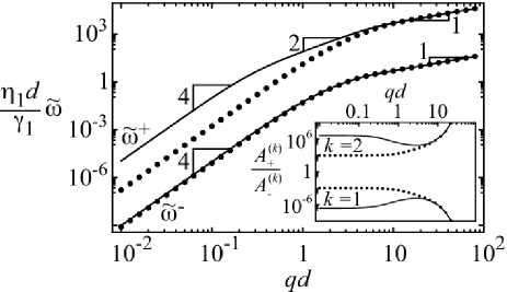
Figure 5: Dimensionless decay rates $\eta_{1}d\tilde{\omega}^{\pm}/\gamma_{1}$ and amplitude ratios $A_{+}^{(k)}/A_{+}^{(k)}$ (inset) as a function of $qd$ for a double layer system with a buried Newtonian PBrS layer and an upper Newtonian PS layer, using the parameter values given in Table 1. The solid (dotted) lines are for a system with a small (large) liquid/liquid slip length, $\lambda=0.01d$ ($\lambda=10d$).

In the case that both layers can be described as Newtonian fluids with viscosities $\eta_{1}(\omega)=\eta_{1}$ and $\eta_{2}(\omega)=\eta_{2}$, it is clear from Eq. (50) that $\det\bm{\Sigma}$ is a simple quadratic function of $\omega$. Thus, there are two normal mode decay rates, as expected from the arguments given in Appendix C. Specifically, the roots of Eq. (50) are given by

$$\tilde{\omega}^{\pm}(q)= \frac{q^{2}}{2\Phi}\Bigg{[}\gamma_{1}s_{22}+\gamma_{2}s_{11}\Bigg{.}$$ (53)

$$\Bigg{.}\pm\sqrt{\left(\gamma_{1}s_{22}+\gamma_{2}s_{11}\right)^{2}-4\gamma_{1}\gamma_{2}\Phi\Delta}\Bigg{]}$$

where $\tilde{\omega}^{\pm}\equiv i\omega^{\pm}$. The values of the fast mode $\tilde{\omega}^{+}$ and the slow mode $\tilde{\omega}^{-}$ for parameters consistent with a PBrS buried fluid and a PS upper fluid (see Table 1) are plotted in Fig. 5. The $\tilde{\omega}^{+}$, $\tilde{\omega}^{-}$ modes correspond to nearly in phase and out of phase undulations of the two surfaces, respectively.

Using Eqs. (IV)–(45), one can show that both normal mode decay rates exhibit the same asymptotic scaling behavior observed for the single viscous layer discussed above. When the slip length is small, $\lambda\ll d$,

$$\tilde{\omega}^{+}(q)= \begin{cases}\frac{\gamma_{2}q^{4}d_{2}^{3}}{3\eta_{2}}&qd\ll 1\\ \frac{\gamma_{2}|q|}{2\eta_{2}}&qd\gg 1\\ \end{cases},$$ (54)

$$\tilde{\omega}^{-}(q)= \begin{cases}\frac{\gamma_{1}q^{4}d_{1}^{3}}{3\eta_{1}}&qd\ll 1\\ \frac{\gamma_{1}|q|}{2\eta_{1}}&qd\gg 1\\ \end{cases}.$$ (55)

A large slip length at the fluid fluid interface (i.e. $\lambda\gg d$) produces an intermediate scaling regime in $\tilde{\omega}^{+}$,

$$\tilde{\omega}^{+}(q)=\begin{cases}\frac{\gamma_{2}q^{4}d_{2}^{2}\lambda}{\eta_{2}}&qd\ll 1,\,q^{2}d\lambda\ll 1\\ \frac{\gamma_{2}q^{2}d_{2}}{4\eta_{2}}&qd\ll 1,q^{2}d\lambda\gg 1\\ \frac{\gamma_{2}|q|}{2\eta_{2}}&qd\gg 1\end{cases}.$$ (56)

However, the value of $\tilde{\omega}^{-}$ is unaffected by the presence of a large slip length when $\eta_{1}\gg\eta_{2}$. Thus, we can see that, like the single layer case, a double layer of Newtonian fluids does not exhibit a $q$-independent decay rate, even in the presence of liquid-liquid slip.

Examining the normal mode amplitude ratio as a function of wave number, shown in the inset of Fig. 5, we see that at the upper surface the fast mode amplitude always dominates, while at the buried interface the slow mode always dominates. Thus, the decay of the height-height correlation functions, which are given by Eq. (IV), are essentially of the form of a single exponential decay, $S_{1}(q,t)\sim e^{-\tilde{\omega}^{-}t}$ and $S_{2}(q,t)\sim e^{-\tilde{\omega}^{+}t}$. The large size of the amplitude ratios at the two surfaces is due primarily to the large viscosity difference between the two layers. If we were to consider a two layer system having similar viscosities and similar interfacial tensions at the two surfaces, we would find amplitude ratios at the two surfaces of order unity. Of course, the rates themselves would be approximately equal as well in this limit.

IV.2 One Maxwell Fluid, One Newtonian Fluid

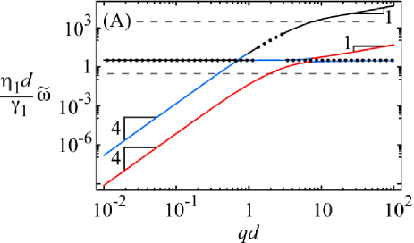
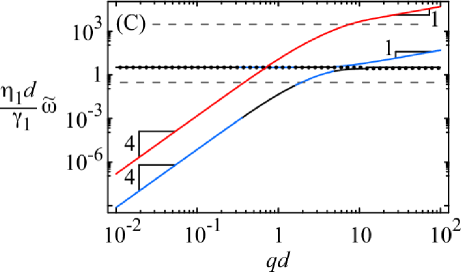
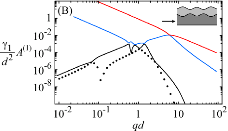
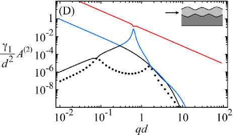
Figure 6: (color online) Dimensionless decay rates $\eta_{1}d\tilde{\omega}^{\pm}/\gamma_{1}$ (A, C) and amplitudes $\gamma_{1}A/d^{2}$ at the buried (B) and upper (D) interfaces, as a function of $qd$ for a double layer system with a buried Maxwell PBrS layer and an upper Newtonian PS layer in the absence of slip, using the parameter values given in Table 1. (A, C) The rates shown in these two figures are identical, except that the line styles in Fig. A correspond to those in Fig. B, while the line styles in Fig. C correspond to those in Fig. D. The dashed lines indicate the approximate window of decay rates that can be measured in the experiments, $10^{-3}s^{-1}<\tilde{\omega}<10s^{-1}$. (B, D) The amplitudes in these figures are indicated by dotted, black, blue, and red lines, in order of increasing amplitude.

When one of the fluids in the double layer is viscoelastic, we expect to find additional decay rates, as we found for the single viscoelastic layer. Here, we focus on the case of a buried viscoelastic fluid. It is known from the single layer experiments that PS fluid layers – the upper fluid in the double layer experiments – are well described by a purely viscous Newtonian fluid model kim:03 . On the other hand, we expect that the PBrS layer to have longer stress relaxation times. We model this viscoelastic layer using the Maxwell model, so that $\eta_{1}(\omega)$ is of the form of Eq. (23). This approach introduces two unknown rheological parameters for the material (namely, $E$ and $\tau$), which we discuss more fully below. For simplicity, we analyze this system with stick boundary conditions at all interfaces, i.e. $\lambda=0$.

From examining the zeros of Eq. (50) we find four separate decay rates for this dynamical system, in agreement with the arguments given in Appendix C. These decay rates for a double layer system with a buried PBrS layer and an upper PS layer are shown in Figs. 6A and  6C, using the parameters given in Table 1 (these two plots are identical, except that the line styles in each are chosen to correspond to Figs. 6B and  6D, respectively; we explain this in more detail below). The behavior of the decay rates is qualitatively similar to the single layer viscoelastic case. In particular, each rate has two major scaling regions: a $q$-dependent region, where the decay rate scales like the corresponding one in the Newtonian fluids case (i.e. $\sim q^{4}$ for small $qd$ or $\sim q$ for large $qd$), and a $q$-independent region. In the single layer case, however, the crossover between these two regions is abrupt and occurs at $qd\sim{\mathcal{O}}(1)$. This is not the case for the double layer system; indeed, one decay rate is essentially constant over the entire range of wave numbers shown in Fig. 6, with its $q$-dependent regime not appearing until higher wave numbers (data not shown).

In principle, all four decay rates shown in Fig. 6 contribute to the height-height correlation functions at both the upper and buried interface. As in the single layer case, though, the amplitudes corresponding to each decay rate are important in determining which rates can be observed experimentally in these correlation functions. Figs. 6B and  6D show the amplitudes for each decay rate at the buried and upper interfaces, respectively. The decay rates shown in Figs. 6A and 6C are plotted using the same line style (dotted, black, blue, and red) as their corresponding amplitude at the buried and upper interfaces, respectively. In these two figures we represent the experimentally accessible range of timescales by the region between the two grey dashed lines. From examining Figs. 6B and 6D it is clear that the ratios of the various amplitudes vary by many orders of magnitude over the experimentally accessible wave number range. Also, the dominant amplitude at both interfaces is always $q$-dependent, as was seen in the single layer case.

We consider first the dynamics of buried interface shown in Figs. 6A and 6B. If we focus on the wave number regime accessible in the experiments of Lal et al., $0.8\lesssim qd\lesssim 2$, we see that the slow, $q$-dependent rate, which has the largest amplitude at the buried interface, is too slow to be detected experimentally. The other decay rates all have amplitudes of approximately the same magnitude in this region. Thus, it appears that the buried layer dynamics should, in fact, be best described by a height autocorrelation function having multiple exponential decays. The data of Lal et. al, however, was consistent with single exponential decays at this interface. This could be due to the fact that decay rates do not differ substantially in this region (see the blue, black, and dotted curves in Fig. 6A), thus rendering it difficult to observe the multi-exponential decay profiles. We do predict, however, that the $q$-independent decay rate should be observable at the buried layer, in agreement with the experimental data.

We now turn to the dynamics of the free surface shown in Figs. 6C and 6D. We see that for wave numbers $qd\simeq 0.7$, it should be possible to observe a double exponential decay, since the amplitudes of the dominant, $q$-dependent decay rate (red line) and subdominant $q$-independent rate (blue line) are approximately equal, as shown in Fig. 6D. Furthermore, we can see from Fig. 6C that the $q$-dependent rate is slower than the $q$-independent rate in the experimental range of wave numbers, $0.8\lesssim qd\lesssim 2$. The experiments do indeed observe a double exponential decay with a faster $q$-dependent rate and a slower $q$-independent rate; however, the amplitude of the $q$-independent decay is larger than that of the $q$-dependent decay in the experiments, whereas the opposite is true for our theoretical predictions.

We suspect that pursuing more detailed numerical fits of the theory to the current experiments is unproductive due primarily to the inadequacies of the Maxwell model. In particular, a more realistic description of the stress relaxation in the PBrS layer will allow for a spectrum of relaxation times, leading to a band of decay rates at a given wave number. As is clear from Figs. 6C and D, the amplitudes of the decay rates are highly nonlinear, and thus are sensitive to the details of the viscoelastic model used for the fluid. As the theory currently stands, it appears to be fortuitous that one may observe the double exponential decay at the free surface, since amplitude ratio between the two dominant modes (red and blue lines) in this figure have an extremely narrow maximum at $qd\approx 0.7$. We expect, however, that a broadening of the relaxation time spectrum in the material will increase the width of the features in Fig. 6D, making the observation of the multiple exponential decay in the data much more plausible. It is important to note that the use of a more realistic viscoelastic model for the buried fluid should not affect the existence of the $q$-independent decay rates themselves. Indeed, the scaling arguments given in section II show that the presence of the $q$-independent decay rate is a robust feature of the elastic response of the fluid. Thus, a more realistic model for the buried fluid should be able to account for the discrepancies between our theory and the experimental results of Lal et al.

Finally, we note that when the upper fluid is a Maxwell fluid and the lower fluid is a Newtonian fluid, an additional decay rate appears, in agreement with the arguments given in Appendix C. Although four of the rates behave in a manner similar to that of the four decay rates for a buried Maxwell fluid – with each rate displaying one region of $q$-independent behavior and another region of $q$-dependent, Newtonian-like behavior – the fifth rate is essentially constant over the wave numbers of interest. Furthermore, we find that at certain wave numbers the amplitude of one of the $q$-independent decay rates can actually be as large as the largest $q$-dependent amplitudes in the height-height correlation functions, at both the buried and upper interfaces (data not shown). Thus, our analysis suggests that detecting the $q$-independent rates may be even easier when the upper fluid is viscoelastic. It is important to repeat, however, that we do not suspect that it is a viscoelastic response of the upper PS layer that is leading to the $q$-independent decay rates seen in the experiments, since the purely viscous model fits the single layer PS data well kim:03 .

V Conclusion

In this article we have examined in detail the overdamped dynamics of purely viscous and viscoelastic supported films, taking the effects of both liquid/substrate and liquid/liquid slip into account. These calculations show that a simple approach to understanding the appearance of wave number independent decay rates in the height autocorrelation function $S(q,t)$ in both single and double layer films is found by allowing for a viscoelastic response of the material. Simple scaling arguments show that a viscoelastic material will exhibit such dynamics over some finite wave number range. The more detailed continuum mechanics calculations based on the Maxwell fluid model presented above show that this wave number independent scaling regime is experimentally accessible, at least for a viscoelastic material with the appropriate values of the plateau modulus $E$ and the stress relaxation time $\tau$.

More generally, the appearance of a $q$-independent relaxation rate in $S(q,t)$ appears to be a signal of a viscoelastic response of the supported polymer film on the time scales probed by the measurement. The observed decay time is strongly controlled by the longest stress relaxation time in the material, and thus may serve as an important measure of the rheological properties of such thin supported films. In the numerical results that we presented our choice of the stress relaxation time $\tau$ is constrained by the value of the $q$-independent decay time measured in the experiments, which is of the order of $100$s. In order to fit the data, we had to take $\tau$ to be of this same order, which is almost two orders of magnitude larger longer than might be expected for PS at the reported molecular weight pedersen:99 . We suggest that discrepancy may be attributed to two factors. First, the bromination of the PS changes the microscopic dynamics of dynamics of the polymer. Second, the narrow thickness of the PBrS layer (the layer is about three radii of gyration of the chain in $\theta$-conditions) adds further constraints to the chain dynamics leading to a longer stress relaxation time.

Given a determination of $\tau$, we found that our choice of the plateau modulus was not as precisely constrained by the data. If we choose $E\tau/\eta_{1}\gg 1$, the value of the $q$-independent decay time is decreased below $\tau$. Since the value of $\tau$ needed to fit the data is already anomalously large, we wish to choose the smallest possible value of $\tau$: this restricts us to the region $E\tau/\eta_{1}\ll 1$. As long as we choose a value of $E$ within this region, though, the value of the $q$-independent decay rate is unaffected by it. Rather, the principal effect of varying the plateau modulus is to shift the various amplitude ratios of the multiple decay rates, in particular the wave numbers at which these ratios approach unity.

This points out two more general results. The first is that the appearance of multiple exponential decay rates of the height autocorrelation function $S(q,t)$ for a single layer system is a generic feature of our viscoelastic model. In a two-layer system, even purely viscous fluids admit a double exponential decay. If either of the layers is viscoelastic, then this double decay becomes a more complicated multiple decay as discussed above. Based on these calculations we suspect that the observation of multiple exponential decays of $S(q,t)$ in a single layer system may be taken as evidence of the viscoelasticity of the supported film. Secondly, our calculations show that observable multiple exponential decays depend on amplitude ratios that are in turn controlled by the plateau modulus of the material. These ratios can vary by many orders of magnitude with the plateau modulus and wave number. The observation of multiple exponential decays requires the ratio of the two largest amplitudes to be near unity; from our Maxwell-model based calculations such occurrences occupy a small part of the phase space spanned by wave number and plateau modulus. While we expect that a broader spectrum of stress relaxation times in the material will enlarge the region of phase space over which these multiple exponential decays can be seen, such multiple exponential decays may not be a generically observable feature of viscoelastic supported films. When such multiple exponential decays are observed, however, they should provide a sensitive window onto the plateau modulus of the material and thus measure the entanglement length in the layer.

Finally, we point out that these calculations do not in general exclude other potential mechanisms as the underlying cause of the dynamics as observed by XPCS. They do show, however, that these data are not consistent with the dynamics of two immiscible Newtonian fluids either with stick or slip boundary conditions at their boundaries. Moreover, one can show that postulating more complex surface energy functionals – including, for example, an interfacial bending modulus – will only lead to relaxation rates of $S(q,t)$ that are even more strongly dependent on the wave number, which would be inconsistent with the data. Therefore, such considerations can also be excluded. It appears that most simple way to account for the data is to postulate a viscoelastic response of the supported film with a stress relaxation time on the order of the observed decay rate of the height autocorrelation function.

A more detailed analysis of the interfacial dynamics of complex fluids via XPCS holds the promise of probing molecular motion in confined geometries that may be interpreted with the aid of the continuum modeling presented in this article. If our calculations are to serve in this manner, however, they must first be tested further by experiment on rheologically well-characterized materials of thickness large enough to discount the effects of molecular confinement.

Appendix A Solution of the Time-dependent Stokes Equation

For a low Reynolds number fluid whose velocity and pressure are of the form of Eq. (7), the time-dependent Stokes equation is given by

$$i\omega\rho\,{\bf v}(q,z,\omega)e^{iqx}= -\eta(\omega){\bf\nabla}^{2}\left[{\bf v}(q,z,\omega)e^{iqx}\right]$$ (57)

$$+{\bf\nabla}\left[P(q,z,\omega)e^{iqx}\right],$$

where $\rho$ is the fluid density and $\eta(\omega)$ is the frequency-dependent fluid viscosity. We also assume that the fluid is incompressible,

$${\bf\nabla}\cdot{\bf v}(x,t)=0\quad\Rightarrow\quad v_{x}(q,z,\omega)=\frac{i}{q}v_{z}^{\prime}(q,z,\omega),$$ (58)

where the prime indicates a derivative with respect to the $z$-coordinate. Using the identity ${\bf\nabla}\times\left[{\bf\nabla}\psi(x,z,t)\right]=0$ (for any scalar function $\psi$), we can take the curl of Eq. (57) to eliminate the pressure,

$$i\omega\rho\,\Omega_{y}(q,z,\omega)+\eta(\omega)\left[\partial_{z}^{2}-q^{2}\right]\Omega_{y}(q,z,\omega)=0,$$ (59)

where ${\bf\Omega}(x,z,t)\equiv{\bf\nabla}\times{\bf v}(x,z,t)=\Omega_{y}(x,z,t)\hat{y}$ is the fluid vorticity,

$$\Omega_{y}(q,z,\omega)=\frac{i}{q}v_{z}^{\prime\prime}(q,z,\omega)-iqv_{z}(q,z,\omega).$$ (60)

The solution to Eq. (59) can be written as

$$\Omega_{y}(q,z,\omega)=2qC_{1}\cosh(kz)+2qC_{2}\sinh(kz),$$ (61)

where $C_{1}$ and $C_{2}$ are constants of integration and $k\equiv\sqrt{q^{2}-\frac{i\omega\rho}{\eta(\omega)}}$. The $z$-component of the velocity obeys the differential equation Eq. (60), which has the solution

$$v_{z}(q,z,\omega)= C_{3}\cosh(qz)+C_{4}\sinh(qz)$$ (62)

$$+\int_{0}^{\infty}dz^{\prime}G(z-z^{\prime})\Omega_{y}(q,z^{\prime},\omega),$$

where the first two terms are the homogeneous solution to Eq. (60), and $G(z)$ is the Green’s function for the operator $i(\partial_{z}^{2}-q^{2})/q$, $G(z)=-i\sinh(qz)\theta(z)$, $\theta(z)$ being the Heaviside step function. Then the velocity is given by

$$v_{z}(q,z,\omega)=2C_{1}^{\prime}q^{2}\cosh(kz)+2C_{2}^{\prime}q^{2}\sinh(kz)$$ (63)

$$+\left(C_{3}-2C_{1}^{\prime}q^{2}\right)\cosh(qz)+\left(C_{4}-2C_{2}^{\prime}kq\right)\sinh(qz),$$

where $C_{j}^{\prime}\equiv C_{j}/(k^{2}-q^{2})$ for $j=1,2$.

The pressure can be obtained from the $x$-component of Eq. (57),

$$P(q,z,\omega)=\frac{\eta(\omega)}{q^{2}}\left[v_{z}^{\prime\prime\prime}(q,z,\omega)-k^{2}v_{z}^{\prime}(q,z,\omega)\right].$$ (64)

Note that the $z$-component of Eq. (57) is automatically satisfied by this pressure and the velocity field given by Eq. (63).

For overdamped fluids, where the inertial term in the time dependent Stokes equation – that is, the left-hand side of Eq. (57) – is negligible, we can set $\rho=0$, which causes $k\rightarrow q$. In this case, the velocity Eq. (63) is given by

$$v_{z}(q,z,\omega)= C_{3}\cosh(qz)+(C_{4}-C_{2})\sinh(qz)$$ (65)

$$+C_{1}qz\sinh(qz)+C_{2}qz\cosh(qz).$$

Appendix B The Fluctuation-Dissipation Theorem

The fluctuation-dissipation theorem relates correlations between the orthogonal dynamical variables describing some system at equilibrium to the response of these variables to external forces. For the single fluid layer system we consider in this paper, there is only one dynamical variable, the height of the fluid, $h(x,t)$. For the double layer system, there are two orthogonal dynamical variables, the normal modes amplitudes $h_{\alpha}(x,t)$, where $\alpha=\pm$. In both cases, the response function can be obtained from the normal stress boundary condition(s) at the fluid interface(s), which in the normal mode basis can be written in the form

$$\frac{h_{\alpha}(q,\omega)}{\xi_{\alpha}(q,\omega)}=f_{\alpha}(q,\omega).$$ (66)

The fluctuation-dissipation theorem relates the response function $\xi_{\alpha}(q,\omega)$ to the height-height correlation function

$$S_{\alpha}(q,t)\equiv \frac{\left(2\pi\right)^{3}}{k_{B}TL^{2}}\left<h_{\alpha}(q,t)h_{\alpha}^{*}(q,0)\right>$$ (67)

$$= \int_{-\infty}^{\infty}\frac{d\omega}{2\pi i\omega}e^{-i\omega t}\left[\xi_{\alpha}(q,\omega)-\xi_{\alpha}^{*}(-q,\omega)\right].$$

where $L^{2}\equiv\int d^{2}x$ and the star indicates complex conjugation.

The integral in Eq. (67) can be evaluated by contour integration using a semi-circular, negatively oriented contour $\mathcal{C}$ whose arc lies in the negative imaginary half-plane and whose diameter is the real axis. We can see from Eq. (66) that the frequencies for which $\xi^{-1}_{\alpha}(q,\omega)=0$ are precisely the normal mode frequencies $\omega_{n}$ [i.e. the frequencies that satisfy the normal stress boundary conditions Eq. (66) for $f_{\alpha}=0$]. Because the system is overdamped, these frequencies lie on the negative imaginary axis, within the contour $\mathcal{C}$; therefore, each normal mode frequency contributes a non-zero residue to the contour integral. Furthermore, it can be shown that, for all systems we consider in this paper, $\xi_{\alpha}^{*}(-q,\omega)=\xi_{\alpha}(q,-\omega)$. This implies that the second term in Eq. (67) has no poles inside the contour, nor does it contribute to the residues at the poles $\omega_{n}$. Assuming the poles at each $\omega_{n}$ are simple poles (which can be shown to be true in all cases), Eq. (67) becomes

$$S_{\alpha}(q,t)=-\sum_{\omega_{n}}\lim_{\omega\rightarrow\omega_{n}}\left[\left(\omega-\omega_{n}\right)\frac{\xi_{\alpha}(q,\omega)}{\omega}e^{-i\omega t}\right].$$ (68)

Appendix C Number of Normal Mode Decay Rates

The number of decay rates in a dynamical system is simply related to the number of independent degrees of freedom lubensky:book . It is therefore somewhat counterintuitive to observe two decay rates for capillary waves on a single supported viscoelastic layer and either four or five decay rates in the double layer system. It is perhaps most surprising to find the number of decay rates to change upon inverting the order of the layering of the two materials. In this appendix we explain this result in a simple way by considering the equations of motion in the time domain rather than in the frequency domain, as we have done throughout the rest of this article.

Let us first consider the single layer case. Here and throughout this appendix we suppress any wave number $q$ dependence for clarity. From the boundary condition Eq. (10) we see that $v_{z}(z,\omega)\propto-i\omega h(\omega)$. Using the boundary conditions Eqs. (8)-(11), we write the velocity in the form

$$v_{z}(z,\omega)=-i\omega h(\omega)\psi(z).$$ (69)

Taken in combination with the stress boundary condition Eq. (13) we find

$$\gamma q^{2}h(\omega)=-i\omega\eta(\omega)h(\omega)f(0),$$ (70)

where $f(z)\equiv 3\psi^{\prime}(z)-\psi^{\prime\prime\prime}(z)/q^{2}$.

For a Newtonian fluid, $\eta(\omega)=\eta$. Converting Eq. (70) back to the time domain we recover a first order differential equation for the decay of the surface height field:

$$\gamma q^{2}h(t)=\eta f(0)\dot{h}(t).$$ (71)

Thus, we expect only one decay rate at a given wave number for capillary waves on a single supported Newtonian fluid.

For the single supported Maxwell fluid the situation is more complicated. Now the viscosity is a complex frequency dependent function, which is given by Eq. (23). As a result, conversion of Eq. (70) into the time domain yields an integro-differential equation:

$$\frac{\gamma q^{2}}{f(0)}h(t)=\eta_{0}\dot{h}(t)-\frac{E_{0}}{\tau}\int_{-\infty}^{t}\!\!\!\!dt^{\prime}h(t^{\prime})e^{-\frac{t-t^{\prime}}{\tau}}.$$ (72)

The time evolution of the surface height now depends on the entire deformation history of the surface convoluted with an exponential memory kernel. The simple form of the memory kernel is an artifact of the simplicity of the Maxwell fluid, but the general structure of this equation of motion holds for any more complex model of viscoelasticity.

Taking a time derivative of Eq. (72) we may write a single, second order differential equation for the amplitude of the height field at wave vector ${\bf q}$:

$$\frac{\gamma q^{2}}{f(0)}\left[\tau\dot{h}(t)+h(t)\right]=\eta_{0}\left[\tau\ddot{h}(t)+\dot{h}(t)\right]-E_{0}h(t).$$ (73)

From this second order differential equation, which has two independent exponentially decaying solutions, we know to expect a double exponential decay for capillary waves on the supported Maxwell fluid.

We now consider the case of two fluid layers. As in the single layer case we can use the boundary conditions Eqs. (31)-(36) to write the fluid velocities in the form

$$v_{k,z}(z,\omega)=-i\omega\left[h_{1}(\omega)\psi_{k1}(z)+h_{2}(\omega)\psi_{k2}(z)\right],$$ (74)

with $k=1,2$ indexing the fluid layers. There remain three more boundary conditions. One enforces tangential stress continuity at the fluid/fluid interface; the other two set the difference in the normal stresses at both the fluid/fluid interface and the free surface in terms of their respective surface tensions. These conditions may be written as, respectively,

$$\eta_{1}(\omega)\sum_{k=1,2}g_{1k}(0)h_{k}(\omega)=\eta_{2}(\omega)\sum_{k=1,2}g_{2k}(0)h_{k}(\omega),$$ (75)

and

$$\gamma_{1}q^{2}h_{1}(\omega) =\sum_{j,k=1,2}(-1)^{j}i\omega h_{k}(\omega)\eta_{j}(\omega)f_{jk}(d_{2})$$ (76)

$$\gamma_{2}q^{2}h_{2}(\omega) =\sum_{k=1,2}i\omega\eta_{2}(\omega)g_{2k}(0)h_{k}(\omega),$$ (77)

where $f_{jk}(z)=3\psi_{jk}^{\prime}(z)-\psi_{jk}^{\prime\prime\prime}(z)/q^{2}$ and $g_{jk}(z)=q^{2}\psi_{jk}(z)+\psi_{jk}^{\prime\prime}(z)$. In a manner analogous to the one used above with the single layer problem, we can rewrite Eqs. (75)-(77) in the time domain. Note that the presence of the $i\omega$ factor in Eqs. (76) and (77) implies a time derivative.

When both fluids are Newtonian Eq. (75) involves no time derivatives, whereas both Eqs (76) and (77) are first order differential equations. Having a system of two first order differential equations, we expect two normal mode decay rates for a double layer of two immiscible Newtonian fluids.

If either the upper or buried fluid is a Maxwell fluid, then it clear from the arguments given in the single layer case that Eq. (75) becomes a first-order differential equation in the time domain, whereas Eq. (76) becomes a second order ODE. Eq. (77), on the other hand, depends only on the viscosity of the upper fluid, $\eta_{2}$, so it becomes a second order differential equation only when the upper fluid is a Maxwell fluid; otherwise, it is a first order differential equation. Therefore, if the upper layer is a Newtonian fluid we have a set of two first order differential equations and one second order differential equation; we expect there to be four decay rates in this case. If the upper fluid is a Maxwell fluid and the lower one is Newtonian, however, we now have a dynamical system described by one first order differential equation and two second order ones. In this case there will be five decay rates.

References

- (1) H.Lamb, Hydrodynamics Sixth Ed. (Dover, New York, 1932).
- (2) S. Hard and R.D. Neuman, J. Coll. Int. Sci. 115, 73 (1987).
- (3) C.J. Hughes and J.C. Earnshaw, Rev. Sci. Instr. 64, 2789 (1993).
- (4) L. Kramer, J. Chem. Phys. 55, 2097 (1971).
- (5) J.C. Earnshaw, Phys. Lett. A 92, 40 (1982).
- (6) Q.R. Huang and C.H. Wang, J. Chem. Phys. 105, 6546 (1996).
- (7) M.G. Munoz, M. Encinar, L.J. Bonales F. Ortega, R. Monroy and R. G. Rubio, J. Phys. Chem. B 109 4694 (2005).
- (8) H. Kim, H.N. Zhang, S. Narayanan, J. Wang, O. Prucker, J. Ruhe, and M.D. Foster, Polymer 46, 2331 (2005).
- (9) F. Monroy and D. Langevin, Phys. Rev. Lett. 81, 3167 (1998).
- (10) T.Thurn-Albrecht, W. Steffen, A. Patkowski, G. Meier, E.W. Fisher, G. Grübel, and D. L. Abernathy, Phys. Rev. Lett. 77, 5437 (1996).
- (11) C. Gutt, T. Ghaderi, V. Chamard, A. Madsen, T. Seydel, M. Tolan, M. Sprung, G. Grübel, and S.K. Sinha, Phys. Rev. Lett. 91, 076104 (2003).
- (12) J.L. Harden, H. Pleiner, and P.A. Pincus, J. Chem. Phys. 94, 5208 (1991).
- (13) J. Jäckle, J. Phys. Cond. Mat. 10, 7121 (1998).
- (14) M. Rauscher, A Münch, B. Wagner, and R. Blossey, Eur. Phys. J. E 17, 373 (2005).
- (15) V. Kumaran, J. Chem. Phys. 98, 3429 (1992).
- (16) J.L. Keddie, R.A.L. Jones, and R. Cory, Europhys. Lett. 27, 59 (1994).
- (17) R.G. de Gennes, Eur. Phys. J. E 2, 201 (2000).
- (18) J.D. McCoy and J.G. Curro, J. Chem. Phys. 116, 9154 (2002).
- (19) H. Kim, A. Rühm, L.B. Lurio, J.K. Basu, J. Lal, D. Lumma, S.G.J. Mochrie, and S.K. Sinha, Phys. Rev. Lett. 90, 068302 (2003).
- (20) X. Hu, Z. Jiang, S. Narayanan, X. Jiao, A. Sandy, S.K. Sinha, L.B. Lurio, and J. Lal, Phys. Rev. E 74, 010602 (R) (2006); Private Communication with J. Lal.
- (21) L.D. Landau and E.M. Lifshitz, Fluid Mechanics Second Edition (Elsevier, Amsterdam, 2004).
- (22) L.D. Landau and E.M. Lifshitz, Theory of Elasticity 3rd Ed (Pergamon Press Amsterdam, 1986).
- (23) J. S. Pedersen and P. Schurtenberger, Europhys. Lett. 45, 666 (1999).
- (24) P.M. Chaikin and T.C. Lubensky, Principles of Condensed Matter Physics (Cambridge University Press, Cambridge, 2000).