Kondo Effects in Carbon Nanotubes: From SU(4) to SU(2) symmetry

Abstract

We study the Kondo effect in a single-electron transistor device realized in a single-wall carbon nanotube. The $K$-$K^{\prime}$ double orbital degeneracy of a nanotube, which originates from the peculiar two-dimensional band structure of graphene, plays the role of a pseudo-spin. Screening of this pseudo-spin, together with the real spin, can result in an SU(4) Kondo effect at low temperatures. For such an exotic Kondo effect to arise, it is crucial that this orbital quantum number is conserved during tunneling. Experimentally, this conservation is not obvious and some mixing in the orbital channel may occur. Here we investigate in detail the role of mixing and asymmetry in the tunneling coupling and analyze how different Kondo effects, from the SU(4) symmetry to a two-level SU(2) symmetry, emerge depending on the mixing and/or asymmetry. We use four different theoretical approaches to address both the linear and non-linear conductance for different values of the external magnetic field. Our results point out clearly the experimental conditions to observe exclusively SU(4) Kondo physics. Although we focus on nanotube quantum dots, our results also apply to vertical quantum dots. We also mention that a finite amount of orbital mixing corresponds, in the pseudospin language, to having non-collinear leads with respect to the orbital ”magnetization” axis which defines the two pseudospin orientations in the nanotube quantum dot. In this sense, some of our results are also relevant to the problem of a Kondo quantum dot coupled to non-collinear ferromagnetic leads.

I Introduction

The first observations of Kondo effect in semiconductor quantum dots (QDs) Gold98 ; Cron98 ; Stutt98 have spurred a great deal of experimental and theoretical activity during the last few years. Since these experimental breakthroughs, remarkable achievements have been reported, including the observation of the unitary limit,Wiel00 the singlet-triplet Kondo effect, Sasaki00a Kondo effect in molecular conductors molecule , and the Kondo effect in QDs connected to ferromagnetic Pasupathy04a and superconducting reservoirs, Buitelaar02a just to mention a few.

Recently, Jarillo-Herrero et al. reported perhaps the most sophisticated example, namely the observation of an orbital Kondo effect in a carbon nanotube (CNT) quantum dot (QD).Jarillo-Herrero05a In these experiments it was shown that the delocalized electrons of the reservoirs can screen both the orbital pseudospin degrees of freedom in the CNT QD (the $K$-K^′ double orbital degeneracy of the two-dimensional band structure of graphene) and the usual spin degrees of freedom, resulting in an SU(4) Kondo effect at low temperatures. In a recent letter, ChoiMS05z we showed that quantum fluctuations between the orbital and spin degrees of freedom may indeed dominate transport at low temperatures and lead to this highly symmetric SU(4) Kondo effect. More recently, Sakano and KawakamiSakano06a have studied, using the Bethe ansatz method at zero temperature and the non-crossing approximation at finite temperatures, the more general case where the quantum numbers of $N$ degenerate orbital levels are conserved, and found new interesting features of the SU($2N$)-symmetric Kondo effect. Importantly, this is true provided that both the orbital and spin indices are conserved during tunneling. This poses an interesting question about the nature of the nanotube-lead contact because, in principle, there is no special reason why the orbital degrees of freedom in the CNT should be conserved during tunneling.

As mentioned, this orbital pseudospin originates from the peculiar electronic structure of the nanotube (NT). Jarillo-Herrero05a ; Minot04a ; Cao04a The electronic states of a NT form one-dimensional electron and hole sub-bands as a result of the quantization of the electron wavenumber $k_{\perp}$ perpendicular to the NT axis, which arises when graphene is wrapped into a cylinder to create a NT. By symmetry, for a given sub-band at $k_{\perp}=k_{0}$ there is a second degenerate sub-band at $k_{\perp}=-k_{0}$. Semiclassically, this orbital degeneracy corresponds to the clockwise ($\circlearrowright$) or counterclockwise ($\circlearrowleft$) symmetry of the wrapping modes. A plausible explanation of why this degree of freedom is preserved during tunneling could be that the QD is likely coupled to NT electrodes (the metal electrodes are deposited on top of the NT so maybe the electrons tunneling out of the QD enter the NT section underneath the contacts) but this issue clearly deserves a thorough microscopic analysis about the nature of the contacts. The conservation of the orbital quantum number seems more likely in the vertical quantum dots (VQD),Sasaki04a where the orbital quantum number is the magnetic quantum number of the angular momentum.

Here, we take a different route and, assuming some degree of mixing in the orbital channel, ask ourselves about the robustness of the SU(4) Kondo effect against asymmetry in the couplings and/or mixing.

The rest of the paper is organized as follows: In Section II we introduce the relevant model Hamiltonian and classify different schemes of the lead-dot coupling. These different coupling schemes result in different symmetries and hence affect significantly the underlying Kondo physics. These effects are analyzed in the subsequent sections. Section III presents the analysis with two renormalization group (RG) approaches. In Sec. IV two slave-boson approaches complement the previous results. Finally, Sec. V concludes the paper.

II Model

II.1 Nearly Degenerate Localized Orbitals

We consider a QD with two (nearly) degenerate localized orbitals which is coupled to reservoirs. As we mentioned before, we have in mind the experimental setup of Ref. Jarillo-Herrero05a, where a highly symmetric Kondo effect was demonstrated in a CNT QD. However, our description could well apply to vertical quantum dot (VQD),Sasaki04a where the orbitals correspond to two degenerate Fock-Darwin states with different values of the angular momentum quantum number. Hereafter we denote this orbital quantum number by $m=1,2$. The dot is then described by the Hamiltonian

$$H_{D}=\sum_{m=1,2}\sum_{\sigma=\uparrow,\downarrow}\epsilon_{m\sigma}d_{m\sigma}^{\dagger}d_{m\sigma}\\ \mbox{}+\sum_{(m,\sigma)\neq(m^{\prime},\sigma^{\prime})}U_{mm^{\prime}}n_{m\sigma}n_{m^{\prime}\sigma^{\prime}}\,,$$ (1a)

where $$\epsilon_{m\sigma} m \sigma d_{m\sigma}^{\dagger} d_{m\sigma} n_{m\sigma}=d_{m\sigma}^{\dagger}d_{m\sigma} U_{mm} m=1,2 U_{12} \Delta_{\mathrm{orb}} \Delta_{Z} \epsilon_{m\sigma}$$ is the single-particle energy level of the localized state with orbital and spin , () the fermion creation (annihilation) operator of the state, the occupation number operator, () the intra-orbital Coulomb interaction, and the inter-orbital Coulomb interaction. The effect of the external magnetic field parallel to the symmetry axis of the system is to lift the orbital and spin degeneracy of the single-particle energy levels. We will denote them by and , respectively, so that the single-particle energy levels have the form

$$\epsilon_{m\sigma}=\epsilon_{0}+\Delta_{\mathrm{orb}}(\delta_{m,1}-\delta_{m,2})+(\Delta_{Z}/2)(\delta_{\sigma,\uparrow}-\delta_{\sigma,\downarrow})\,.$$ (1b)

The precise values of the Coulomb interactions $$U_{mm^{\prime}} E_{C}=e^{2}/2C C \sum_{m\sigma}\left\langle\textstyle n_{m\sigma}\right\rangle\approx 1 U_{mm^{\prime}}\sim E_{C}$$ depend on the details of the system, but should be of the order of the charging energy with being the total capacitance of the dot. In this work we focus on the regime where the system of the localized levels is occupied by a single electron (, quarter filling half-filling ) and the Coulomb interaction energy () is much bigger than other energy scales. In this regime the Hamiltonian in Eq. (1a) suffices to describe all relevant physics of our concern.

II.2 Coupling Schemes

Kondo physics arises as a result of the interplay between strong correlations in the dot and coupling of the localized electrons with the itinerant ones in conduction bands. Naturally, different Kondo effects are observed depending on the way the dot is coupled to the electrodes and whether or not the orbital quantum number $m$ is conserved. Nevertheless, it turns out highly non-trivial experimentally to distinguish those different Kondo effects. In subsequent sections we will consider different coupling schemes between the dot and the electrodes, show how different physics emerges, and propose how to distinguish them unambiguously in experiments.

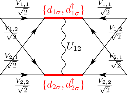
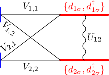
Figure 1: (color online) Schematic of a representative mesoscopic system in question. In (a) Each of the two leads, $L$ and $R$, has two conduction bands (or “modes”), $1$ and $2$. The model with two leads in (a) is equivalent in equilibrium to the model in (b) with only one lead. The operators $c_{k\mu\sigma}$ ($\mu=1,2$ and $\sigma=\uparrow,\downarrow$) are related to $a_{Lk\mu\sigma}$ and $a_{Rk\mu\sigma}$ by the canonical transformation in Eq. (4). The wiggly lines indicate the inter-orbital Coulomb interaction $U_{12}$ whereas the intra-orbital interaction $U_{mm}$ ($m=1,2$) is not shown.

The two leads $\alpha=L$ and $R$ are treated as non-interacting gases of fermions:

$$H_{\alpha}=\sum_{k}\sum_{\mu=1,2}\sum_{\sigma}\epsilon_{\alpha k\mu}\,a_{\alpha k\mu\sigma}^{\dagger}a_{\alpha k\mu\sigma}\,,$$ (1c)

where $\mu$ denotes channels in the leads. Without loss of generality, we assume that there are two distinguished (groups of) channels $\mu=1$ and $2$ in each lead. When the leads bears the same symmetry as the dot, this channel quantum number $\mu$ in the leads is identical to the orbital quantum number $m$ in the dot and will be preserved over the tunneling of electrons from the dot to leads and vice versa; see Fig. 1(a). Otherwise, the orbital channels become mixed. The most general situation is described by the tunneling Hamiltonian

$$H_{T}=\sum_{\alpha k\mu\sigma}\left(V_{\alpha k\mu m\sigma}a_{\alpha k\mu\sigma}^{\dagger}d_{m\sigma}+h.c.\right)$$ (1d)

and the total Hamiltonian is thus given by $H=H_{L}+H_{R}+H_{T}+H_{D}$ .

For the sake of simplicity, we assume identical electrodes ($\epsilon_{Lk\mu}=\epsilon_{Rk\mu}$) together with symmetric tunneling junctions ($V_{Lk\mu m\sigma}=V_{Rk\mu m\sigma}$), and ignore their $k$- and $\sigma$-dependence of the tunneling amplitudes. In this way, we consider a simplified model with $V_{\alpha k\mu m\sigma}=V_{\mu,m}/\sqrt{2}$ and define the widths

$$\Gamma_{m}\equiv\Gamma_{mm}\,,\quad\Gamma_{mm^{\prime}}=\pi\rho_{0}V_{m}^{*}V_{m^{\prime}}\,$$ (2)

with $V_{m}\equiv V_{m,m}$, where $\rho_{0}$ is the density of states (DOS) in the reservoirs. Then in equilibrium the Hamiltonian $H$ in Eq. (1) is equivalent to $H=H_{C}+H_{T}+H_{D}$ with

$$H_{C} =\sum_{k\mu\sigma}\varepsilon_{k\mu}c_{k\mu\sigma}^{\dagger}c_{k\mu\sigma}\,,$$ (3a)

$$H_{T} =\sum_{k\mu m\sigma}\left(V_{\mu,m}c_{k\mu\sigma}^{\dagger}d_{m\sigma}+h.c.\right)\,,$$ (3b)

where we have performed the canonical transformation

$$\begin{split}c_{k\mu\sigma}&=\frac{a_{Lk\mu\sigma}+a_{Rk\mu\sigma}}{\sqrt{2}}\,,\\ b_{k\mu\sigma}&=\frac{a_{Lk\mu\sigma}-a_{Rk\mu\sigma}}{\sqrt{2}}\,,\end{split}$$ (4)

and discarded the decoupled term $\epsilon_{k\mu}b_{k\mu\sigma}^{\dagger}b_{k\mu\sigma}$.

In the following sections we investigate the physics described by the Hamiltonian in Eq. (3) and, in particular, clarify the role of index conservation in the symmetry of the underlying Kondo regime at low temperatures. In order to carry out this analysis, we use four different approaches: the scaling theory (perturbative RG approach), the numerical renormalization group (NRG) method, the slave-boson mean-field theory (SBMFT), and the non-crossing approximation (NCA).

III Renormalization Group Approaches

The renormalization group (RG) theory provides a convenient and powerful method to study low-energy properties of strongly correlated electron systems. Here we take two RG approaches, the scaling theoryAnderson70a ; Haldane78a ; Haldane78b and the NRG method. Wilson75a ; Krishna-murthy80a ; Costi94a ; Hofstetter00a While the scaling theory is useful for qualitative understanding of the model, a more precise quantitative analysis requires the use of more sophisticated methods like the NRG method. This method is known to be one of the most accurate and powerful theoretical tools to study quantum impurity problems (see Appendix A).

III.1 SU(4) Kondo Effect

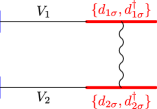
Figure 2: (color online) Schematics of the SU(4)-symmetric Anderson model.

We now turn to the case where tunneling processes conserve the orbital quantum number; see Fig. 2. In this case, the Hamiltonian reads

$$H=\sum_{\alpha=L,R}\sum_{m=1,2}\sum_{k\sigma}\varepsilon_{\alpha k}a_{\alpha km\sigma}^{\dagger}a_{\alpha km\sigma}\\ \mbox{}+\sum_{\alpha km\sigma}V_{m}\left(a_{\alpha km\sigma}^{\dagger}d_{m\sigma}+d_{m\sigma}^{\dagger}a_{\alpha km\sigma}\right)+H_{D}$$ (5)

or [see Eqs. (3a) and (3b)]

$$H=\sum_{km\sigma}\epsilon_{k}c_{k\sigma}^{\dagger}c_{km\sigma}\\ \mbox{}+\sum_{km\sigma}V_{m}\left(c_{km\sigma}^{\dagger}d_{m\sigma}+d_{m\sigma}^{\dagger}c_{km\sigma}\right)+H_{D}\,.$$ (6)

From the RG point of view, starting initially with nearly degenerate levels, all the localized levels are relevant for the spin and orbital fluctuations, and, as we shall see below, contribute to the Kondo effect. To investigate the low-energy properties of the orbital and spin fluctuations of the model, we perform the Schrieffer-Wolf (SW) transformation and obtain an effective Kondo-type Hamiltonian:

$$H=\sum_{km\sigma}\epsilon_{k}c_{km\sigma}^{\dagger}c_{km\sigma}+H_{\mathrm{eff}}^{\mathrm{SU(4)}}-\Delta_{Z}S^{z}-2\Delta_{\mathrm{orb}}T^{z}\\ \mbox{}-\frac{\left(\sqrt{J_{1}}-\sqrt{J_{2}}\right)^{2}}{2}(1+4\mathbf{s}\cdot\mathbf{S})(t^{x}T^{x}+t^{y}T^{y})\\ \mbox{}+(J_{1}-J_{2})(\mathbf{s}\cdot\mathbf{S})(t^{z}+T^{z})\,,$$ (7)

where

$$H_{\mathrm{eff}}^{\mathrm{SU(4)}}=\frac{J_{1}+J_{2}}{2}\left[\mathbf{s}\cdot\mathbf{S}+\mathbf{t}\cdot\mathbf{T}+4(\mathbf{s}\cdot\mathbf{S})(\mathbf{t}\cdot\mathbf{T})\right]\,$$ (8)

and the exchange coupling constants $J_{m}$ ($m=1,2$) are given by

$$J_{m}=V_{m}^{2}\left(\frac{1}{E_{+}}+\frac{1}{E_{-}}\right)\,.$$ (9)

We note that the Kondo-type effective Hamiltonian in Eq. (7) reduces to the SU(4)-symmetric Kondo model when $V_{1}=V_{2}$ and $\epsilon_{1\sigma}=\epsilon_{2\sigma}$. In this case, orbitals play exactly the same role as spins; the former are not distinguished from the latter.

Under the RG transformation reducing subsequently the conduction band width $D$ by $\delta{D}$, the Kondo-type effective Hamiltonian evolves into a generic form:

$$H_{\mathrm{eff}}=H_{\mathrm{leads}}-\Delta_{Z}S^{z}-2\Delta_{\mathrm{orb}}T^{z}\\ \mbox{}+2J_{1}(\mathbf{s}\cdot\mathbf{S})\left(\frac{1}{2}+t^{z}\right)\left(\frac{1}{2}+T^{z}\right)\\ \mbox{}+2J_{2}(\mathbf{s}\cdot\mathbf{S})\left(\frac{1}{2}-t^{z}\right)\left(\frac{1}{2}-T^{z}\right)\\ \mbox{}+\frac{1}{2}\left[J_{4}+4J_{3}(\mathbf{s}\cdot\mathbf{S})\right](t^{+}T^{-}+t^{-}T^{+})\\ \mbox{}+J_{5}t^{z}T^{z}\,.$$ (10)

The level splitting $\Delta_{\mathrm{orb}}$ and $\Delta_{Z}$ remain constant under the RG transformation:

$$\frac{d\Delta_{Z}}{d\ln D}=\frac{d\Delta_{\mathrm{orb}}}{d\ln D}=0\,.$$ (11)

The exchange coupling constants $J_{i}$ ($i=1,\cdots,5$) are initially given by Eq. (9) and

$$J_{3}=J_{4}=\sqrt{J_{1}J_{2}}\,,\quad J_{5}=\frac{1}{2}(J_{1}+J_{2})\,,$$ (12)

which, under the RG transformation, scale as

$$\frac{dJ_{1}}{\rho_{0}d\ln D} =-2J_{1}^{2}-J_{3}(J_{3}+J_{4})\,,$$ (13a)

$$\frac{dJ_{2}}{\rho_{0}d\ln D} =-2J_{2}^{2}-J_{3}(J_{3}+J_{4})\,,$$ (13b)

$$\frac{dJ_{3}}{\rho_{0}d\ln D} =-J_{3}(J_{1}+J_{2}+J_{5})-\frac{1}{2}J_{4}(J_{1}+J_{2})\,,$$ (13c)

$$\frac{dJ_{4}}{\rho_{0}d\ln D} =-\frac{3}{2}J_{3}(J_{1}+J_{2})-J_{4}J_{5}\,,$$ (13d)

$$\frac{dJ_{5}}{\rho_{0}d\ln D} =-3J_{3}^{2}-J_{4}^{2}\,$$ (13e)

for $D\gg\Delta_{\mathrm{orb}}\geq\Delta_{Z}$. For $D\ll\Delta_{\mathrm{orb}}$, it is clear from Eq. (10) that the orbital fluctuations are frozen and only $J_{1}$ is relevant, which scales as

$$\frac{dJ_{1}}{\rho_{0}d\ln D}=-2J_{1}^{2}.$$ (14)

It implies that we recover the single-level Anderson model for $D\ll\Delta_{\mathrm{orb}}$. Therefore in the remainder of this section, we will focus on the case $D\gg\Delta_{\mathrm{orb}}$.

It is convenient to define the reduced variables $j_{i}\equiv J_{i}/J_{1}$ ($i=2,\cdots,5$) and rewrite the RG equations (13) as

$$\frac{dj_{2}}{dx} =-j_{2}+\frac{2j_{2}^{2}+j_{3}(j_{3}+j_{4})}{2+j_{3}(j_{3}+j_{4})},$$ (15a)

$$\frac{dj_{3}}{dx} =-j_{3}+\frac{j_{3}(1+j_{2}+j_{5})+(j_{4}/2)(1+j_{2})}{2+j_{3}(j_{3}+j_{4})},$$ (15b)

$$\frac{dj_{4}}{dx} =-j_{4}+\frac{(3j_{3}/2)(1+j_{2})+j_{4}j_{5}}{2+j_{3}(j_{3}+j_{4})},$$ (15c)

$$\frac{dj_{5}}{dx} =-j_{5}+\frac{3j_{3}^{2}+j_{4}^{2}}{2+j_{3}(j_{3}+j_{4})}\,$$ (15d)

with $x=\ln(\rho_{0}J_{1})$, while $J_{1}$ obeys the scaling equation

$$\frac{1}{(\rho_{0}J_{1})^{2}}\frac{d(\rho_{0}J_{1})}{d\ln D}=-2-j_{3}(j_{3}+j_{4})\,.$$ (16)

The RG equations (15) have two fixed points: one describing the SU(4) Kondo physics

$$j_{2}=j_{3}=j_{4}=j_{5}=1$$ (17)

and the other describing the usual SU(2) Kondo physics

$$j_{2}=j_{3}=j_{4}=j_{5}=0\,,$$ (18)

both with $J_{1}=\infty$ as indicated in Fig. 3. Linearizing the RG equations (15) around the fixed points, one can easily show that both the SU(2) and SU(4) Kondo fixed points are stable (there is one marginal parameter at the SU(4) fixed point). However, as indicated as a dashed semicircle in Fig. 3(b), the radius of convergence is finite while the fixed point itself is located at infinity. This implies that in priciple, the SU(4) Kondo fixed point cannot be reached for arbitrarily small values of $1-\Gamma_{2}/\Gamma_{1}$. However, as illustrated in Fig. 3(a), in the region of physical interest for sufficiently small values of $1-\Gamma_{2}/\Gamma_{1}$, the scaling behavior is essentially governed by the SU(4) Kondo fixed point (see also Fig. 5). More importantly, for sufficiently small values of $1-\Gamma_{2}/\Gamma_{1}$, the SU(2) fixed point governs the physics only at extremely low energies. This suggests that the SU(4) Kondo signature can be observed exclusively at relatively higher energy scales (of the order of the Kondo temperature), as in the experiment reported recently. Jarillo-Herrero05a

Figure 3: (color online) RG flows for different values of $\Gamma_{2}/\Gamma_{1}$ with $\Gamma_{1}$ fixed.

At $B_{\parallel}=0$ and $\Gamma_{1}=\Gamma_{2}\equiv\Gamma_{0}$, the RG equations (13) reduce to a single equation

$$\frac{dJ_{1}}{\rho_{0}d\ln D}=-4J_{1}^{2}.$$ (19)

Comparing this with the corresponding one in Eq. (14) for the usual single-level Anderson model, we note that the Kondo temperature is enhanced exponentially:

$$T_{K}^{SU(4)}\sim\exp(-1/4\rho_{0}J_{1})\,$$ (20)

with respect to the SU(2) Kondo temperature

$$T_{K}^{SU(2)}\sim\exp(-1/2\rho_{0}J_{1})\,.$$ (21)

The perturbative RG analysis discussed above, whose validity is guaranteed only for $\rho_{0}J_{i}\ll 1$, turns out to be qualitatively correct in a wide region of the parameter space and provides a clear interpretation of the model. To confirm the perturbative RG analysis and make quantitative analysis, we use the NRG method (described in Appendix A), the results of which are summarized in Figs. 4–5. There the total spectral density

$$A_{d}(E)=\sum_{\sigma}\sum_{mm^{\prime}}\pi\Gamma_{mm^{\prime}}A_{m^{\prime}m;\sigma}(E)\,,$$ (22)

which provides direct information on the linear conductance Meir92a , is plotted.

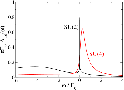
Figure 4: Comparison of the SU(2) and SU(4) Kondo model.

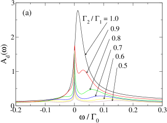
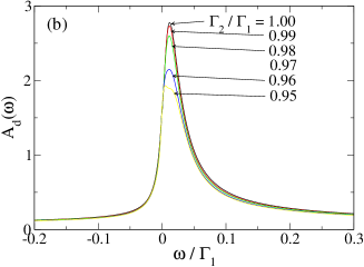
Figure 5: (color online) NRG results of the total spectral density $A_{d}(E)$ for different values of coupling asymmetry $\Gamma_{2}/\Gamma_{1}$. The parameter values are: $\epsilon_{0}=-0.8D$, $\Gamma_{1}=0.1D$, $U_{mm^{\prime}}=8D$, and $\Delta_{\mathrm{orb}}=\Delta_{Z}=0$.

The spectral density shows a peak near the Fermi energy, corresponding to the formation of the SU(4) Kondo state (see Fig. 4). The peak width, which is much broader than that for the SU(2) Kondo model (represented by the dotted line), demonstrates the exponential enhancement of the Kondo temperature mentioned above. Another remarkable effect is that the SU(4) Kondo peak shifts away from $\omega=E_{F}=0$ and is pinned at $\omega\approx T_{K}^{\mathrm{SU(4)}}$. This can be understood from the Friedel sum rule, Langreth66a which in this case gives $\delta=\pi/4$ for the scattering phase shift at $E_{F}$. Accordingly, the linear conductance at zero temperature is given by $\mathcal{G}_{0}=4(e^{2}/h)\sin^{2}\delta=2e^{2}/h$. It is interesting to recall that the Friedel sum rule gives the same linear conductance also for the two-level SU(2) Kondo model. Thus, neither the enhancement of the Kondo temperature nor the linear conductance can distinguish between the SU(4) and the two-level SU(2) Kondo effects. This can be achieved only by studying the influence of a parallel magnetic field in the nonlinear conductance, as shown in Ref. Jarillo-Herrero05a,

III.2 Effects of Mixing of Orbital Quantum Numbers

Figure 6: (color online) Model with finite mixing between orbital quantum numbers.

To examine the stability of the SU(4) Kondo phenomena against orbital mixing, we consider the model (see Fig. 6):

$$H=\sum_{k\sigma}\varepsilon_{k}c_{k\sigma}^{\dagger}c_{k\sigma}+\sum_{km\sigma}V_{0}\left(c_{km\sigma}^{\dagger}d_{m\sigma}+d_{m\sigma}^{\dagger}c_{km\sigma}\right)\\ \mbox{}+\sum_{km\sigma}V_{X}\left(c_{k\bar{m}\sigma}^{\dagger}d_{m\sigma}+d_{m\sigma}^{\dagger}c_{k\bar{m}\sigma}\right)+H_{D}\,,$$ (23)

where the indices imply $\bar{1}=2$ and $\bar{2}=1$ and $V_{0}\equiv V_{1,1}=V_{2,2}$ and $V_{X}\equiv V_{1,2}=V_{2,1}$.

If we rewrite the Hamiltonian in the form

$$H = \sum_{k\sigma}\varepsilon_{k}c_{k\sigma}^{\dagger}c_{k\sigma}+\sum_{km\sigma}\{V_{0}c_{km\sigma}^{\dagger}+V_{X}c_{k\bar{m}\sigma}^{\dagger}\}d_{m\sigma}$$ (24)

$$+ d_{m\sigma}^{\dagger}\{V_{0}c_{km\sigma}+V_{X}c_{k\bar{m}\sigma}\}+H_{D}\,,$$

it now becomes clear that, in the pseudospin language, a finite amount of orbital mixing corresponds to having non-collinear leads with respect to the orbital “magnetization” axis which defines the pseudospin orientations $m=1$ and $m=2$ in the dot. In other words, each confined electron (with defined pseudospin) couples to a linear combination of pseudospins and, as a result, becomes rotated in the pseudospin space by the angle defined by $\tan\phi=V_{X}/V_{0}$. Note that for the maximal mixing $V_{X}=V_{0}$, the tunneling electrons lose completely information about their pseudospin orientation. In this limit, one recovers the spin Kondo physics [with SU(2) symmetry] of a two-level Anderson model [see the next subsection and Eq. (36)]. For zero mixing ($V_{X}=0$), the model reduces to the SU(4)-symmetric model of Eq. (6) (with tunneling amplitudes which do not depend on the orbital index).

After the RG transformation of the Anderson-type model in Eq. (23) until the single-particle energy levels are comparable with the conduction band width (when the charge fluctuations are suppressed), the SW transformation gives

$$H_{\mathrm{eff}}=\left(1-\frac{J_{X}}{J_{0}}\right)H_{\mathrm{eff}}^{\mathrm{SU(4)}}+\frac{J_{X}}{J_{0}}H_{\mathrm{eff}}^{\mathrm{SU(2)}}\\ \mbox{}+J_{0}\sqrt{\frac{J_{X}}{J_{0}}}\left(1-\sqrt{\frac{J_{X}}{J_{0}}}\right)(1+4\mathbf{s}\cdot\mathbf{S})(t^{x}+T^{x})\\ \mbox{}+2J_{X}(t^{x}T^{x})\,,$$ (25)

where

$$H_{\mathrm{eff}}^{\mathrm{SU(4)}}=J_{0}\left[\mathbf{s}\cdot\mathbf{S}+\mathbf{t}\cdot\mathbf{T}+4(\mathbf{s}\cdot\mathbf{S})(\mathbf{t}\cdot\mathbf{T})\right]$$ (26)

corresponds to the SU(4) Kondo model and

$$H_{\mathrm{eff}}^{\mathrm{SU(2)}}=2J_{0}\mathbf{s}\cdot\mathbf{S}(1+2t^{x})(1+2T^{x})+J_{0}(t^{x}+T^{x})\,.$$ (27)

the SU(2) Kondo model. The exchange coupling constants $J_{0}$ and $J_{X}$, respectively, are given by

$$J_{0}=|V_{0}|^{2}\left(\frac{1}{E_{+}}+\frac{1}{E_{-}}\right)\,,\quad J_{X}=|V_{X}|^{2}\left(\frac{1}{E_{+}}+\frac{1}{E_{-}}\right)\,.$$ (28)

One can already grasp an idea about the effects of the mixing $J_{X}$ (i.e., $\Gamma_{X}$) of the orbital quantum numbers by considering the two limiting cases, $J_{X}=0$ (no mixing) and $J_{X}=J_{0}$ (maximal mixing), of the effective Hamiltonian (25). In the case of no mixing ($J_{X}=0$), the effective Hamiltonian (25) reduces to the SU(4)-symmetric Kondo model in Eq. (26), which has been already discussed in the previous section: The Kondo temperature is given by $T_{K}\sim D\exp(-1/4J_{0})$. When the mixing is maximal ($J_{X}=J_{0}$), on the other hand, the effective Hamiltonian becomes $H_{\mathrm{eff}}^{\mathrm{SU(2)}}$ in Eq. (27).

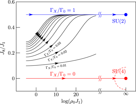
Figure 7: (color online) RG flows in case that there is a finite amount of mixing of the orbital quantum numbers.

Under the RG procedure, the effective Hamiltonian (25) transforms to the general form

$$H_{\mathrm{eff}}=J_{1}\mathbf{s}\cdot\mathbf{S}+\left[J_{3}(t^{z}T^{z})+4J_{2}(\mathbf{s}\cdot\mathbf{S})(t^{z}T^{z})\right]\\ \mbox{}\quad+\left[J_{4}(t^{x}T^{x}+t^{y}T^{y})+4J_{6}(\mathbf{s}\cdot\mathbf{S})(t^{x}T^{x}+t^{y}T^{y})\right]\\ \mbox{}\quad+\left[J_{5}(t^{x}T^{x}-t^{y}T^{y})+4J_{7}(\mathbf{s}\cdot\mathbf{S})(t^{x}T^{x}-t^{y}T^{y})\right]\\ \mbox{}\quad+\left[J_{9}+4J_{8}(\mathbf{s}\cdot\mathbf{S})(t^{x}+T^{x})\right]\,,$$ (29)

where the exchange coupling constants are initially given by

$$J_{1}=J_{0}+J_{X}\,,\quad J_{2}=J_{3}=J_{0}-J_{x}\,,\\ \mbox{}J_{4}=J_{6}=J_{0}\,,\quad J_{5}=J_{7}=J_{X}\,,\\ \mbox{}J_{9}=J_{8}=\sqrt{J_{0}J_{X}}\,.$$ (30)

Under the RG transformation, they scale as

$$\frac{dJ_{1}}{\rho_{0}d\ln D} =-J_{1}^{2}-J_{2}^{2}-2J_{6}^{2}-2J_{7}^{2}-8J_{8}^{2}\,,$$ (31a)

$$\frac{dJ_{2}}{\rho_{0}d\ln D} =-2J_{1}J_{2}-2J_{4}J_{6}+2J_{5}J_{7}\,,$$ (31b)

$$\frac{dJ_{3}}{\rho_{0}d\ln D} =-J_{4}^{2}+J_{5}^{2}-3J_{6}^{2}+3J_{7}^{2}\,,$$ (31c)

$$\frac{dJ_{4}}{\rho_{0}d\ln D} =-J_{3}J_{4}-3J_{2}J_{6}\,,$$ (31d)

$$\frac{dJ_{5}}{\rho_{0}d\ln D} =J_{3}J_{5}+3J_{2}J_{7}\,,$$ (31e)

$$\frac{dJ_{6}}{\rho_{0}d\ln D} =-J_{2}J_{4}-2J_{1}J_{6}-J_{3}J_{6}-4J_{8}^{2}\,,$$ (31f)

$$\frac{dJ_{7}}{\rho_{0}d\ln D} =J_{2}J_{5}-2J_{1}J_{7}+J_{3}J_{7}-4J_{8}^{2}\,,$$ (31g)

$$\frac{dJ_{8}}{\rho_{0}d\ln D} =-2J_{1}J_{8}-2J_{6}J_{8}-2J_{7}J_{8}\,,$$ (31h)

and

$$\frac{dJ_{9}}{d\ln D}=0\,.$$ (32)

As before [see Eq. (15)], it is convenient to work with the reduced coupling constants $j_{i}\equiv{}J_{i}/J_{1}$. In terms of these reduced constants, the RG equations read

$$\frac{dj_{2}}{dx} =-j_{2}+\frac{2j_{2}+2j_{4}j_{6}-2j_{5}j_{7}}{1+j_{2}^{2}+2j_{6}^{2}+2j_{7}^{2}+8j_{8}^{2}}\,,$$ (33a)

$$\frac{dj_{3}}{dx} =-j_{3}+\frac{j_{4}^{2}-j_{5}^{2}+3j_{6}^{2}-3j_{7}^{2}}{1+j_{2}^{2}+2j_{6}^{2}+2j_{7}^{2}+8j_{8}^{2}}\,,$$ (33b)

$$\frac{dj_{4}}{dx} =-j_{4}+\frac{j_{3}j_{4}+3j_{2}j_{6}}{1+j_{2}^{2}+2j_{6}^{2}+2j_{7}^{2}+8j_{8}^{2}}\,,$$ (33c)

$$\frac{dj_{5}}{dx} =-j_{5}-\frac{j_{3}j_{5}+3j_{2}j_{7}}{1+j_{2}^{2}+2j_{6}^{2}+2j_{7}^{2}+8j_{8}^{2}}\,,$$ (33d)

$$\frac{dj_{6}}{dx} =-j_{6}+\frac{j_{2}j_{4}+2j_{6}+j_{3}j_{6}+4j_{8}^{2}}{1+j_{2}^{2}+2j_{6}^{2}+2j_{7}^{2}+8j_{8}^{2}}\,,$$ (33e)

$$\frac{dj_{7}}{dx} =-j_{7}-\frac{j_{2}j_{5}-2j_{7}+j_{3}j_{7}-4j_{8}^{2}}{1+j_{2}^{2}+2j_{6}^{2}+2j_{7}^{2}+8j_{8}^{2}}\,,$$ (33f)

$$\frac{dj_{8}}{dx} =-j_{8}+\frac{2j_{8}+2j_{6}j_{8}+2j_{7}j_{8}}{1+j_{2}^{2}+2j_{6}^{2}+2j_{7}^{2}+8j_{8}^{2}}$$ (33g)

together with

$$\frac{1}{(\rho_{0}J_{1})^{2}}\frac{d(\rho_{0}J_{1})}{d\ln D}=-(1+j_{2}^{2}+2j_{6}^{2}+2j_{7}^{2}+8j_{8}^{2})\,.$$ (34)

The RG equations (33) again have two fixed points, one associated with the SU(2) Kondo effect and the other with the SU(4) Kondo effect; see Fig. 7. The RG flow diagram in Fig. 7 is reminiscent of that in Fig. 3. Both fixed points are stable. However, since the radius of convergence of the SU(4) Kondo fixed point is finite, the SU(4) Kondo fixed point cannot be reachable even for arbitrarily small mixing $V_{X}$ [see Fig. 7(b)]. However, in the region of interest, the physics is essentially governed by the SU(4) Kondo fixed point for sufficiently small $V_{X}$ [see Fig. 7(a)]. Therefore, the SU(4) Kondo physics are in principle unstable against both the orbital quantum number anisotropy $1-\Gamma_{2}/\Gamma_{1}$ and the orbital mixing $\Gamma_{X}$. For sufficiently small values of those, however, the SU(4) Kondo physics still determines the transport properties except at extremely low energy scales. As addressed already, this suggests that to observe indications of the SU(4) Kondo physics exclusively, one has to investigate the properties at relatively higher energies (of the order of the Kondo temperature). This is confirmed and demonstrated in the NRG results summarized in Fig. 8. We will also see below that there is no way to distinguish the two-level SU(2) Kondo physics and the SU(4) Kondo physics experimentally by means of linear conductance.

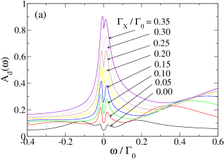
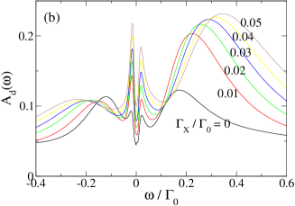
Figure 8: NRG results for the effects of the finite mixing of the orbital quantum number $m$. The parameter values are: $\epsilon_{0}=-0.8D$, $\Gamma_{0}=0.08D$, $U_{mm^{\prime}}=8D$, $\Delta_{\mathrm{orb}}=32T_{K}^{SU(4)}$, and $\Delta_{Z}=2T_{K}^{SU(4)}$.

III.3 Two-Level SU(2) Kondo Effect

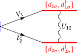
Figure 9: (color online) Schematic of the two-level SU(2)-symmetric Anderson model.

As pointed out in the previous subsection, at the maximum mixing ($V_{0}=V_{X}$) the physics becomes that of the two-level SU(2) Anderson model (see Fig. 9). In this case, the only degree of freedom which is conserved during tunneling is the spin and the total Hamiltonian reads

$$H=\sum_{\alpha=L,R}\sum_{k\sigma}\varepsilon_{\alpha k}a_{\alpha k\sigma}^{\dagger}a_{\alpha k\sigma}\\ \mbox{}+\sum_{\alpha km\sigma}V_{m}\left(a_{\alpha k\sigma}^{\dagger}d_{m\sigma}+d_{m\sigma}^{\dagger}a_{\alpha k\sigma}\right)+H_{D}$$ (35)

or equivalently [see Eq. (4)]

$$H=\sum_{k\sigma}\varepsilon_{k}c_{k\sigma}^{\dagger}c_{k\sigma}\\ \mbox{}+\sum_{km\sigma}V_{m}\left(c_{k\sigma}^{\dagger}d_{m\sigma}+d_{m\sigma}^{\dagger}c_{k\sigma}\right)+H_{D}\,.$$ (36)

As the scaling theory of the Kondo-type Hamiltonian obtained from the two-level Anderson model has been developed in detail in Refs. Kuramoto98a, and Eto04a, , we here focus on the first stage, which highlights the difference between the two-level SU(2)-symmetric Anderson model and the SU(4)-symmetric Anderson model. Finally, the physical arguments based on the perturbative RG theory will be examined quantitatively by means of the NRG method.

As we integrate out the electronic states in the ranges $[-D,-(D-\delta{D})]$ and $[D-\delta{D},D]$ of the conduction band, the dot Hamiltonian (1a) evolves as

$$H_{D}=\sum_{m\sigma}\epsilon_{m\sigma}d_{m\sigma}^{\dagger}d_{m\sigma}-t\sum_{\sigma}\left(d_{1\sigma}^{\dagger}d_{2\sigma}+d_{2\sigma}^{\dagger}d_{1\sigma}\right)\\ \mbox{}+\sum_{(m,\sigma)\neq(m^{\prime},\sigma^{\prime})}U_{mm^{\prime}}n_{m\sigma}n_{m^{\prime}\sigma^{\prime}}$$ (37)

with other terms in the total Hamiltonian (36) kept unchanged. Notice here the appearance of a new term in $t$, i.e., a direct transition between the two orbitals $m=1$ and $2$. Scaling of the parameters $\epsilon_{m\sigma}$ and $t$ are governed by the RG equations

$$\frac{d\epsilon_{m\sigma}}{d\ln D}=-\frac{2}{\pi}\Gamma_{m}\,$$ (38)

and

$$\frac{dt}{d\ln D}=-\frac{2}{\pi}\sqrt{\Gamma_{1}\Gamma_{2}}\,,$$ (39)

respectively.

Figure 10: (color online) Scaling of the single-particle energy level $\epsilon_{d}$, to be compared with $\epsilon_{m\sigma}$ in Eq. (38), of the single-level Anderson model. $\epsilon_{d}^{*}=\epsilon_{d}(D=\Gamma)$ is a scale-invariant quantity.

The RG equation (38) for the single-particle energy levels $\epsilon_{m\sigma}$ is the same as that in the usual single-level Anderson modelHaldane78a ; Haldane78b (the corresponding RG flow diagram is shown in Fig. 10). However, due to the direct transition $t$ emerging from the RG equation (39), $\epsilon_{m\sigma}$ are not relevant to the Kondo effect [they are not the eigenvalues of $H_{D}$ in Eq. (37)]. To find the relevant energy level(s) directly involved in the Kondo effect, one may diagonalize $H_{D}$ in Eq. (37) by means of the canonical transformation

$$\begin{bmatrix}d_{+,\sigma}\\ d_{-,\sigma}\end{bmatrix}=\begin{bmatrix}\phantom{-}\cos(\theta/2)&\sin(\theta/2)\\ -\sin(\theta/2)&\cos(\theta/2)\end{bmatrix}\begin{bmatrix}d_{1\sigma}\\ d_{2\sigma}\end{bmatrix}\,,$$ (40)

where the angle $\phi$ is defined by the relation

$$\tan\theta\equiv\frac{t}{\epsilon_{2}-\epsilon_{1}}\,.$$ (41)

The dot Hamiltonian in Eq. (37) then takes the form

$$H_{D}=\sum_{\mu=\pm}\sum_{\sigma}\epsilon_{\mu}d_{\mu\sigma}^{\dagger}d_{\mu\sigma}+\sum_{(m,\sigma)\neq(m^{\prime},\sigma^{\prime})}U_{mm^{\prime}}n_{m\sigma}n_{m^{\prime}\sigma^{\prime}}\,$$ (42)

with

$$\epsilon_{\mu=\pm}=\frac{1}{2}(\epsilon_{1}+\epsilon_{2})\mp\frac{1}{2}\sqrt{(\epsilon_{1}-\epsilon_{2})^{2}+t^{2}}\,.$$ (43)

At the same time, the canonical transformation in Eq. (40) also changes the coupling term in the total Hamiltonian in Eq. (36) to

$$H_{T}=\sum_{\mu=\pm}\sum_{k\sigma}V_{\mu}\left(c_{k\sigma}^{\dagger}d_{\mu\sigma}+d_{\mu\sigma}^{\dagger}c_{k\sigma}\right)$$ (44)

with $V_{\pm}$ defined by

$$\begin{bmatrix}V_{+}\\ V_{-}\end{bmatrix}=\begin{bmatrix}\phantom{-}\cos(\theta/2)&\sin(\theta/2)\\ -\sin(\theta/2)&\cos(\theta/2)\end{bmatrix}\begin{bmatrix}V_{1}\\ V_{2}\end{bmatrix}\,.$$ (45)

Accordingly, the tunneling rates $\Gamma_{\pm}\equiv\pi\rho_{0}|V_{\pm}|^{2}$ of the effective orbital levels $\epsilon_{\pm,\sigma}$ are given by

$$\Gamma_{\pm}=\frac{1}{2}(\Gamma_{1}+\Gamma_{2})\pm\sqrt{\Gamma_{1}\Gamma_{2}}\sin\theta+\frac{1}{2}(\Gamma_{1}-\Gamma_{2})\cos\theta\,.$$ (46)

Figure 11: (color online) Scaling of the two-level SU(2)-symmetric Anderson model. The arrowed lines indicate RG flows of the effective single-particle energy levels $\epsilon_{\pm}$ [see Eq. (43)] and the widths of the shadowed regions around $\epsilon_{\pm}$ the RG flow of $\Gamma_{\pm}$ [see Eq. (46)]. The mean of $\Gamma_{1}$ and $\Gamma_{2}$ is denoted by $\Gamma_{0}$.

Figure 11 shows the scaling of $\epsilon_{\pm}$ (arrowed lines) and $\Gamma_{\pm}$ (widths of the shadowed regions around $\epsilon_{\pm}$), governed by Eqs. (38), (39), (43), and (46). Note that the effective single-particle energy levels $\epsilon_{\pm}$ always repel each other,Boese02a and the hybridization $\Gamma_{+}$ ($\Gamma_{-}$) of the lower (upper) level $\epsilon_{+}$ ($\epsilon_{-}$) always increases (decreases). Essential in this scaling property of the two-level Anderson model is the direct transition $t$ between the orbitals $m=1$ and $2$, mediated by the conduction band.

The scaling of $\epsilon_{\pm}$ and $\Gamma_{\pm}$ stops when the lower level $\epsilon_{+}$ becomes comparable with $D$ ($\epsilon_{+}\simeq D$); see Fig. 11. Then the charge fluctuations are highly suppressed and the occupation of the lower level becomes close to unity ($\left\langle\textstyle n_{+}\right\rangle\approx 1$). Therefore, only the lower level $\epsilon_{+}$ gets involved in the Kondo physics, and hence the resulting Kondo effect is identical to the usual SU(2) Kondo effect. To be more specific, let us consider the two limiting cases, $|\epsilon_{1}-\epsilon_{2}|\gg\Gamma_{0}$ and $|\epsilon_{1}-\epsilon_{2}|\ll\Gamma_{0}$, assuming

$$|\Gamma_{1}-\Gamma_{2}|\ll\Gamma_{0}\equiv(\Gamma_{1}+\Gamma_{2})/2\,.$$ (47)

Since $t\sim\Gamma_{0}$, one has

$$\theta\approx\begin{cases}\pi/2\,,&|\epsilon_{1}-\epsilon_{2}|\ll\Gamma_{0}\,;\\ 0\,,&|\epsilon_{1}-\epsilon_{2}|\gg\Gamma_{0}\,,\end{cases}$$ (48)

or equivalently,

$$\Gamma_{+}\approx\begin{cases}2\Gamma_{0}\,,&|\epsilon_{1}-\epsilon_{2}|\ll\Gamma_{0}\,;\\ \Gamma_{0}\,,&|\epsilon_{1}-\epsilon_{2}|\gg\Gamma_{0}\,.\end{cases}$$ (49)

This implies that when the two orbital levels are nearly degenerate ($|\epsilon_{1}-\epsilon_{2}|\ll\Gamma_{0}$), the Kondo temperatureHaldane78a ; Haldane78b is enhanced exponentially:

$$T_{K}\simeq\frac{1}{2}\sqrt{2\Gamma_{0}D}\exp\left[+\frac{\pi\epsilon_{0}}{2\Gamma_{0}}\right]\,,$$ (50)

[with $\epsilon_{0}\equiv(\epsilon_{1}+\epsilon_{2})/2$] compared with the single-level case (i.e., $|\epsilon_{1}-\epsilon_{2}|\gg\Gamma_{0}$)

$$T_{K}^{0}\simeq\frac{1}{2}\sqrt{\Gamma_{0}D}\exp\left[+\frac{\pi\epsilon_{0}}{\Gamma_{0}}\right]\,.$$ (51)

In the limit of nearly degenerate levels ($|\epsilon_{1}-\epsilon_{2}|\ll\Gamma_{0}$), the upper level $\epsilon_{-}$ is located at distance smaller than $\Gamma_{+}$ from the lower level $\epsilon_{+}$ [$(\epsilon_{-}-\epsilon_{+})\lesssim\Gamma_{+}$; see the upper panel in Fig. 11] and the transition from $\epsilon_{+}$ to $\epsilon_{-}$ is allowed in general. Indeed, this effect can be taken into account by a proper SW transformation including both levels and scaling of the resulting Kondo-like Hamiltonian,Kuramoto98a ; Eto04a and gives rise to a bump structure at $\omega=\Delta_{\mathrm{eff}}$ above the Fermi energy $E_{F}$ of the leads, with $\Delta_{\mathrm{eff}}$ given by Boese02a (with $\epsilon_{1\sigma}=\epsilon_{2\sigma}$ initially)

$$\Delta_{\mathrm{eff}}\sim\frac{2\Gamma_{0}}{\pi}\ln\frac{D}{\Gamma_{0}}\,$$ (52)

in the single-particle excitation spectrum $A_{d}(\omega)$ in Fig. 12; see below.

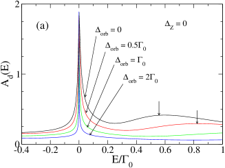
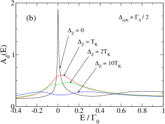
Figure 12: (color online) Total single-particle excitation spectrum $A_{d}(\omega)$ with (a) only the orbital degeneracy lifted ($\Delta_{\mathrm{orb}}\neq 0$, $\Delta_{Z}=0$) and (b) both the orbital and spin degeneracies lifted ($\Delta_{\mathrm{orb}},\Delta_{Z}\neq 0$). The short vertical arrows indicate the transition from $\epsilon_{+}$ to $\epsilon_{-}$, whose excitation energy is given by $\Delta_{\mathrm{eff}}$ [see Eq. (52)]. The parameter values are: $\epsilon_{0}=-0.8D$, $\Gamma_{0}=0.1D$, and $U_{mm^{\prime}}=8D$.

Again, all the interpretations made above on the basis of the perturbative RG are confirmed with the NRG method. Figure 12 shows the total spectral density $A_{d}(E)$. One can see that as $\Delta_{\mathrm{orb}}$ increases with $\Delta_{Z}=0$, the Kondo peak gets sharper, i.e., the enhancement of the Kondo temperature $T_{K}$ in Eq. (50) diminishes for $\Delta_{\mathrm{orb}}\geq\Gamma_{0}$; see Fig. 12(a). Notice that the bump above the Fermi energy originates from the excitation via the transition from the lower level $\epsilon_{+}$ to the higher one $\epsilon_{-}$, and is thus located at $E=\Delta_{\mathrm{eff}}$ [see Eq. (52]. When we allow $\Delta_{Z}$ finite as well, the Kondo peak then splits into two because of the Zeeman splitting.Meir93a ; Wingreen94a

IV Slave-Boson treatment

In order to confirm our previous results and obtain analytical expressions for intermediate mixing, we also use slave boson techniques. In particular, the SBMF approach, which provides a good approximation in the strong coupling limit $T\ll T_{K}$, allows us to obtain analytical expressions for the Kondo temperature and the Kondo peak position for arbitrary mixing. Our SBMFT results are complemented with the NCA, which takes into account both thermal and charge fluctuations in a self-consistent manner.

At equilibrium it is convenient to change into a representation in terms of the symmetric (even) and antisymmetric (odd) combinations of the localized and delocalized orbital channels. izu Thus the even-odd transformation consists of $a_{k,1(2),\sigma}=(c_{k_{e}\sigma}\pm ic_{k_{o}\sigma})\sqrt{2}$ and $d_{1(2)\sigma}=(d_{e\sigma}\pm id_{o\sigma})/\sqrt{2}$. In this basis the Hamiltonian in Eq. (3) reads

$$H=\sum_{\sigma,\nu=e,o}\epsilon_{k_{\nu}}c_{k_{\nu},\sigma}^{\dagger}c_{k_{\nu},\sigma}+\sum_{\sigma,\nu=e,o}\varepsilon_{\nu\sigma}d_{\nu,\sigma}^{\dagger}d_{\nu,\sigma}\\ +\sum_{\nu=e,o}Un_{\nu\downarrow}n_{\nu\uparrow}+Un_{e}n_{o}+V_{e}\sum_{k_{e},\sigma}\left(c_{k_{e},\sigma}^{\dagger}d_{e\sigma}+h.c\right)\\ +V_{o}\sum_{k_{o},\sigma}\left(c_{k_{o},\sigma}^{\dagger}d_{o\sigma}+h.c.\right)\,,$$ (53)

where, again we have taken $V_{0}=V_{1,1}=V_{2,2}$, $V_{X}=V_{1,2}=V_{2,1}$, $U_{m,m^{\prime}}=U$, and $\varepsilon_{\nu,\sigma}=\varepsilon_{0,\sigma}$. The occupation per channel and spin is given by $n_{\nu\sigma}=d_{\nu\sigma}^{\dagger}d_{\nu\sigma}$ and the total occupation per channel is $n_{\nu}=\sum_{\sigma}n_{\nu\sigma}$. The tunneling amplitudes for each channel are given by $V_{e}\equiv V_{0}+V_{X}$ and $V_{o}\equiv V_{0}-V_{X}$. In order to normalize the total tunneling rate, we take, for the diagonal and off-diagonal tunneling amplitudes, $V_{0}=V\cos\phi$ and $V_{X}=V\sin\phi$, namely $V_{e}=V(\cos\phi+\sin\phi)$ and $V_{o}=V(\cos\phi-\sin\phi)$. Notice that one needs $\phi\in[0,\pi/4]$ in order to have always $V_{o}$ positively defined. There exist two very different situations, namely (i) $\phi=0$, where there are only tunneling processes that conserve the orbital index, and (ii) $\phi=\pi/4$, where the mixing and no mixing tunneling amplitudes are the same.

Now we write the physical fermionic operator as a combination of a pseudofermion operator and a boson operator as follows: $d_{\nu\sigma}=b^{\dagger}f_{\nu\sigma}$, where the pseudofermion operator $f_{\nu,\sigma}$ annihilates one “occupied state” in the $\nu$th localized orbital and the boson operator $b^{\dagger}$ creates an “empty state”. Quite generally, the intra-/inter-Coulomb interaction is very large and we can safely take the limit $U\rightarrow\infty$. This fact enforces the constraint $\sum_{\nu\sigma}f_{\nu\sigma}^{{\dagger}}f_{\nu\sigma}+b^{\dagger}b=1$ that prevents the accommodation of two electrons at the same time in either the same orbital or different orbitals. This constraint is treated with a Lagrange multiplier.

$$H_{\mathrm{SB}}=\sum_{\sigma,\nu=e,o}\epsilon_{k_{\nu}}c_{k_{\nu},\sigma}^{\dagger}c_{k_{\nu},\sigma}+\sum_{\sigma,\nu=e,o}\varepsilon_{0,\sigma}f_{\nu,\sigma}^{\dagger}f_{\nu,\sigma}+\frac{\overline{V}_{\nu}}{\sqrt{N}}\sum_{k,\sigma,\nu=e,o}\,\left(c_{k_{\nu},\sigma}^{\dagger}b^{\dagger}f_{\nu,\sigma}+h.c.\right)\\ \mbox{}+\lambda\left(\sum_{\nu,\sigma}f_{\nu,\sigma}^{\dagger}f_{\nu,\sigma}+b^{\dagger}b-1\right)\,.$$ (54)

Notice that we have rescaled the tunneling amplitudes $V_{e(o)}\to\sqrt{N}\overline{V}_{e(o)}$ according to the spirit of a $1/N$-expansion (where $N$ is the total degeneracy of the localized orbital).

Our next task is to solve this Hamiltonian, which is rather complicated due to the presence of the three operators in the tunneling part and the constrain. In order to do this we employ two approaches that describe two different physical regimes. The first one is the SBMFT approach which describes properly the low-temperature strong coupling regime. This SBMFT provides a good approximation in the deep Kondo limit, namely in case that only spin fluctuations are taken into account. The NCA, on the other hand, takes into account both thermal and charge fluctuations in a self-consistent manner. It is well known that the NCA fails in describing the low-energy strong coupling regime. Nevertheless, the NCA has proven to give reliable results at temperatures down to a fraction of $T_{K}$.

IV.1 Slave-boson Mean-Field Theory

We begin with the discussion of the mean-field approximation of Eq. (54). The merit of this approach is its simplicity while capturing the main physics in the pure Kondo regime. It has been successfully applied to investigate the out-of-equilibrium Kondo effect eto01 ; dong02 ; ros03 ; avish03 and double quantum dots, geo99 ; ram00 ; ros02 ; ram03 ; ros05 just to mention a few. This approach corresponds to taking the lowest order $\mathscr{O}(1)$ in the $1/N$ expansion, where the boson operator $b(t)$ is replaced by its classical (nonfluctuating) average, i.e., $b(t)/\sqrt{N}\rightarrow\langle b\rangle/\sqrt{N}\equiv\tilde{b},$ thereby neglecting charge fluctuations. In the limit $N\rightarrow\infty$, this approximation becomes exact. The corresponding mean-field Hamiltonian is given by

$$H_{\mathrm{MF}}=\sum_{\sigma,\nu=e,o}\epsilon_{k_{\nu}}c_{k_{\nu},\sigma}^{\dagger}c_{k_{\nu},\sigma}+\sum_{\nu,\sigma}\tilde{\varepsilon}_{0,\sigma}f_{\nu,\sigma}^{\dagger}f_{\nu,\sigma}\\ \mbox{}+\sum_{\nu,k,\sigma}\left(\tilde{V}_{\nu}\,c_{\nu,k,\sigma}^{\dagger}f_{\nu,\sigma}+h.c.\right)\\ \mbox{}+\lambda\left(\sum_{\nu,\sigma}f_{\nu,\sigma}^{\dagger}f_{\nu,\sigma}+N|\tilde{b}|^{2}-1\right)\,,$$ (55)

where $\tilde{V}_{\nu}=\overline{V}_{\nu}\tilde{b}=V_{\nu}\langle b\rangle$ and $\tilde{\varepsilon}_{0,\sigma}=\varepsilon_{0,\sigma}+\lambda$ are the renormalized tunneling amplitude and the renormalized orbital level, respectively. The two mean-field parameters $\tilde{b}$ and $\lambda$ are to be determined through the mean-field equations, which are the constraint

$$\sum_{\nu,\sigma}\langle f^{\dagger}_{\nu,\sigma}(t)f_{\nu,\sigma}(t)\rangle+N|\tilde{b}|^{2}=1$$ (56)

and the equation of motion for the boson field

$$\sum_{\nu,k,\sigma}\tilde{V}_{\nu}\left\langle c_{k_{\nu},\sigma}^{\dagger}(t)f_{\nu,\sigma}(t)\right\rangle+\lambda N|\tilde{b}|^{2}=0\,.$$ (57)

The Green function for the $\nu\,(=e,o$) localized orbital and the corresponding lesser lead-orbital Green function are given by $G^{<}_{\nu,\sigma}(t-t^{\prime})=-i\langle f^{\dagger}_{\nu,\sigma}(t^{\prime})f_{\nu,\sigma}(t)\rangle$ and $G^{<}_{\nu,\sigma,k_{\nu},\sigma}(t-t^{\prime})=-i\langle c^{\dagger}_{k_{\nu},\sigma}(t^{\prime})f_{\nu,\sigma}(t)\rangle$, respectively. Expressing the mean-field equations in terms of these nonequilibrium Green functions, we obtain Eqs. (56) and (57) in the form

$$\sum_{\sigma}G^{<}_{\nu,\sigma}(t,t)+N|\tilde{b}|^{2}=1\,,$$ (58a)

$$\sum_{\nu,k,\sigma}\tilde{V}_{\nu}G^{<}_{\nu,\sigma;k_{\nu},\sigma}(t,t)+\lambda N|\tilde{b}|^{2}=0\,.$$ (58b)

In order to solve the set of mean-field equations, we proceed as follows: First, we employ analytic continuation rules to the equation of motion for the time-ordered Green functions $G^{t}_{\nu,\sigma}(t-t^{\prime})=-i\langle T_{C}\{f^{\dagger}_{\nu\sigma}(t^{\prime})f_{\nu\sigma}(t)\}\rangle$ and $G^{t}_{\nu,\sigma;k_{\nu},\sigma}(t-t^{\prime})=-i\langle T_{C}\{c^{\dagger}_{k_{\nu},\sigma}(t^{\prime})f_{\nu,\sigma}(t)\}\rangle$, where $T_{C}$ denotes the time-ordering operator along a complex time contour. lan76 Second, we use the equation of motion technique to relate the lead-orbital Green function with the orbital Green function. Finally, we rewrite the mean-field equations in the frequency domain (taking $\varepsilon_{0,\sigma}=\varepsilon_{0}$):

$$|\tilde{b}^{2}|-\frac{1}{N}\sum_{\nu,\sigma}\int\frac{d\epsilon}{2\pi i}\,G_{\nu\sigma}^{<}(\epsilon)=\frac{1}{N}\,,$$ (59a)

$$\lambda|\tilde{b}|^{2}+\frac{1}{N}\sum_{\nu,\sigma}\int\frac{d\epsilon}{2\pi i}\,G_{\nu\sigma}^{<}(\epsilon)(\varepsilon_{0}-\tilde{\varepsilon}_{0})=0\,.$$ (59b)

The integrals in Eq. (59) can be carried out analytically by introducing a Lorentzian cutoff $\rho(\epsilon)=D(\epsilon^{2}+D^{2})^{-1}$ for the DOS in the leads and the lesser orbital Green function $G_{\nu}^{<}(\epsilon)=2i\tilde{\Gamma}_{\nu}f(\epsilon)/[(\epsilon-\tilde{\varepsilon}_{0})^{2}+\tilde{\Gamma}_{\nu}^{2}]$ with $\tilde{\Gamma}_{\nu}=\overline{\Gamma}_{\nu}|\tilde{b}|^{2}$ and the Fermi distribution function $f(\epsilon)$:

$$\frac{2}{\pi N}\mathrm{Im}\left[\ln\left(\frac{\tilde{\varepsilon}_{0}+i\tilde{\Gamma}_{e}}{D}\right)\right]+\frac{2}{\pi N}\mathrm{Im}\left[\ln\left(\frac{\tilde{\varepsilon}_{0}+i\tilde{\Gamma}_{o}}{D}\right)\right]$$

$$=\frac{1}{N}-|\tilde{b}|^{2}\,,$$ (60a)

$$\frac{2\tilde{\Gamma}_{e}}{\pi N}{\rm Re}\left[\ln\left(\frac{\tilde{\varepsilon}_{0}+i\tilde{\Gamma}_{e}}{D}\right)\right]+\frac{2\tilde{\Gamma}_{o}}{\pi N}{\rm Re}\left[\ln\left(\frac{\tilde{\varepsilon}_{0}+i\tilde{\Gamma}_{o}}{D}\right)\right]$$

$$=-\lambda|\tilde{b}|^{2}\,.$$ (60b)

In the deep Kondo limit, where $N^{-1}-|\tilde{b}|^{2}\approx N^{-1}$ and $-\lambda\approx\varepsilon_{0}$, these equations obtain the forms:

$${\rm Im}\left[\ln\left(\frac{\tilde{\varepsilon}_{0}+i\tilde{\Gamma}_{e}}{D}\right)\right]+{\rm Im}\left[\ln\left(\frac{\tilde{\varepsilon}_{0}+i\tilde{\Gamma}_{o}}{D}\right)\right]$$

$$=\frac{\pi}{2}\,,$$ (61a)

$$\Gamma_{e}{\rm Re}\left[\ln\left(\frac{\tilde{\varepsilon}_{0}+i\tilde{\Gamma}_{e}}{D}\right)\right]+\Gamma_{o}{\rm Re}\left[\ln\left(\frac{\tilde{\varepsilon}_{0}+i\tilde{\Gamma}_{o}}{D}\right)\right]$$

$$=\frac{\pi\varepsilon_{0}}{2}\,,$$ (61b)

where $\Gamma_{\nu}=\overline{\Gamma}_{\nu}/N$ is the original rate for the $\nu\,(=e,o)$ channel. Using the parametrization $V_{e}=V(\cos\phi+\sin\phi)$ and $V_{o}=V(\cos\phi-\sin\phi)$, the tunneling rates read $\Gamma_{e}=\pi V^{2}\rho(1+\sin 2\phi)=\Gamma(1+\sin 2\phi)$ and $\Gamma_{o}=\rho=\pi V^{2}\rho(1-\sin 2\phi)=\Gamma(1-\sin 2\phi)$. Taking $\sin 2\phi=\beta$ with $\beta\in[0,1]$ (notice that $0\leq\sin 2\phi\leq 1$ for $\phi\in[0,\pi/4]$), we parametrize the even and odd rates as $\Gamma_{e}=(1+\beta)\Gamma$ and $\Gamma_{o}=(1-\beta)\Gamma$, respectively. Accordingly, the case $\beta\neq 0$ accounts for the process where even and odd channels are not coupled equally to the lead electrons or equivalently, the process where the orbital index is not conserved. In terms of the new notation, the mean-field equations can be written in a compact way:

$${\rm ln}\left[\frac{\tilde{\varepsilon}_{0}+i\tilde{\Gamma}_{e}}{D}\right]+{\rm ln}\left[\frac{\tilde{\varepsilon}_{0}+i\tilde{\Gamma}_{o}}{D}\right]+{\rm ln}\left[\frac{\tilde{\varepsilon}_{0}^{2}+\tilde{\Gamma}_{e}^{2}}{\tilde{\varepsilon}_{0}^{2}+\tilde{\Gamma}_{o}^{2}}\right]^{\beta/2}\\ =i\frac{\pi}{2}+\frac{\pi\varepsilon_{0}}{\Gamma_{e}+\Gamma_{o}}\,,$$ (62)

or equivalently,

$$[\tilde{\varepsilon}_{0}+i\tilde{\Gamma}_{e}][\tilde{\varepsilon}_{0}+i\tilde{\Gamma}_{o}]\left[\frac{\tilde{\varepsilon}_{0}^{2}+\tilde{\Gamma}_{e}^{2}}{\tilde{\varepsilon}_{0}^{2}+\tilde{\Gamma}_{o}^{2}}\right]^{\beta/2}=iD^{2}e^{\pi\varepsilon_{0}(\Gamma_{e}+\Gamma_{o})^{-1}}\,,$$ (63)

the real and imaginary parts of which read

$$[\tilde{\varepsilon}_{0}^{2}-\tilde{\Gamma}_{e}\tilde{\Gamma}_{o}]\left[\frac{\tilde{\varepsilon}_{0}^{2}+\tilde{\Gamma}_{e}^{2}}{\tilde{\varepsilon}_{0}^{2}+\tilde{\Gamma}_{o}^{2}}\right]^{\beta/2}=0\,,$$ (64a)

$$\tilde{\varepsilon}_{0}(\tilde{\Gamma}_{e}+\tilde{\Gamma}_{o})\left[\frac{\tilde{\varepsilon}_{0}^{2}+\tilde{\Gamma}_{e}^{2}}{\tilde{\varepsilon}_{0}^{2}+\tilde{\Gamma}_{o}^{2}}\right]^{\beta/2}=D^{2}e^{\pi\varepsilon_{0}(\Gamma_{e}+\Gamma_{o})^{-1}}\,.$$ (64b)

It is obvious that Eq. (64a) has the solution $\tilde{\varepsilon}_{0}=\pm\sqrt{\tilde{\Gamma}_{e}\tilde{\Gamma}_{o}}$, among which only the positive root satisfies Eq. (64b). Substituting this result in Eq. (64b), we arrive after some algebra at

$$|\tilde{b}|^{2}=\frac{D}{\sqrt{2}}\frac{1}{N\Gamma}\frac{(1-\beta)^{\frac{\beta-1}{4}}}{(1+\beta)^{\frac{\beta+1}{4}}}\,e^{(\pi\varepsilon_{0}/2)(\Gamma_{e}+\Gamma_{o})^{-1}}.$$ (65)

Using the previous result, we may define the Kondo temperature for each channel as: hew93

$$T_{K}^{e} \equiv \sqrt{\tilde{\varepsilon}_{0}^{2}+\tilde{\Gamma}_{e}^{2}}=\frac{(1-\beta)^{\frac{\beta-1}{4}}}{(1+\beta)^{\frac{\beta-1}{4}}}De^{(\pi\varepsilon_{0}/2)(\Gamma_{e}+\Gamma_{o})^{-1}}\,,$$

$$T_{K}^{o} \equiv \sqrt{\tilde{\varepsilon}_{0}^{2}+\tilde{\Gamma}_{o}^{2}}=\frac{(1-\beta)^{\frac{\beta+1}{4}}}{(1+\beta)^{\frac{\beta+1}{4}}}De^{(\pi\varepsilon_{0}/2)(\Gamma_{e}+\Gamma_{o})^{-1}}\,,$$ (66)

and obtain the renormalized level position:

$$\tilde{\varepsilon}_{0}=\frac{D}{\sqrt{2}}e^{(\pi\varepsilon_{0}/2)(\Gamma_{e}+\Gamma_{o})^{-1}}\frac{(1-\beta)^{\frac{\beta+1}{4}}}{(1+\beta)^{\frac{\beta-1}{4}}}\,.$$ (67)

Equations (IV.1) and (67), which are the main results of this section, give the Kondo temperatures and level position for arbitrary mixing $\beta$. Note that $\Gamma_{e}+\Gamma_{o}=2\Gamma$ does not depend on $\beta$ and therefore the Kondo temperature depends on the orbital mixing only through the prefactor. While $T_{K}^{e}$ changes very little with $\beta$, $T_{K}^{o}$ reduces down to zero as $\beta\rightarrow 1$ (maximum mixing). Similarly, $\tilde{\varepsilon}_{0}$ goes from $T_{K}\equiv N\Gamma|\tilde{b}|^{2}(\beta=0)=(D/\sqrt{2})\exp(\pi\varepsilon_{0}/4\Gamma)$ to zero, in agreement with the Friedel sum rule. From the above results, we conclude that the odd orbital becomes decoupled at maximum mixing, where we are left with SU(2) Kondo physics arising from spin fluctuations in the even orbital channel. This SU(4)-to-SU(2) transition as mixing increases is illustrated in Fig. 2, where the SBMFT parameters are plotted versus $\beta$.

Now we are in position to calculate transport properties. For this purpose, it is more convenient to write SBMFT equations in the matrix form:

$$|\tilde{b}^{2}|-\frac{1}{N}\int\frac{d\epsilon}{2\pi i}\,{\rm Tr}\hat{G}^{<}(\epsilon)=\frac{1}{N}\,,$$ (68a)

$$\lambda|\tilde{b}|^{2}+\frac{1}{N}\int\frac{d\epsilon}{2\pi i}\,{\rm Tr}\{\hat{\Sigma}^{r}\hat{G}^{<}(\epsilon)+\hat{\Sigma}^{<}\hat{G}^{a}(\epsilon)\}=0\,,$$ (68b)

where we are back to the original basis and the trace includes also the sum over spin indices. Here, $\hat{G}^{<}$ is the lesser matrix orbital Green function, which is related to the advanced $\hat{G}^{a}$ and retarded $\hat{G}^{r}$ matrix Green functions through the expression

$$\hat{G}^{<}=\hat{G}^{a}\hat{\Sigma}^{<}\hat{G}^{r}$$ (69)

with $\hat{\Sigma}^{<}$ being the lesser matrix self-energy. The explicit expressions for these matrices are

$$\hat{G}^{a}(\epsilon) = \frac{1}{(\epsilon-\tilde{\varepsilon}_{0}-iT_{K})^{2}+\beta^{2}T_{K}^{2}}$$ (70)

$$\times \left(\begin{array}[]{cc}\epsilon-\tilde{\varepsilon}_{0}-iT_{K}&i\beta T_{K}\\ i\beta T_{K}&\epsilon-\tilde{\varepsilon}_{0}-iT_{K}\end{array}\right)\,$$ (73)

and $\hat{G}^{r}$ given by direct complex conjugation of $\hat{G}^{a}$). The lesser matrix self-energy reads

$$\hat{\Sigma}^{<}=-2i\left[f_{L}(\epsilon)+f_{R}(\epsilon)\right]\times\left(\begin{array}[]{cc}T_{K}&\beta T_{K}\\ \beta T_{K}&T_{K}\end{array}\right)$$ (76)

whereas in the same way the retarded matrix self-energy is

$$\hat{\Sigma}^{r}=-i\hat{\Gamma}=-i\left(\begin{array}[]{cc}T_{K}&\beta T_{K}\\ \beta T_{K}&T_{K}\end{array}\right)\,.$$ (79)

Inserting Eqs. (70) and (76) in Eq. (69), we obtain the lesser orbital Green function:

$$\hat{G}^{<}=\frac{-iT_{K}}{(\epsilon-\tilde{\varepsilon}_{0})^{4}+2(1+\beta^{2})T_{K}^{2}(\epsilon-\tilde{\varepsilon}_{0})^{2}+(\beta^{2}-1)^{2}T_{K}^{4}}\left(\begin{array}[]{cc}(\epsilon-\tilde{\varepsilon}_{0})^{2}+T_{K}(1-\beta^{2})&\beta\left[(\epsilon-\tilde{\varepsilon}_{0})^{2}-T_{K}(1-\beta^{2})\right]\\ \beta\left[(\epsilon-\tilde{\varepsilon}_{0})^{2}-T_{K}(1-\beta^{2})\right]&(\epsilon-\tilde{\varepsilon}_{0})^{2}+T_{K}(1-\beta^{2})\end{array}\right).$$ (82)

Using the explicit expressions of the self-energies and the nonequilibrium Green functions, we write Eq. (68b) in the simple form:

$$\lambda|\tilde{b}|^{2}+\frac{1}{N}\int\frac{d\epsilon}{2\pi i}\,{\rm Tr}\,\hat{G}^{<}(\epsilon)\,(\epsilon-\tilde{\varepsilon}_{0})=0\,.$$ (83)

Solving in a self-consistently way Eqs. (68a) and (83) for each dc bias $V_{\rm dc}$, one gets the behavior of the two renormalized parameters in nonequilibrium conditions.ram00

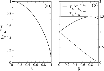
Figure 13: (Color online) Transition from SU(4) to SU(2) Kondo physics as obtained from SBMFT: As the orbital mixing is increased, the SU(4) Kondo effect reduces to the SU(2) spin Kondo effect. This is reflected by (a) the position of the Kondo resonance as well as by (b) the reduction of the odd Kondo temperature down to zero. See the main text.

The electrical current has in appearance the same form as the conventional Landauer-Büttiker current expression for noninteracting electrons:

$$I=\frac{2e}{\hbar}\int\frac{d\epsilon}{2\pi}\mathcal{T}(\epsilon,V_{\rm dc})\left[f_{L}(\epsilon)-f_{R}(\epsilon)\right]\,.$$ (84)

Here caution is needed for a correct interpretation of Eq. (84), since it contains “many-body” effects via the renormalized parameters that have to be determined for each $V_{\rm dc}$ in a self-consistent way. As a result, the transmission $\mathcal{T}(\epsilon,V_{\rm dc})$ possesses, in contrast with the noninteracting case, nontrivial behavior with voltage. The nonlinear conductance is calculated by direct differentiation of Eq. (84) with respect to the bias voltage: $\mathcal{G}\equiv dI/dV_{\rm dc}$. In the limit $V_{\rm dc}\rightarrow 0$ (at equilibrium), the linear conductance $\mathcal{G}_{0}$ is given by the well-known expression:

$$\mathcal{G}_{0}=\frac{2e^{2}}{h}\mathcal{T}(0)\,,$$ (85)

where the transmission is

$$\mathcal{T}(\epsilon)={\rm Tr}\{\hat{G}^{a}\hat{\Gamma}\hat{G}^{r}\hat{\Gamma}\}\,.$$ (86)

Finally, inserting Eqs. (70) and (79) in Eq. (86), one arrives at the explicit formula for the transmission

$$\mathcal{T}(\epsilon)=\frac{2T_{K}^{2}\left[(1+\beta^{2})(\epsilon-\tilde{\varepsilon}_{0})^{2}+T_{K}^{2}(\beta^{2}-1)^{2}\right]}{(\epsilon-\tilde{\varepsilon}_{0})^{4}+2(1+\beta^{2})T_{K}^{2}(\epsilon-\tilde{\varepsilon}_{0})^{2}+(\beta^{2}-1)^{2}T_{K}^{4}}\,,$$ (87)

which is the main result of this part. It is remarkable that the linear conductance $\mathcal{G}_{0}$ does not depend on $\beta$. In particular, for the SU(4) Kondo model ($\beta=0$), the transmission takes the simple form:

$$\mathcal{T}(\epsilon)=\frac{2T_{K}^{2}}{(\epsilon-\tilde{\varepsilon}_{0})^{2}+T_{K}^{2}}\,.$$ (88)

In this case the resonance is pinned at $\epsilon=\tilde{\varepsilon}_{0}=T_{K}$ with the width given by $T_{K}$; this leads to $\mathcal{T}(0)=1$ and in consequence $\mathcal{G}_{0}=2e^{2}/h$. For $\beta=1$ corresponding to the two-level SU(2) Kondo model, Eq. (87) reduces to

$$\mathcal{T}(\epsilon)=\frac{4T_{K}^{2}}{(\epsilon-\tilde{\varepsilon}_{0})^{2}+4T_{K}^{2}}\,,$$ (89)

which leads to the resonance at $\epsilon=\tilde{\varepsilon}_{0}=0$ and again $\mathcal{G}_{0}=2e^{2}/h$ from $\mathcal{T}(0)=1$. As pointed out, this fact makes both Kondo effects indistinguishable through the linear conductance measurement.

All these features are clearly observed in Fig. 14, where the transmission for different amounts of mixing, i.e., different values of $\beta$ is plotted. For $\beta=0$ the transmission peak is located at $T_{K}$ as expected, whereas for $\beta=1$ this moves towards $\epsilon=0$. During the transition from the SU(4) to the two-level SU(2) Kondo model, the transmission gets narrower and develops a “cusp”, signaling competition between even and odd channels. This is manifested by the following from of the transmission:

$$\mathcal{T}(\epsilon)=\frac{(1+\beta)^{2}T_{K}^{2}}{(\epsilon-\tilde{\varepsilon}_{0})^{2}+T_{K}^{2}(1+\beta)^{2}}+\frac{(1-\beta)^{2}T_{K}^{2}}{(\epsilon-\tilde{\varepsilon}_{0})^{2}+T_{K}^{2}(1-\beta)^{2}}\,.$$ (90)

Note that both channels are resonant at the same energy $\tilde{\varepsilon}_{0}$ but have different widths ($\tilde{\Gamma}_{e}$ and $\tilde{\Gamma}_{o}$), which explains the “cusp” behavior. Here we speculate that finite splitting $\delta\varepsilon$ originating from charge fluctuations Manhn-SooPRL04 (not included at the SBMFT level) would give rise to two split resonances for $\beta\neq 0$, namely, $\tilde{\varepsilon}_{0}\rightarrow\tilde{\varepsilon}_{0}^{\pm}=\delta\varepsilon\pm\sqrt{\tilde{\Gamma}_{e}\tilde{\Gamma}_{o}}$. This is confirmed in the next section, where we present results obtained from full NCA calculations including fluctuations. Eventually, for $\beta=1$ the competition does not exist and the transmission does not display the cusp.

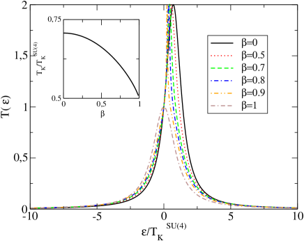
Figure 14: (Color online) Equilibrium SBMFT result: Transmission $\mathcal{T}(\epsilon)$ as a function of the frequency for several values of $\beta$. The left inset displays the Kondo temperature versus $\beta$.

IV.2 Non-crossing approximation Method

The SBMFT suffers from two drawbacks: 1) It leads always to local Fermi liquid behavior and 2) there arises a phase transition (originating from breakdown of the local gauge symmetry of the problem) that separates the low-temperature state from the high-temperature local moment regime. The latter problem may be corrected by including 1/N corrections around the mean-field solution. The non-crossing approximation (NCA) NCAneq1 ; NCAneq2 ; NCAneq3 is the lowest-order self-consistent, fully conserving, and $\Phi$ derivable theory in the Baym sense Baym which includes such corrections. Without entering into details of the theory, we just mention that the boson fields in Eq. (54), treated as averages in the previous subsection ($b(t)/\sqrt{N}\rightarrow\langle b\rangle/\sqrt{N}\equiv\tilde{b}$), are now treated as fluctuating quantum objects. In particular, one has to derive self-consistent equations of motion for the time-ordered double-time Green function (with subindexes omitted):

$$iG(t,t^{\prime}) \equiv \langle T_{c}f(t)f^{\dagger}(t^{\prime})\rangle\,,$$

$$iB(t,t^{\prime}) \equiv \langle T_{c}b(t)b^{\dagger}(t^{\prime})\rangle,$$ (91)

or in terms of their analytic pieces,

$$iG(t,t^{\prime}) = G^{>}(t,t^{\prime})\theta(t-t^{\prime})-G^{<}(t,t^{\prime})\theta(t^{\prime}-t)\,,$$

$$iB(t,t^{\prime}) = B^{>}(t,t^{\prime})\theta(t-t^{\prime})+B^{<}(t,t^{\prime})\theta(t^{\prime}-t).$$ (92)

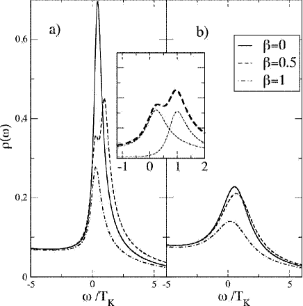
Figure 15: (Color online) NCA results: Density of states around $\varepsilon=0$ at $T=0.25T_{K}$ (left) and $T=T_{K}$ (right) for several values of $\beta$. The inset shows a close-up of the $\beta=0.5$ curve (thick dashed), together with the individual even and odd channel contributions (thin dashed).

A rigorous and well-established way to derive these equations of motion was introduced,Kadan and related to other non-equilibrium methods such as the Keldysh method.lan76 Here, we just present numerical results of the NCA equations for our problem and refer interested readers to Refs. ram03, ; NCAneq1, ; NCAneq2, ; NCAneq3, for details.

In particular, the DOS is given by

$$\rho(\varepsilon)=-\frac{1}{\pi}\sum_{\nu=e,o,\sigma}\mathrm{Im}[A^{r}_{\nu\sigma}(\varepsilon)],$$ (93)

where $A^{r}_{\nu\sigma}(\varepsilon)$ is the Fourier transform of the retarded Greens function:

$$A^{r}_{\nu\sigma}(t)=G_{\nu,\sigma}^{r}(t)B^{<}(-t)-G^{<}_{\nu\sigma}(t)B^{a}(-t).$$ (94)

The DOS for several values of $\beta$ at two different temperatures is plotted in Fig. 15. Interestingly, the cusp behavior of Fig. 14 in the previous subsection becomes split for the even and odd channels. This is illustrated in the inset, where the curve corresponding to $\beta=0.5$ is plotted together with the individual even and odd channel contributions. As we anticipate, the presence of charge fluctuations induces splitting of $\varepsilon_{0}$ due to the different renormalization arising from different couplings for the even and odd channels $\Gamma_{e/o}$ [see Eqs. (38) and (39)].

V Conclusion

We have considered the single-electron transistor (SET) device with the CNT QD or VQD as the central island in the Kondo regime. In particular we have examined the case where the CNT QD or VQD has a high symmetry so that the orbital quantum numbers are conserved through the system. Emphasis has been paid on how different Kondo physics, the SU(4) Kondo effect or the two-level SU(2) Kondo effect, emerges depending on the extent to which the symmetry is broken in realistic situations. Employed are four different theoretical approaches: the scaling theory, the NRG method, the SBMFT, and the NCA method to address both the linear and non-linear conductance for given external magnetic fields. Our results show that there is no way to distinguish experimentally the SU(4) Kondo effect and the two-level SU(2) effect by means of the linear conductance (which is a low-energy property) alone. The SU(4) Kondo physics, which arises with higher symmetry, can be observed exclusively only by the non-linear conductance (a higher-energy property) in the presence of finite magnetic fields, as in the recent experiment.Jarillo-Herrero05a ; Jarillo-Herrero05b The symmetry breaking (either the orbital anisotropy $1-\Gamma_{2}/\Gamma_{1}$ or the orbital mixing $\Gamma_{X}$) drives the system from the SU(4) Kondo fixed point to the SU(2) Kondo fixed point. At finite yet sufficiently small symmetry breaking, the SU(4) Kondo physics governs the transport in the system at relatively high energies (of the order of the Kondo temperature) while the two-level SU(2) Kondo effect takes it over at extremely low energies. This gives another reason why the indication of the SU(4) Kondo physics should be investigated by means of the non-linear conductance in the presence of external magnetic fields.

Appendix A Numerical Renormalization Group

The Hamiltonian (3) allows both charge fluctuations and spin fluctuations. Charge fluctuations (accompanied by the particle-hole excitations) occurs at high energies while spin fluctuations prevail at low energies. Therefore in order to understand the low-energy properties of the system, it is useful to take the RG approach and to obtain an effective Hamiltonian allowing only the spin fluctuations. One may follow the three-state perturbative RG procedure (scaling theory): One first renormalizes the Anderson-type Hamiltonian (3) until the charge fluctuations are completely suppressedHaldane78a ; Haldane78b (see also Ref. Boese02a, ), performs the SW transformationSchrieffer66a to obtain a Kondo-type Hamiltonian where spin fluctuations are described by the spin operators, and renormalizes further the resulting Kondo-type Hamiltonian.Anderson70a The RG equations for the coupling constants in the Hamiltonian allow one to identify physically interesting fixed points and associated scaling properties.

We follow the standard procedure to implement the NRG calculations, Wilson75a ; Krishna-murthy80a ; Costi94a and evaluate various physical quantities from the recursion relation ($N\geq 0$)

$$\widetilde{H}_{N+1}=\sqrt{\Lambda}\,\widetilde{H}_{N}\\ \mbox{}+\xi_{N+1}\sum_{\mu\sigma}\left(f_{\mu,N,\sigma}^{\dagger}f_{\mu,N+1,\sigma}+h.c.\right)$$ (95)

with the initial Hamiltonian

$$\widetilde{H}_{0}=\frac{1}{\sqrt{\Lambda}}\Biggl{[}\widetilde{H}_{D}+\sum_{\mu m}\sum_{\sigma}\widetilde{V}_{\mu,m}\left(f_{\mu,0,\sigma}^{\dagger}d_{m\sigma}+h.c.\right)\Biggr{]}\,,$$ (96)

where the fermion operators $f_{\mu,N,\sigma}$ have been introduced as a result of the logarithmic discretization and the accompanying canonical transformation, $\Lambda$ is the logarithmic discretization parameter (taken to be $\Lambda=2$),

$$\xi_{N}\equiv\frac{1-\Lambda^{-N}}{\sqrt{[1-\Lambda^{-(2N-1)}][1-\Lambda^{-(2N+1)}]}}\,,$$ (97)

and

$$\widetilde{H}_{D}\equiv\zeta\frac{H_{D}}{D}$$ (98)

with $\zeta=2(1+1/\Lambda)^{-1}$. The coupling constants $\widetilde{V}_{\mu,m}$ have been defined to be

$$\widetilde{V}_{\mu,m}\equiv\sqrt{\frac{2\rho_{0}|V_{\mu,m}|^{2}}{\pi D}}\,,$$ (99)

where $\rho_{0}$ is the density of states of the leads at the Fermi energy. The Hamiltonian $\widetilde{H}_{N}$ in Eq. (95) has been rescaled for numerical accuracy, and the original Hamiltonian is recovered by

$$\frac{H}{D}=\lim_{N\to\infty}\frac{\widetilde{H}_{N}}{\mathscr{S}_{N}}$$ (100)

with $\mathscr{S}_{N}\equiv\zeta\Lambda^{(N-1)/2}.$ At each iteration of the NRG procedure, we calculate the local spectral density,Bulla01a which determines the transport properties through the dot:

$$A_{mm^{\prime}}(\omega)=A_{mm^{\prime}}^{>}(\omega)-A_{mm^{\prime}}^{<}(\omega)$$ (101)

with

$$A_{mm^{\prime};\sigma}^{>}(E) =+\sum_{\alpha}\left\langle\textstyle 0\right|d_{m\sigma}\left|\textstyle\alpha\right\rangle\left\langle\textstyle\alpha\right|d_{m^{\prime}\sigma}^{\dagger}\left|\textstyle 0\right\rangle\delta(E-E_{\alpha}+E_{0})\,,$$ (102a)

$$A_{mm^{\prime};\sigma}^{<}(E) =-\sum_{\alpha}\left\langle\textstyle 0\right|d_{m^{\prime}\sigma}^{\dagger}\left|\textstyle\alpha\right\rangle\left\langle\textstyle\alpha\right|d_{m\sigma}\left|\textstyle 0\right\rangle\delta(E+E_{\alpha}-E_{0})\,,$$ (102b)

where $\left|\textstyle\alpha\right\rangle$ represents the many-body state of the system with energy $E_{\alpha}$ (with $\alpha=0$ corresponding to the ground state).

References

- (1) D. Goldhaber-Gordon, H. Shtrikman, D. Mahalu, D. Abusch-Magder, U. Meirav, and M. A. Kastner, Nature (London) 391, 156 (1998); D. Goldhaber-Gordon, J. Göres, M. A. Kastner, Hadas Shtrikman, D. Mahalu, and U. Meirav, Phys. Rev. Lett. 81, 5225 (1998).
- (2) S. M. Cronenwett, T. H. Oosterkamp, and L. P. Kouwenhoven, Science 281, 540 (1998).
- (3) J. Schmid, J. Weis, K. Eberl, and K. von Klitzing, Physica B 256-258, 182 (1998).
- (4) W. G. van der Wiel, S. De Franceschi, T. Fujisawa, J. M. Elzerman, S. Tarucha, and L. P. Kouwenhoven, Science 289, 2105 (2000).
- (5) S. Sasaki, S. De Franceschi, J. M. Elzerman, W. G. van der Wiel, M. Eto, S. Tarucha, and L. P. Kouwenhoven, Nature (London) 405, 764 (2002).
- (6) J. Park, A. N. Pasupathy, J. I. Goldsmith, C. Chang, Y. Yaish, J. R. Petta, M. Rinkoski, J. P. Sethna, H. D. Abrua, P. L. McEuen, and D. C. Ralph, Nature (London) 417, 722 (2002); W. Liang, M. P. Shores, M. Bockrath, J. R. Long, and H. Park, Nature (London) 417, 725 (2002).
- (7) A. Pasupathy, R. Bialczak, J. Martinek, J. Grose, L. Doney, P. McEuen, and D. Ralph, Science 306, 86 (2004).
- (8) M. R. Buitelaar, T. Nussbaumer, and C. Schönenberger, Phys. Rev. Lett. 89, 256801 (2002).
- (9) P. Jarillo-Herrero, J. Kong, H. S. J. van der Zant, C. Dekker, L. P. Kouwenhoven, and S. De Franceschi, Nature (London) 434, 484 (2005).
- (10) M.-S. Choi, R. López, and R. Aguado, Phys. Rev. Lett. 95, 067204 (2005).
- (11) R. Sakano and N. Kawakami, Phys. Rev. B 73, 155332 (2006).
- (12) E. D. Minot, Y. Yaish, V. Sazonova, and P. L. McEuen, Nature (London) 428, 536 (2004).
- (13) J. Cao, Q. Wang, M. Rolandi, and H. Dai, Phys. Rev. Lett. 93, 216803 (2004).
- (14) S. Sasaki, S. Amaha, N. Asakawa, M. Eto, and S. Tarucha, Phys. Rev. Lett. 93, 017205 (2004).
- (15) Here we focus on quarter filling. For half filling, an interesting quantum phase transition involving SU(4) symmetry has been discussed in M. Galpin, D. Logan and H. R. Krishnamurthy, Phys. Rev. Lett. 94, 186406 (2005).
- (16) P. W. Anderson, J. Phys. C 3, 2436 (1970).
- (17) F. D. M. Haldane, Phys. Rev. Lett. 40, 416 (1978). See also Haldane78b .
- (18) F. D. M. Haldane, Phys. Rev. Lett. 40, 911 (1978).
- (19) K. G. Wilson, Rev. Mod. Phys. 47, 773 (1975).
- (20) H. R. Krishna-murthy, J. W. Wilkins, and K. G. Wilson, Phys. Rev. B 21, 1003 (1980).
- (21) T. A. Costi, A. C. Hewson, and V. Zlatic, J. Phys.: Condens. Matter 6, 2519 (1994).
- (22) W. Hofstetter, Phys. Rev. Lett. 85, 1508 (2000).
- (23) Y. Meir and N. S. Wingreen, Phys. Rev. Lett. 68, 2512 (1992).
- (24) D. C. Langreth, Phys. Rev. 150, 516 (1966).
- (25) Y. Kuramoto, Eur. Phys. J. B 5, 457 (1998).
- (26) M. Eto, J. Phys. Soc. Jpn. 74, 95 (2004) (special issue on “Kondo Effect – 40 Years after the Discovery”).
- (27) D. Boese, W. Hofstetter, and H. Schoeller, Phys. Rev. B 66, 125315 (2002).
- (28) Y. Meir and N. S. Wingreen, Phys. Rev. Lett. 70, 2601 (1993).
- (29) N. S. Wingreen and Y. Meir, Phys. Rev. B 49, 11040 (1994).
- (30) W. Izumida, O. Sasakai, and Y. Shimizu, J. Phys. Soc. Jpn. 66, 717 (1997).
- (31) T. Aono and M. Eto, Phys. Rev. B 63, 125327 (2001).
- (32) B. Dong and X.L. Lei, J. Phys. Condens. Matter 14, 4963 (2002).
- (33) R. López and D. Sánchez, Phys. Rev. Lett. 90, 116602 (2003).
- (34) Y. Avishai, A. Golub, and A. D. Zaikin, Phys. Rev. B 67, 041301 (2003).
- (35) A. Georges and Y. Meir, Phys. Rev. Lett. 82, 3508 (1999).
- (36) R. Aguado and D. C. Langreth, Phys. Rev. Lett. 85, 1946 (2000).
- (37) R. Lopez, R. Aguado, and G. Platero, Phys. Rev. Lett. 89, 136802 (2002); Phys. Rev. B 65, 235305 (2004).
- (38) R. Aguado and D. C. Langreth, Phys. Rev. B 67, 245307 (2003).
- (39) R. Lopez, P. Simon, and Y. Oreg Phys. Rev. Lett. 94, 086602 (2005).
- (40) D. C. Langreth, in Linear and Nonlinear Electron Transport in Solids, Nato ASI, Series B vol. 17, edited by J. T. Devreese and V. E. Van Doren (Plenum, New York, 1976).
- (41) A. C. Hewson, The Kondo Problem to Heavy Fermions (Cambridge University Press, Cambridge, UK, 1993).
- (42) M.-S. Choi, R. López and D. Sánchez, Phys. Rev. Lett. 92, 0506601 (2004).
- (43) D. C. Langreth and P. Nordlander, Phys. Rev. B 43, 2541 (1991).
- (44) N. S. Wingreen and Y. Meir, Phys. Rev. B 49, 11040 (1994)
- (45) M. H. Hettler, J. Kroha, and S. Hershfield, Phys. Rev. Lett. 73, 1967 (1994); Phys. Rev. B 58, 5649 (1998).
- (46) G. Baym and L. P. Kadanoff, Phys. Rev. 124, 287 (1961); G. Baym, Phys. Rev. 127, 1391 (1962).
- (47) L. P. Kadanoff and G. Baym, Quantum Statistical Mechanics (Benjamin, New York, 1962).
- (48) P. Jarillo-Herrero, J. Kong, H. S. J. van der Zant, C. Dekker, L. Kouwenhoven, and S. De Franceschi, Phys. Rev. Lett. 94, 156802 (2005).
- (49) J. R. Schrieffer and P. A. Wolff, Phys. Rev. 149, 491 (1966).
- (50) R. Bulla, T. A. Costi, and D. Vollhardt, Phys. Rev. B 64, 45103 (2001).