Scanning the critical fluctuations
– application to the phenomenology of the two-dimensional XY-model –
Abstract
We show how applying field conjugated to the order parameter, may act as a very precise probe to explore the probability distribution function of the order parameter. Using this ‘magnetic-field scanning’ on large-scale numerical simulations of the critical 2D XY-model, we are able to discard the conjectured double-exponential form of the large-magnetization asymptote.
pacs:
05.50.+q, 64.60.Fr, 75.10.HkIntroduction. –
Derivation of the complete equation of state of a many-body system is generally a formidable task. When the system may appear under various phases at the thermodynamic equilibrium, this problem requires knowledge of the exact probability distribution function (PDF) of its order parameter. Despite a number of attempts, just a few instances are available Kolmogorov . Even the exact PDF for the 2D Ising model is still unknown.
Within this context, the critical point is very particular, since the universality concept tells us that only a limited information is needed to obtain the complete leading critical behavior. For instance, general arguments give precisely the tail of the critical PDF, , for the large values of the order parameter, , namely Bouchaud :
| (1) |
with a positive constant and the magnetic field critical exponent, or the distribution of the zeros of the Ising partition function in the complex magnetic field Yang-Lee (such a partition function is Fourier transform of the PDF).
In the present work, we explain how the real magnetic field can be generally used as a very accurate probe to scan quantitatively the zero-field PDF tail, exemplifying the method with the critical 2D XY-model. By the way, we will see that the popular double-exponential approximation of the PDF for this system cannot be correct, and we provide alternative approximation which is consistent with the critical behavior. Consequently, our results discard possible fundamental connexion between this magnetic model and the field of extremal-values statistics.
Former approximation of the magnetization PDF for the critical 2D XY-model. –
In a series of recent papers Bram1 ; Bram2 ; Bram3 ; holds , it was argued that the PDF of the magnetization of the 2D XY-model at the Berezinskii-Kosterlitz-Thouless (BKT) critical temperature, could be approximated by the generalized Gumbel form:
| (2) |
where the reduced magnetization: is used. From low-temperature spin-wave theory and direct numerical simulations, one obtains Bram2 :
| (3) |
It was regularly noticed Bram2 that the form (2) cannot be the exact solution of the corresponding statistical problem, even if a number of analytical arguments as well as numerical simulations show convincingly that this trial function is indeed close to the exact solution. Moreover, Eq.(2) is appealing, as it suggests connexion between the critical 2D XY-model and the statistics of extreme variables extremes . Therefore, the question of a possible bridge between these two active fields of statistical physics should be examined precisely. On the other hand, Eq.(2) is inconsistent with the general behavior (1), since for the 2D XY-model. The question to know whether relation (1) is true or wrong for this system, is then fundamentally important. We will examine hereafter these two questions.
Two alternative hypothesis. –
We consider the 2D XY-model Bere on a square lattice of size with periodic boundary conditions. The classical spins are confined in the - lattice plane, and they interact according to the Hamiltionian: , where is the ferromagnetic coupling constant and the sum runs over all nearest-neighbor pairs of spins. Eventual critical features are characterized by the singular behavior of the scalar magnetization per site: , which is a non-negative real number. We define also the instantaneous magnetization direction as the angle such that: and .

There is a continuous line of critical points for any temperature below the critical BKT temperature KT . In this region, , the system is critical, and asymptotic (i.e. ) self-similarity results in the so-called first-scaling law nous :
| (4) |
and is a scaling function which depends only on the actual temperature .
Under this form,
the hyperscaling relation, , is automatically realized.
Eq.(4) is a sequel of the standard finite-size scaling theory FFS ,
but it is highly advantageous
that (4) does not require knowledge of any critical exponent.
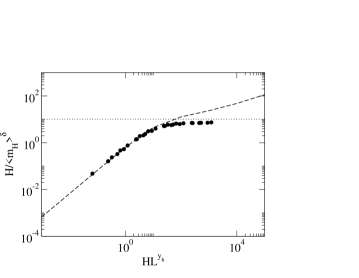
FIG.(1) gives numerical exemplification of the first-scaling law at ,
and illustrates the overall shape of the distribution
(hereafter, the index ‘’ refers to the BKT critical point, ).
We separate the free energy of the 2D XY-system at equilibrium (temperature ) into the sum of a regular part describing the small values of the magnetization, a singular part Widom vanishing as the essential singularity Amit ; Gulacsi when , and a regular part for the large values of the magnetization, namely:
| (5) |
Clearly, discussion on the system behavior can be carried out either through the free energy (5) or the first-scaling law (4), since: constant term.
The regular small- tail. –
As the singular behavior should vanish at the BKT transition, we study first the regular small- behavior of at . Numerical results for are shown on FIG.2 in the form (4). They suggest the leading form:
| (6) |

The singular small- tail. –
We consider now the singular part of the free energy through the combination:
| (7) |
vs the reduced magnetization . The data plotted in FIG.3, suggest a cubic -behavior:
| (8) |
for every , and for the values of smaller than the mean. Moreover, .

The large- tail at the BKT point. –
Instead of using multicanonical Monte-Carlo simulations Berg which need too large system sizes to conclude Hilfer , we consider static in-plane magnetic field, , as a probe to study the features of the PDF for the large values of the magnetization. Indeed, as the intensity of increases, the most probable magnetization, , as well as its mean value, , explores larger values of the PDF tail. We consider two alternative forms for the critical tail, namely:
the ‘Gumbel-like’ shape (2) – noted below: ‘ hypothesis ’ –, which writes in the first-scaling form:
with ( from (3) and Table 1), and . It is the form suggested in Bram1 ; Bram2 ; Bram3 ;
the ‘Weibull-like’ critical shape – noted below: ‘ hypothesis ’ –, which is book :
with a positive parameter, and KosterlitzH .
Let be the direction of with respect to the -axis (i.e. ). According to general thermodynamics, the magnetization PDF is given by: , with the field-less free energy . Therefore, the most probable magnetization, , is the solution of the equation for a given value of . As the instantaneous magnetization direction should coincide with the magnetic field direction for the large systems, we use . Rewritten in terms of the auxiliary variables and , Eqs.(5),(6), with hypothesis or , result respectively in:
| or | |||||
| (10) |
which are implicit equations for the most probable magnetization, , (written in the combination ) vs the magnetic field and the system size (written in the combination ). The constant is such that: .
For the large magnetic field, is expected to be much larger than , that is: . Consequently, the solution of Eq.(The large- tail at the BKT point. –) is:
| (11) |
where is a positive constant.
Within the hypothesis , one has: , such that (10) shows that is asymptotically a constant:
| (12) |
So, increase of with the intense magnetic field should be interpretated as failure of .
Inference from the numerical simulations. –
Both solutions, (11) and (12), are drawn on FIG.4 in comparison with the results of large-scale numerical simulations of the 2D XY-model with the in-plane magnetic field at the BKT temperature. It is clear that the numerical simulations are consistent with the hypothesis , while the double-exponential tail should be discarded. This suggests the following form of the critical PDF for the 2D XY-model:
| (13) |
Below the BKT critical temperature, additional term should appear in the exponential.
In order to understand the origin of the approximation (2), let us change the reduced magnetization according to: . At , and for the small values of (recall that , and that is a rather large number), we obtain:
Writing then , yields Eq.(2), provided the following relations are verified:
| (14) |
So, Eq.(2) appears to be a good approximation around the most probable magnetization, but is inconsistent with the general critical relation , unlike Eq.(13). By the way, the conjectured relation Bram2 writes simply: , that we accept here as a new conjecture (numerically: , see FIG.2).
0.3 16 0.923218 66.958 0.6 16 0.836307 29.249 0.8 16 0.764091 18.260 0.885 16 0.723259 13.907 0.893 16 0.718814 13.467 0.893 32 0.662819 14.119 0.893 64 0.611181 14.486 0.893 96 0.582217 14.583 0.893 128 0.563209 14.644 0.893 256 0.518921 14.687 0.893 512 0.478045 14.829
Conclusion. –
In this Letter, we explained how using the field conjugated to the order parameter provides unique information about the tail of the probability distribution function of the order parameter. This is of major importance for the critical systems, since the shape of the tail is directly linked to the value of a critical exponent. Therefore, this general method provides alternative way to calculate or measure the critical exponent .
We chose the critical 2D XY-model as a debated example to treat with this method. Indeed, a former double-exponential approximation of the magnetization PDF in the 0-magnetic field is found to be inconsistent with the critical behavior of the system - though correct near the most probable magnetization -. Moreover, this approximation being taken from another field of statistical physics, could mislead, as it suggests hidden link between these two fields. The new proposed approximation corrects these flaws.
Acknowlegments. –
The authors thank CNRS and FONACIT (PI2004000007) for their support.
References
- (1) a recent instance is: R. Botet and M. Płoszajczak, Phys. Rev. Lett. 95, 185702 (2005).
- (2) J.-P. Bouchaud and A. Georges, Physics Reports 195, 128 (1990).
- (3) C.N. Yang and T.D. Lee, Phys. Rev. 87, 404 (1952); T.D. Lee and C.N. Yang, Phys. Rev. 87, 410 (1952).
- (4) S.T. Bramwell et al, Phys. Rev. Lett. 84, 3744 (2000).
- (5) S.T. Bramwell et al, Phys. Rev. E 63, 041106 (2001).
- (6) G. Palma, T. Meyer and R. Labbé, Phys. Rev. E 66, 026108 (2002).
- (7) B. Portelli and P.C.W. Holdsworth, J. Phys. A 35, 1231 (2002).
- (8) R.D. Reiss and M. Thomas, Statistical Analysis of Extremal Values, Birkhäuser (1997).
- (9) V.I. Berezinskii, Soviet Phys JETP 34, 610 (1971).
- (10) J.M. Kosterlitz and D.J. Thouless, J. Phys. C 6, 1181 (1973).
- (11) S.T. Bramwell, P.C.W. Holdsworth and J.-F. Pinton, Nature (London) 396, 552 (1998) .
- (12) R. Botet, M. Płoszajczak and V. Latora, Phys. Rev. Lett. 78, 4593 (1997).
- (13) J. Cardy (ed.), Finite-Size Scaling, North-Holland, Amsterdam (1988).
- (14) U. Wolff, Phys. Rev. Lett. 62, 361 (1989).
- (15) B. Widom, J. Chem. Phys. 43, 3898 (1965).
- (16) D.J. Amit, Y.Y. Goldschmidt and G. Grinstein, J. Phys. A 13, 585 (1980).
- (17) Z. Gulácsi and M. Gulácsi, Adv. in Physics 47, 1 (1998).
- (18) B.A. Berg and T.Neuhaus, Phys. Rev. Lett. 68, 9 (1992).
- (19) R. Hilfer et al, Phys. Rev. E 68, 046123 (2003).
- (20) B. Berche, A. I. Fariñas and R. Paredes, Europhys. Lett. 60, 539 (2002).
- (21) R. Botet and M. Płoszajczak, Universal Fluctuations, World Scientific Lecture Notes in Physics, New Jersey (2002).
- (22) J.M. Kosterlitz, J. Phys. C 7, 1046 (1974).
- (23) For the 2D XY-model in the magnetic field , we used a Wolff algorithm similar to the one used for the case, with an additional spin which interacts with all the other spins, with as the strength of the interaction.