Persistent spin helix in Rashba-Dresselhaus two-dimensional electron systems

Abstract

A persistent spin helix (PSH) in spin-orbit-coupled two-dimensional electron systems was recently predicted to exist in two cases: [001] quantum wells (QWs) with equal coupling strengths of the Rashba and the Dresselhaus interactions (RD), and Dresselhaus-only [110] QWs. Here we present supporting results and further investigations, using our previous results [Phys. Rev. B 72, 153305 (2005)]. Refined PSH patterns for both RD [001] and Dresselhaus [110] QWs are shown, such that the feature of the helix is clearly seen. We also discuss the time dependence of spin to reexamine the origin of the predicted persistence of the PSH. For the RD [001] case, we further take into account the random Rashba effect, which is much more realistic than the constant Rashba model. The distorted PSH pattern thus obtained suggests that such a PSH may be more observable in the Dresselhaus [110] QWs, if the dopants cannot be regularly enough distributed.

I Introduction

The spin precession effect due to spin-orbit coupling in low-dimensional semiconductor structures,Winkler ; MHL ; MHL2 has been one of the most important and attractive topics in the emerging field of spintronics,RMP: spintronics for it is not only a beautiful physical phenomenon but also plays the central role in spintronic device proposals, such as the spin-field-effect transistor.Datta-Das Whereas the spin-orbit interaction is often $k$-dependent ($k$ is the wave vector of the transport carrier), unavoidable momentum scattering randomizing the carrier spin direction leads to spin relaxation. Compared to electrical spin detection, the optical pump-probe technique has been a more successful and reliable method to observe not only the spin precession but also the spin relaxation in semiconductor structures.SMspintronics However, the success of the optical method lies only in the time-resolved local spin precession.

Due to the limit of the laser spot size, space-resolved spin precession, which is within the length scales of e.g., 0.1 $\operatorname{\mu m}$ for InAs-based quantum wells (QWs) and 1 $\operatorname{\mu m}$ for GaAs-based QWs, is so far only theoretically understood. In two-dimensional electron systems (2DESs), neither the predicted Rashba nor Dresselhaus spin precession patternsMHL ; MHL2 have been experimentally observed. Fundamental difficulties in experimentally observing the space-resolved spin precession may lie in the need for either higher resolution (smaller laser spots) or suppression of the spin relaxation. Schliemann et al. previously suggested that in [001] QWs the $k$ dependence of the spin-orbit fields can be removed when reaching the condition where the Rashba equals the Dresselhaus coupling strengths (RD).Schliemann It turns out that the D’yakonov-Perel’ spin relaxationDP in 2DESs may be greatly suppressed under this RD condition. Another interesting case is a Dresselhaus [110] QW (i.e., growth direction along [110] with only the Dresselhaus interaction), where the spin-orbit field directions are also constant in $k$. Recent experiments indeed revealed evidence supporting the uniqueness of slower spin relaxation rates.110experiments

Very recently, Bernevig et al. claimed that the above-mentioned spin precession phenomena should be experimentally observable in certain geometries.PSH They found an exact $SU\left(2\right)$ symmetry in 2DESs for both the RD [001] and the Dresselhaus [110] models. In these two cases the special form of the Hamiltonian leads to $\left[S_{i},\mathcal{H}\right]=0$, where $S_{i}$ is the $i$ component of the spin operator, such that the spin does not depend on time (infinite spin lifetime). They also predicted a persistent spin helix (PSH), which is a special spin precession pattern with the precession angle depending only on the net displacement in certain directions ($\pm[110]$ for the RD [001] model and $\pm[1\bar{1}0]$ for the Dresselhaus [110] model).

In this paper, we first demonstrate that our previous work,MHL where an analytical formula describing the spin vector as a function of position for an injected spin was presented, exactly implied such a PSH in the RD [001] case. We next use the same method to obtain the spin vector formula for the Dresselhaus [110] model. For both cases, we present refined PSH patterns using our formulas and considering InAs-based 2DESs. Whereas the Rashba field partly stems from the ionized dopants in the vicinity of the 2DES layer and will never be a constant in reality, we will also show the influence due to the random Rashba effectSherman on the PSH pattern in RD [001] QWs.

This paper is organized as follows. We introduce and derive the PSH in Sec. II, where we review our basic formalism, examine the PSH in RD [001] and Dresselhaus [110] QWs using the constant Rashba model, reexamine the time dependence of the spin in such systems, and show the distortion effect induced by the random Rashba field for the RD [001] case. Finally, we conclude in Sec. III. Throughout this paper, single-particle quantum mechanics is applied, the clean limit of the 2DES is assumed, and the effective mass approximation in mesoscopic semiconductor structures is adopted.

II Persistent Spin Helix

In this section we first introduce the basic formalism of calculating the space-resolved spin vectors, and then apply the formalism to some special cases of spin-orbit-coupled 2DESs, namely, the RD [001] and the Dresselhaus [110] QWs, where PSH is predicted to exist. In order to examine the origin of the persistency of the PSH, we will also reexamine the time evolution of the spin vectors. Finally, how seriously the random Rashba effectSherman will damage the PSH in the RD [001] case will be shown.

II.1 Basic formalism

Suppose that an electron spin is ideally injected at $\vec{r}_{i}$ inside the 2DES, and is described by a given state ket $\left|s\right\rangle_{\vec{r}_{i}}$, where the label $s$ includes both space and spin information of the electron. See Fig. 1. The basic strategy to obtain the space-resolved spin vectors for the injected spin is to first obtain the state ket $\left|s\right\rangle_{\vec{r}}$ on the arbitrary position $\vec{r}=\left(x,y\right)$, subject to the given ket $\left|s\right\rangle_{\vec{r}_{i}}$. Once $\left|s\right\rangle_{\vec{r}}$ is obtained, we can determine the most probable direction, in which the spin will be pointing at that place $\vec{r}$, by calculating the quantum expectation values $\left\langle\vec{\sigma}\right\rangle_{\vec{r}}=$ ${}_{\vec{r}}\left\langle s\right|\vec{\sigma}\left|s\right\rangle_{\vec{r}}$, where $\vec{\sigma}=\left(\sigma_{x},\sigma_{y},\sigma_{z}\right)$ is the Pauli matrix vector. The spin vector as a function of $\vec{r}$ is then given by $\langle\vec{S}\rangle_{\vec{r}}\equiv\left(\hbar/2\right)\left\langle\vec{\sigma}\right\rangle_{\vec{r}}$.

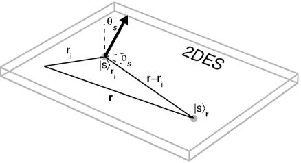
Figure 1: Schematic sketch of a 2DES, where an electron spin described by a given state ket $\left|s\right\rangle_{\vec{r}_{i}}$ is ideally injected at $\vec{r}_{i}$ with polar and azimuthal angles $\theta_{s}$ and $\phi_{s}$, respectively.

Specifically, how the given state ket $\left|s\right\rangle_{\vec{r}_{i}}$ after being spatially translated from $\vec{r}_{i}$ to $\vec{r}$ is simply obtained by operating on it with the translation operator $\mathcal{T}\left(\vec{a}\right)\equiv\exp\left(-i\vec{p}\cdot\vec{a}/\hbar\right)$: $\left|s\right\rangle_{\vec{r}}=\left|s\right\rangle_{\vec{r}_{i}\rightarrow\vec{r}}=\mathcal{T}\left(\vec{r}_{i}-\vec{r}\right)\left|s\right\rangle_{\vec{r}_{i}}$. Note that here we have assumed ideal point injection of spin. If the spins are injected via a finite-size contact, we have to sum over all the states coming from all the possible injection points:MHL2 $\left|s\right\rangle_{\vec{r}}\propto\sum_{i}\left|s\right\rangle_{\vec{r}_{i}\rightarrow\vec{r}}$. In general, for spin-orbit-coupled 2DESs we can obtain two spin-dependent eigenstates $|\sigma,\vec{k}_{\sigma}\rangle$, where $\sigma=\uparrow$ or $\downarrow$ is the index of the spin state subject to the wave vector $\vec{k}_{\sigma}$, and then expand the injected state ket using this basis: $\left|s\right\rangle_{\vec{r}_{i}}=\sum_{\sigma=\uparrow,\downarrow}|\sigma,\vec{k}_{\sigma}\rangle\langle\sigma,\vec{k}_{\sigma}|s\rangle_{\vec{r}_{i}}$. Operation of $\exp\left(-i\vec{p}\cdot\vec{a}/\hbar\right)$ on $\left|s\right\rangle_{\vec{r}_{i}}$ immediately gives different phases to the two components since $\exp\left(-i\vec{p}\cdot\vec{a}/\hbar\right)|\sigma,\vec{k}_{\sigma}\rangle=\exp(-i\vec{k}_{\sigma}\cdot\vec{a})|\sigma,\vec{k}_{\sigma}\rangle$ with $\left|k_{\uparrow}\right|\neq\left|k_{\downarrow}\right|$ in general. Such a phase difference, in fact, plays a key role in the spatial spin precession.

Next we will use the above strategy to solve two concrete examples: the RD [001] and the Dresselhaus [110] QWs.

II.2 PSH in RD [001] QWs

In this case we consider a [001]-grown 2DES confined in an asymmetric QW (where the Rashba effectRashba term exists) made of III-V semiconductors (where the Dresselhaus couplingDresselhaus term exists). Using the linear Rashba and the linear Dresselhaus model, the Hamiltonian can be written as

$$\mathcal{H}_{\left[001\right]}=\frac{p_{x}^{2}+p_{y}^{2}}{2m^{\star}}+\frac{\alpha}{\hbar}\left(p_{y}\sigma_{x}-p_{x}\sigma_{y}\right)+\frac{\beta}{\hbar}\left(p_{x}\sigma_{x}-p_{y}\sigma_{y}\right),$$ (1)

where $\alpha$ and $\beta$, assumed to be constant at present, are the Rashba and Dresselhaus strengths, respectively, and $m^{\star}$ is the electron effective mass. The well-known eigenfunctions are

$$\langle\vec{r}|\uparrow\downarrow,\vec{k}_{\uparrow\downarrow}\rangle=\frac{e^{i\vec{k}_{\uparrow\downarrow}\cdot\vec{r}}}{\sqrt{2}}\left(\begin{array}[c]{c}ie^{-i\varphi}\\ \pm 1\end{array}\right),$$ (2)

corresponding to the eigenenergies

$$E_{\uparrow\downarrow}(\vec{k})=\frac{\hbar^{2}k^{2}}{2m^{\star}}\pm\zeta\left(\alpha,\beta,\phi\right)k.$$ (3)

Here we have defined

$$\varphi\equiv\arg\left[\alpha\cos\phi+\beta\sin\phi+i(\alpha\sin\phi+\beta\cos\phi)\right]$$ (4)

and

$$\zeta\left(\alpha,\beta,\phi\right)=\sqrt{\alpha^{2}+\beta^{2}+2\alpha\beta\sin 2\phi},$$ (5)

where $\phi$ is the argument angle of $\vec{k}\equiv\left(k_{x},k_{y}\right)=k\left(\cos\phi,\sin\phi\right)$. Using the formalism introduced in Sec. II.1 and assuming that the spin is injected at $\vec{r}_{i}=\left(0,0\right)$, the spin vector formula, which had been previously derived,MHL reads

$$\left\langle\vec{\sigma}\right\rangle_{\vec{r}}^{\text{001}}=\left(\begin{array}[c]{c}-\cos\theta_{s}\cos\varphi\sin\Delta\theta_{\vec{r}}+\sin\theta_{s}\left(\cos\phi_{s}\cos^{2}\dfrac{\Delta\theta_{\vec{r}}}{2}-\cos\left(2\varphi-\phi_{s}\right)\sin^{2}\dfrac{\Delta\theta_{\vec{r}}}{2}\right)\\ -\cos\theta_{s}\sin\varphi\sin\Delta\theta_{\vec{r}}+\sin\theta_{s}\left(\sin\phi_{s}\cos^{2}\dfrac{\Delta\theta_{\vec{r}}}{2}-\sin\left(2\varphi-\phi_{s}\right)\sin^{2}\dfrac{\Delta\theta_{\vec{r}}}{2}\right)\\ \cos\theta_{s}\cos\Delta\theta_{\vec{r}}+\sin\theta_{s}\cos\left(\varphi-\phi_{s}\right)\sin\Delta\theta_{\vec{r}}\end{array}\right),$$ (6)

where

$$\Delta\theta_{\vec{r}}\equiv\frac{2m^{\star}\zeta\left(\alpha,\beta,\phi\right)r}{\hbar^{2}}$$ (7)

is the spin precession angle. Note that the position dependence of Eq. (6) lies in $\varphi$ and $\Delta\theta_{\vec{r}}$. Now we apply the condition $\alpha=\beta$ to fit the ReD condition. Obviously, we obtain $\varphi\left(\alpha=\beta\right)=\pi/4$ and $\zeta\left(\alpha,\alpha,\phi\right)=2\alpha\cos\left(\pi/4-\phi\right)$, leading to the precession angle

$$\Delta\theta_{\vec{r}}=\frac{4m^{\star}\alpha}{\hbar^{2}}r_{110}\equiv\Delta\theta_{\text{RD}}$$ (8)

with $r_{110}\equiv r\cos\left(\pi/4-\phi\right)$. It turns out that the position dependence of the spin vector is now reduced to only $\Delta\theta_{\vec{r}}$ through Eq. (8), which depends only on the net displacement in the [110] direction. Thus our previous results had indeed implied the PSH proposed by Bernevig et al.PSH

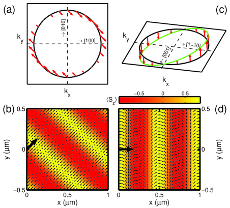
Figure 2: (Color online) Effective magnetic fields drawn in the $k_{x}$-$k_{y}$ coordinates for (a) the RD model, and (c) the Dresselhaus [110] model. (b) and (d) show the corresponding PSH patterns in a $1\times 1$ $\operatorname{\mu m}^{2}$ InAs-based 2DES, with assumed point injection of spins indicated by the bold arrows. Color bar calibrates $\left\langle S_{z}\right\rangle$ in (b) and $\left\langle S_{x}\right\rangle$ in (d), in units of $\hbar/2$, with yellow (bright) and red (dark) colors meaning positive and negative values, respectively.

In fact, in the RD condition the effective magnetic field generated by the Rashba and Dresselhaus spin-orbit couplings can be depicted in the momentum space as shown in Fig. 2(a), where the field directions are constant (pointing to either [11̄0] or [1̄10]) while the field strength depends on the projection of $k$ on [110] direction. This can be seen by defining the spin-orbit (effective magnetic) field as $\vec{B}_{\text{eff}}\equiv\zeta\langle\uparrow,\vec{k}_{\uparrow}|\vec{\sigma}|\uparrow,\vec{k}_{\uparrow}\rangle$, so that with the RD condition we have

$$\vec{B}_{\text{RD}}=\sqrt{2}\alpha\cos\left(\dfrac{\pi}{4}-\phi\right)\left(1,-1,0\right)\text{ .}$$ (9)

Now, we consider a $1\times 1$ $\operatorname{\mu m}^{2}$ InAs-based 2DES and apply Eq. (6) with $\alpha=\beta$ to obtain the PSH. Inside the 2DES, $m^{\star}=0.023m_{0}$, $m_{0}$ being the electron rest mass, and the Dresselhaus coupling strength is put at $\beta=1.062\times 10^{-2}$ $\operatorname{eV}\operatorname{nm}$ to simulate a 5-$\operatorname{nm}$-thick InAs quantum well.Knap As shown in Fig. 2(b), we have obtained the PSH in agreement with the prediction of Bernevig et al., in a more concrete way. Note that here we have assumed a point spin injection at $\left(x=0,y=0\right)$ with spin polarization parallel to [110].

II.3 PSH in Dresselhaus [110] QWs

Next we consider the Dresselhaus [110] model, where the 2DES is grown along [110] and is described by the Hamiltonian

$$\mathcal{H}_{\left[110\right]}=\frac{p_{x}^{2}+p_{y}^{2}}{2m}-2\frac{\beta}{\hbar}p_{x}\sigma_{z},$$ (10)

which is in a diagonal form. The eigenfuntions are

$$\left\langle\vec{r}|\uparrow,k_{\uparrow}\right\rangle=e^{i\vec{k}_{\uparrow}\cdot\vec{r}}\left|\uparrow\right\rangle\doteq e^{i\vec{k}_{\uparrow}\cdot\vec{r}}\left(\begin{array}[c]{c}1\\ 0\end{array}\right)$$ (11)

and

$$\left\langle\vec{r}|\downarrow,k_{\downarrow}\right\rangle=e^{i\vec{k}_{\downarrow}\cdot\vec{r}}\left|\downarrow\right\rangle\doteq e^{i\vec{k}_{\downarrow}\cdot\vec{r}}\left(\begin{array}[c]{c}0\\ 1\end{array}\right),$$ (12)

corresponding to the eigenenergies

$$E_{\uparrow\downarrow}(\vec{k})=\frac{\hbar^{2}k^{2}}{2m^{\star}}\mp 2\beta k_{x}.$$ (13)

Using the formalism introduced in Sec. II.1, we obtain the spatially evolved state ket

$$\left|s\right\rangle_{\vec{r}_{i}\rightarrow\vec{r}}=\sum_{\sigma=\uparrow,\downarrow}\exp\left(-\frac{i\Delta\theta_{\text{110}}}{2}\right)c_{\sigma}\left|\sigma\right\rangle,$$ (14)

with the phase

$$\Delta\theta_{\text{110}}=\left(k_{\downarrow}-k_{\uparrow}\right)r=\frac{4m^{\star}\beta}{\hbar^{2}}r_{\text{1\={1}0}},$$ (15)

where $c_{\sigma}=\left\langle\sigma|s\right\rangle_{\vec{r}_{i}}$ are the expansion coefficients and $r_{\text{1\={1}0}}\equiv r\cos\phi$ is the displacement along the $\phi=0$ direction. Note that in this Dresselhaus [110] model, the $x$ direction ($\phi=0$) is parallel with [11̄0]. As in the RD case, the precession angle depends on the net displacement along [11̄0].

Applying Eq. (14) with expansion coefficients $c_{\uparrow}=e^{-i\phi_{s}}\cos\left(\theta_{s}/2\right)$ and $c_{\downarrow}=\sin\left(\theta_{s}/2\right)$, we obtain the spin vector formula for the Dresselhaus [110] model:

$$\left\langle\vec{\sigma}\right\rangle_{\vec{r}}^{\text{110}}=\left(\begin{array}[c]{c}\sin\theta_{s}\left(\cos\phi_{s}\cos\Delta\theta_{\text{110}}-\sin\phi_{s}\sin\Delta\theta_{\text{110}}\right)\\ -\sin\theta_{s}\left(\cos\phi_{s}\sin\Delta\theta_{\text{110}}+\sin\phi_{s}\cos\Delta\theta_{\text{110}}\right)\\ \cos\theta_{s}\end{array}\right).$$ (16)

Comparing Eqs. (13) with (3), the spin splitting linear in $k$ in this Dresselhaus [110] case is $2\beta k_{x}=\left(2\beta\cos\phi\right)k$, so we can define

$$\vec{B}_{\text{110}}\equiv 2\beta\cos\phi\left\langle\uparrow\right|\vec{\sigma}\left|\uparrow\right\rangle=2\beta k\cos\phi\left(0,0,1\right)$$ (17)

to depict the effective magnetic field in the $k$ space, as shown in Fig. 2(c). Correspondingly, the PSH pattern is drawn in Fig. 2(d), where the same material parameters (including the Dresselhaus strength) as in Fig. 2(b) are taken (except that there is no $\alpha$ here), and an $x$-polarized spin is injected at $\left(0,0\right)$.

II.4 More on the spin precession: Space translation vs. time evolution

Before we move on to the influence on the PSH due to the random Rashba effect, below we provide a series of discussion over the time evolution of spin in these spin-orbit coupled systems. So far, the above position-dependent spin vectors are based on the time-independent Schrödinger approach. In fact, the key to such space-resolved spin precession lies in the assumption of $E_{\uparrow}=E_{\downarrow}=E_{F}$, $E_{F}$ being the Fermi energy. Under this assumption, the injected spin is projected onto two available states at the Fermi level with equal energy but different momentums (see the “horizontal projection” in Fig. 3). The difference in the projected wave vectors, as we mentioned in Sec. II.1, leads to a phase difference between the two spin components of the total wave function when spatially translated by a distance, and an angle of rotation of the spin then occurs. Meanwhile, with $E_{\uparrow}=E_{\downarrow}$ the wave function does not have nontrivial time dependence since the time evolution operator $\exp\left(-i\mathcal{H}t/\hbar\right)$ produces equal phases for both spin components. In other words, the persistence for the spin precession pattern, or the PSH, is merely a built-in property, once the projected states satisfy $E_{\uparrow}=E_{\downarrow}$.

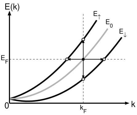
Figure 3: Band structure of a spin-orbit coupled 2DES. Vertical projection fixes $k$ as $k_{F}$, leading to time-resolved spin precession, while horizontal projection fixes energy as $E_{F}$, leading to spatial spin precession.

From the quantum-mechanical viewpoint, it is only when the injected electron is projected onto states with $E_{\uparrow}\neq E_{\downarrow}$ that leads to nontrivial time dependence. If we regard the spin-orbit interaction as an effective magnetic field $\vec{B}_{\text{eff}}$ and treat the injected electron spin as a constantly moving particle with wave vector $k_{F}$ in the 2DES, the sudden turn-on of $\vec{B}_{\text{eff}}$ splits the energy level the electron originally occupies, leaving the momentum it carries unchanged. See the “vertical projection” in Fig. 3. Taking the Rashba-Dresselhaus [001] 2DES for example (not necessarily RD), the split levels are indicated in Eq. (3), or simply $E_{0}\pm\Delta E$ with $\Delta E=\zeta\left(\alpha,\beta,\phi\right)k$ and $E_{0}=\hbar^{2}k^{2}/2m^{\star}$. It turns out that different phases $\exp\left(\mp i\Delta Et/\hbar\right)$ for the two spin components will emerge, under the operation of $\exp\left(-i\mathcal{H}t/\hbar\right)$. Thus we can analogously use the ket $\left|s\right\rangle_{t}=e^{iE_{0}t/\hbar}(c_{\uparrow}e^{-i\Delta\theta_{t}/2}|\uparrow,\vec{k}_{\uparrow}\rangle+c_{\downarrow}e^{i\Delta\theta_{t}/2}|\downarrow,\vec{k}_{\downarrow}\rangle)$ to derive the time-resolved spin-vector formulas, which are exactly of the same forms with the spatial ones, except that $\Delta\theta_{\vec{r}}$ is replaced by $\Delta\theta_{t}=2\zeta kt/\hbar$.

Quite interestingly, both methods (space translation and time evolution) lead to exactly the same precession angle, if we treat the electron as a moving particle with group velocity $v_{g}=\hbar k/m^{\star}$. For example, in the spatial treatment for the Rashba-Dresselhaus [001] QWs, the spin precession angle between two points $L$ apart is $\Delta\theta_{\vec{r}}=2m^{\star}\zeta L/\hbar^{2}$, while in the time treatment we have $\Delta\theta_{t}=2\zeta kL/v_{g}\hbar$, such that $\Delta\theta_{\vec{r}}=\Delta\theta_{t}$ is guaranteed. For a fixed propagation direction, the precession angle between any pair of injection-detection points depends only on the distance, but not the velocity (or the wave vector) of the electron. This is similar to a rolling disk without going into a slide in classical physics. In fact, these two ideal assumptions (horizontal and vertical projections shown in Fig. 3) are often adopted, although in real situations combined effects are more likely to occur. The actual projection of states may depend on the temperature fluctuation, interaction between the injected electrons and the 2DES, and even the applied bias. These may require further studies but we end the discussion here.

Finally, it is of much pedagogical meaning to relate the Schrödinger and the Heisenberg formalisms for the time evolution of spin in the Rashba-Dresselhaus problems. If we fix the electron momentum as $\hbar k$ (the vertical projection), from the Hamiltonian for, e.g., the Rashba-Dresselhaus [001] general case shown in Eq. (1) we can solve the time dependence of the spin operators in the Heisenberg picture. Note that here we treat $p=\hbar k$ in Eq. (1) simply as numbers. Only the $\sigma$’s therein are operators. Using the Heisenberg equation of motion $i\hbar\dot{\sigma}_{i}=\left[\sigma_{i},\mathcal{H}\right]$, one can obtain the differential equations governing the time evolution of the spin components: $\dot{\sigma}_{x}=a\sigma_{z},$ $\dot{\sigma}_{y}=b\sigma_{z},$ and $\dot{\sigma}_{z}=-a\sigma_{x}-b\sigma_{y}$, with $a\equiv 2\left(\alpha k_{x}+\beta k_{y}\right)/\hbar$ and $b\equiv 2\left(\alpha k_{y}+\beta k_{x}\right)/\hbar$. These differential equations can be easily solved to obtain

$$\left\langle\sigma_{x}\right\rangle_{t} =\left[\left\langle\sigma_{z}\right\rangle_{0}\sin\omega t-\left(\left\langle\sigma_{x}\right\rangle_{0}\cos\varphi+\sigma_{y}^{0}\sin\varphi\right)\right.$$

$$\times\left.\left(1-\cos\omega t\right)\right]\cos\varphi+\left\langle\sigma_{x}\right\rangle_{0}$$ (18a)

$$\left\langle\sigma_{y}\right\rangle_{t} =\left[\left\langle\sigma_{z}\right\rangle_{0}\sin\omega t-\left(\left\langle\sigma_{x}\right\rangle_{0}\cos\varphi+\left\langle\sigma_{y}\right\rangle_{0}\sin\varphi\right)\right.$$

$$\times\left.\left(1-\cos\omega t\right)\right]\sin\varphi+\left\langle\sigma_{y}\right\rangle_{0}$$ (18b)

$$\left\langle\sigma_{z}\right\rangle_{t} =\left\langle\sigma_{z}\right\rangle_{0}\cos\omega t-\left(\left\langle\sigma_{x}\right\rangle_{0}\cos\varphi+\left\langle\sigma_{y}\right\rangle_{0}\sin\varphi\right)$$

$$\times\sin\omega t$$ (18c)

with $$\omega^{2}\equiv a^{2}+b^{2} \left\langle\sigma_{i}\right\rangle_{0}\equiv\left\langle\sigma_{i}\right\rangle_{t=0} \left\langle\sigma_{x}\right\rangle_{0}=\sin\theta_{s}\cos\phi_{s}, \left\langle\sigma_{y}\right\rangle_{0}=\sin\theta_{s}\sin\phi_{s} \left\langle\sigma_{z}\right\rangle_{0}=\cos\theta_{s} \theta_{s} \phi_{s} \Delta\theta_{\vec{r}} \omega t$$ and . Setting the initial conditions as , , i.e., the injected spin with polar and azimuthal angles and , respectively (see Fig. 1), one can prove that Eqs. (18a)–(18c) are equivalent to Eq. (6) with replaced by .

II.5 Random Rashba effect on the PSH in RD [001] QWs

Now we go back to the PSH and focus on the RD [001] case. Whereas the Rashba spin-orbit coupling partly stems from the Coulomb field generated from the ionized dopants in the vicinity of the 2DES layer (usually some tens of nanometers apart), the Rashba parameter is actually position dependent. Usually, these dopants are randomly distributed (depending on the doping techniques), and the resulting Rashba field may be constant in average but fluctuating locally in nanometer scales (depending on the dopant concentration). With this position dependence of $\alpha$, the Rashba term previously written as $\mathcal{H}_{R}=\left(\alpha/\hbar\right)\left(p_{y}\sigma_{x}-p_{x}\sigma_{y}\right)$ in Eq. (1) has to be symmetrized as

$$\mathcal{H}_{R}=\frac{1}{2\hbar}\left[\alpha\left(\vec{r}\right)\left(p_{y}\sigma_{x}-p_{x}\sigma_{y}\right)+\left(p_{y}\sigma_{x}-p_{x}\sigma_{y}\right)\alpha\left(\vec{r}\right)\right],$$ (19)

since $\alpha\left(\vec{r}\right)$ in general no longer commutes with $p_{x}$ or $p_{y}$. In this case, the full Hamiltonian is not easy to diagonolize, and the desired eigenfunctions serving as the basis to expand the injected spin state are not accessible. However, a convenient way of contour-integral method can be applied to directly obtain the spatially evolved state ket subject to the injected electron spin, without finding the basis for the entire system.nonuniform Thus spin vectors in such nonuniform Rashba-Dresselhaus 2DESs turn out to be still computable with, however, the precession angle given by a contour-integral form

$$\Delta\Theta=\frac{2}{\hbar^{2}}\int_{C}m^{\star}\zeta\left(\alpha\left(\vec{r}\right),\beta,\phi\right)d\vec{\ell},$$ (20)

where $C$ is the path the spin goes through [cf. Eq. (7) for the constant Rashba model]. Note that in Eq. (20), $\phi$ is the argument angle of $d\vec{\ell}$ along the tangential direction at position $\vec{r}$ on the path $C$, which is taken as the straight line connecting the injection and detection points in the following numerical calculations.

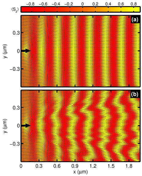
Figure 4: (Color online) PSH patterns in RD [001] QWs with (a) regularly and (b) randomly distributed dopants. Bold arrows indicate the assumed point injection of spin. Color bar calibrates $\left\langle S_{z}\right\rangle$ in units of $\hbar/2$ with yellow (bright) and red (dark) colors meaning positive and negative values, respectively. Note that the $x$ axis here is pointing to [110].

To investigate the influence on the PSH due to such a random Rashba effect, let us consider two $2.0\times 1.2$ $\operatorname{\mu m}^{2}$ InAs-based 2DESs, one with regular dopant distribution and the other with random distribution. Note that, in the latter case, the coordinate of each dopant is completely random: probability of each dopant to occupy each available lattice site is equally likely. Detailed process of generating the position dependent Rashba parameter $\alpha\left(\vec{r}\right)$ can be found in Refs. Sherman, and nonuniform, . The dopant concentration is fixed at $\bar{n}=2.5\times 10^{11}$ $\operatorname{cm}^{-2}$, leading to the average Rashba field $\left\langle\alpha\right\rangle\approx 0.019$ $\operatorname{eV}\operatorname{nm}$. We put $\beta=\left\langle\alpha\right\rangle$, corresponding to the QW thickness of around 3.7 $\operatorname{nm}$, to simulate the RD condition. Applying the contour-integral method of our recent work,nonuniform we plot the PSH patterns for the regular and the random cases in Figs. 4(a) and 4(b), respectively. Note that the plots here have been rotated so that the $x$ axis is parallel with [110] {instead of [100] in the previous demonstration of Fig. 2(b)}.

Clearly, in the regular case, even though the Rashba parameter is not constant in space (spatial profile may be seen in Ref. nonuniform, ), the PSH pattern is still almost perfect, compared to the one predicted in the calculation with the constant Rashba model. When the dopants are randomly distributed, Fig. 4(b) shows a distorted PSH pattern, which may imply an intrinsic difficulty in experimental observation of the PSH in RD [001] QWs. In addition, since the distortion actually stems from the difference in $\Delta\Theta$ given in Eq. (20) along different injection-detection paths, the distortion effect may grow with distance. Indeed, one can see that the farther stripes in Fig. 4(b) are more distorted than the nearer ones. Note that here we have assumed these two somewhat wide channels to be ballistic and unbounded, so that the distortion effect is completely induced by the random Rashba effect.

Alternatively, the difference in $\Delta\Theta$ for different paths may accumulate faster by raising the composite spin-orbit coupling strength $\zeta$, or the Rashba strength $\alpha$, which increases with the dopant concentration $\bar{n}$. When putting a higher $\bar{n}$, the stronger Rashba strength creates a PSH pattern with more stripes, among which the farther (nearer) ones will be more (less) distorted. In this case the distorted pattern is similar to the one we have shown in Fig. 4(b), except that only a shorter channel is required, and we do not further show here.

III Conclusion

To conclude, we have presented refined PSH patterns in RD [001] and the Dresselhaus [110] QWs, first predicted by Bernevig et al.PSH For the RD [001] case, we have shown that the PSH had actually been implied in our previous results.MHL ; MHL2 For the Dresselhaus [110] case, we have also derived the spin-vector formula using the same method. For both cases, we have shown the most important feature of the PSH: the spin precession angle depends only on the net displacement of the injected spin along certain directions ($\pm[110]$ for the RD [001] and $\pm[1\bar{1}0]$ for the Dresselhaus [110] cases), and hence the name “helix.” This special feature guarantees the probability of experimentally observing the PSH since the spin direction does not depend on the incoming direction: momentum scattering is even allowed.

We have also discussed the time evolution of spin in the Rashba-Dresselhaus problem. In the quantum-mechanical interpretation, the persistence of the PSH seems to be inherent in any systems, not necessarily the RD [001] or the Dresselhaus [110] QW, once the injected spin is projected onto states with equal energy (the ”horizontal projection” sketched in Fig. 3). Meanwhile, when treating the electron as a constantly moving particle with the group velocity $\hbar k/m^{\star}$, the other assumption of vertical projection will lead to the same physics, i.e., the spin direction at a certain position in the 2DES does not depend on time.

Applying the contour-integral method,nonuniform we have also examined the influence on the PSH pattern due to the random Rashba effect for the RD [001] case. The obtained results show that unless the dopants are regularly distributed, the PSH pattern may be distorted (though not totally destroyed) by the random effect. In addition, the distortion effect is observed to grow with longer channel length or higher dopant concentration (stronger Rashba strength). Therefore, symmetric QWs grown along [110] with only the Dresselhaus coupling may be a better candidate to observe the predicted PSH.

Finally, we remind here that in this Dresselhaus [110] model, the PSH period given by $\pi\hbar^{2}/4m^{\star}\beta$ is quite sensitive to the electron effective mass. For example, GaAs and InAs have similar bulk Dresselhaus coefficients,Winkler ; Knap but a significant difference in the two-dimensional electron effective mass.book With $m_{\text{GaAs}}^{\star}/m_{\text{InAs}}^{\star}\approx 3$, the PSH pattern size using GaAs QWs will be about three times smaller than for InAs QWs, and will therefore require experimental setups with higher resolution.

- (1) R. Winkler, Spin-Orbit Coupling Effects in Two-Dimensional Electron and Hole Systems (Springer, Berlin, 2003).
- (2) Ming-Hao Liu, Ching-Ray Chang, and Son-Hsien Chen, Phys. Rev. B 71, 153305 (2005); Ming-Hao Liu and Ching-Ray Chang, J. Magn. Magn. Mater. 304, 97 (2006).
- (3) Ming-Hao Liu and Ching-Ray Chang, Phys. Rev. B 73, 205301 (2006).
- (4) Igor Žutić, Jaroslav Fabian, and S. Das Sarma, Rev. Mod. Phys. 76, 323 (2004).
- (5) S. Datta and B. Das, Appl. Phys. Lett. 56, 665 (1990).
- (6) Semiconductor Spintronics and Quantum Computation, edited by D. D. Awschalom, D. Loss, and N. Samarth (Springer, Berlin, 2002).
- (7) J. Schliemann, J. C. Egues, and D. Loss, Phys. Rev. Lett. 90, 146801 (2003).
- (8) M. I. Dyakonov and V. I. Perel’, Zh. Eksp. Teor. Fiz. 60, 1954 (1971) [Sov. Phys. JETP 33, 1053 (1971)]; Fiz. Tverd. Tela (Leningrad) 13, 3581 (1971) [Sov. Phys. Solid State 13, 3023 (1972)].
- (9) Y. Ohno, R. Terauchi, T. Adachi, F. Matsukura, and H. Ohno, Phys. Rev. Lett. 83, 4196 (1999); K. C. Hall, K. Gündoğdu, E. Altunkaya, W. H. Lau, Michael E. Flatté, and Thomas F. Boggess, Phys. Rev B 68, 115311 (2003); S. Döhrmann, D. Hägele, J. Rudolph, M. Bichler, D. Schuh, and M. Oestreich, Phys. Rev. Lett. 93, 147405 (2004); A. W. Holleitner, V. Sih, R. C. Myers, A. C. Gossard, and D. D. Awschalom, Phys. Rev. Lett. 97, 036805 (2006).
- (10) B. Andrei Bernevig, J. Orenstein, and Shou-Cheng Zhang, Phys. Rev. Lett. 97, 236601 (2006).
- (11) E. Ya. Sherman, Appl. Phys. Lett. 82, 209 (2003); E. Ya. Sherman, Phys. Rev. B 67, 161303(R) (2003); E. Ya. Sherman and Jairo Sinova, Phys. Rev. B 72, 075318 (2005).
- (12) E. I. Rashba, Sov. Phys. Solid State 2, 1109 (1960); Yu. A. Bychkov and E. I. Rashba, JETP Lett. 39, 78 (1984).
- (13) G. Dresselhaus, Phys. Rev. 100, 580 (1955).
- (14) W. Knap, C. Skierbiszewski, A. Zduniak, E. Litwin-Staszewska, D. Bertho, F. Kobbi, J. L. Robert, G. E. Pikus, F. G. Pikus, S. V. Iordanskii, V. Mosser, K. Zekentes, and Yu. B. Lyanda-Geller, Phys. Rev. B 53, 3912 (1996).
- (15) Ming-Hao Liu and Ching-Ray Chang, Phys. Rev. B 74, 195314 (2006).
- (16) John H. Davies, The Physics of Low-Dimensional Semiconductors (Cambridge University Press, Cambridge, U.K., 1998).