Ion and polymer dynamics in polymer electrolytes PPO-LiClO₄:
II. ²H and ⁷Li NMR stimulated-echo experiments

Abstract

We use ²H NMR stimulated-echo spectroscopy to measure two-time correlation functions characterizing the polymer segmental motion in polymer electrolytes PPO-LiClO₄ near the glass transition temperature $T_{g}$. To investigate effects of the salt on the polymer dynamics, we compare results for different ether oxygen to lithium ratios, namely, 6:1, 15:1, 30:1 and $\infty$. For all compositions, we find nonexponential correlation functions, which can be described by a Kohlrausch function. The mean correlation times show quantitatively that an increase of the salt concentration results in a strong slowing down of the segmental motion. Consistently, for the high 6:1 salt concentration, a high apparent activation energy $E_{a}\!=\!4.1\mathrm{\,eV}$ characterizes the temperature dependence of the mean correlation times at $T_{g}\!<\!T\!\lesssim\!1.1\,T_{g}$, while smaller values $E_{a}\!\approx\!2.5\mathrm{\,eV}$ are observed for moderate salt contents. The correlation functions are most nonexponential for 15:1 PPO-LiClO₄, whereas the stretching is reduced for higher and lower salt concentrations. This finding implies that the local environments of the polymer segments are most diverse for intermediate salt contents, and, hence, the spatial distribution of the salt is most heterogeneous. To study the mechanisms of the segmental reorientation, we exploit that the angular resolution of ²H NMR stimulated-echo experiments depends on the length of the evolution time $t_{p}$. A similar dependence of the correlation functions on the value of $t_{p}$ in the presence and in the absence of ions indicates that addition of salt hardly affects the reorientational mechanism. For all compositions, mean jump angles of about 15^∘ characterize the segmental reorientation. In addition, comparison of results from ²H and ⁷Li NMR stimulated-echo experiments suggests a coupling of ion and polymer dynamics in 15:1 PPO-LiClO₄.

I Introduction

The glass transition of polymer melts is of tremendous interest from the viewpoints of fundamental and applied science. This importance triggered a huge amount of studies, which established that the glass transition phenomenon of polymers is related to the $\alpha$ process.McCrum ; Ferry ; Spiess An improvement of our understanding of the glass transition thus requires detailed characterization of the microscopic dynamics underlying the $\alpha$ process. In particular, it is important to determine both the time scale and the geometry of the molecular dynamics.

Various methods were used to measure the correlation time of the $\alpha$ process, $\tau_{\alpha}$. For polymers, a striking feature of the $\alpha$ process is a non-Arrhenius temperature dependence. In most cases, the Vogel-Fulcher-Tammann equation, $\tau_{\alpha}(T)\!=\!\tau_{0}\exp\left[B/(T\!-\!T_{0})\right]$, enables a satisfactory interpolation of the data, suggesting a divergence of the correlation time at a temperature $T_{0}$ not too far below the glass transition temperature $T_{g}$, i.e., $T_{0}\!\approx\!T_{g}\!-\!50\mathrm{\,K}$.Spiess Hence, high apparent activation energies $E_{a}$ characterize the temperature dependence of the $\alpha$ process close to $T_{g}$.Spiess Another intriguing property of the $\alpha$ process is a nonexponential loss of correlation, which is often well described by the Kohlrausch-Williams-Watts (KWW) function, $\exp[-(t/\tau)^{\beta}]$. By contrast, few experimental techniques yield detailed insights into the geometry of the molecular motion associated with the $\alpha$ process.

2D NMR provides straightforward access to both the time scale and the geometry of molecular reorientation in polymeric and molecular glass-forming liquids.Spiess ; Roessler ; Boehmer ; Duer ; Reichert 2D NMR experiments can be performed in the frequency domainWefing ; Kaufmann ; Pschorn ; Schaefer and in the time domain.SpiessTD ; Diehl ; RoEi ; Geil ; Hinze ; BoHi ; Tracht The latter approach is also called stimulated-echo (SE) spectroscopy. Concerning the geometry of polymer dynamics, 2D NMR studies ruled out the existence of well-defined jump angles $\gamma$ for the rotational jumps associated with the $\alpha$ process.Spiess ; Boehmer ; Reichert ; Wefing ; Kaufmann ; Pschorn ; Schaefer ; Tracht Instead, results from 2D and 3D NMR showed that the reorientation is comprised of rotational jumps about angles $\gamma\!=\!10\!-\!40^{\circ}$ between which the polymer segments show isotropic rotational diffusion.Schaefer ; Tracht ; Leisen ; Heuer ; Kuebler

We carry out ²H NMR SE experiments to investigate the segmental motion of poly(propylene oxide) (PPO) containing various amounts of the salt LiClO₄. Thus, we focus on polymer electrolytes, which are promising candidates for applications in energy technologies.Gray Since the use of polymer electrolytes is still limited by the achievable electric conductivities, there is considerable interest to speed up the ionic diffusion. It has been established that segmental motion of the host polymer facilitates the ionic migration,Armand ; Ratner yet the understanding of this coupling is incomplete. In dielectric spectroscopy, the ionic diffusion coefficient and the relaxation rate of polymer segments in contact with salt were found to show a linear relationship,Furukawa suggesting that segmental motion triggers the elementary steps of the charge transport.

Polymer electrolytes PPO-LiClO₄ have attracted much attention because of high ionic conductivities together with their amorphous nature.Armand When studied as a function of the salt concentration, the electric conductivity $\sigma_{dc}$ at room temperature shows a broad maximum at ether oxygen to lithium ratios, O:Li, ranging from about 10:1 to 30:1.Furukawa ; McLin For such intermediate salt concentrations, differential scanning calorimetry showed the existence of two glass transition steps,Moacanin ; Vachon_1 ; Vachon_2 implying a liquid-liquid phase separation into salt-rich and salt-depleted regions. An inhomogeneous structure was also assumed to explain results from dielectric and photon correlation spectroscopies for intermediate salt concentrations,Furukawa ; Bergman which give evidence for the presence of two processes related to fast and slow polymer dynamics. By contrast, the existence of salt-rich and salt-depleted microphases was challenged in neutron scattering work on mixtures PPO-LiClO₄.Carlsson_1 ; Carlsson_2 Finally, it was proposed that a structure model of 16:1 PPO-LiClO₄ resulting from reverse Monte-Carlo simulations of diffraction data enables reconciliation of the apparent discrepancies.Carlsson_3 It does feature salt-rich and salt-depleted regions, but the structural heterogeneities occur on a small length scale of $\mathrm{1\,nm}$.

In NMR work on polymer electrolytes, the ion dynamics was studied in some detail,Roux ; Chung_1 ; Chung_2 ; Adamic ; Fan ; Donoso ; Forsyth e.g., ionic self diffusion coefficients were determined using field-gradient techniques,Vincent ; Arumugam ; Ward while investigations of the polymer dynamics were restricted to analysis of the spin-lattice relaxation.Ward ; Roux ; Donoso Only recently, modern NMR methods were employed to study the segmental motion in organic-inorganic hybrid electrolytes.Kao We use various ²H and ⁷Li NMR techniques for a detailed characterization of the polymer and the ion dynamics in polymer electrolytes PPO-LiClO₄. Our goals are twofold. From the viewpoint of fundamental science, we ascertain how the presence of salt affects the polymer dynamics. In this way, we tackle the question how structural heterogeneities introduced by the addition of salt affect the glass transition of polymers. From the viewpoint of applied science, we investigate how the polymer assists the ionic diffusion so as to give support to the development of new materials. For example, we compare ²H and ⁷Li NMR data to study the coupling of ion and polymer dynamics.

Very recently, we presented results from ²H and ⁷Li NMR line-shape analysis for polymer electrolytes PPO-LiClO₄.Vogel The ²H NMR spectra indicate that addition of salt slows down the segmental motion. Moreover, the line shape shows that broad distributions of correlation times $G(\log\tau)$ govern the polymer dynamics. These dynamical heterogeneities are particularly prominent for intermediate salt concentrations. While such line-shape analysis provides valuable insights on a qualitative level, the possibilities for a quantification are limited.

Here, we exploit that ²H NMR SE spectroscopy enables measurement of two-time correlation functions that provide quantitative information about polymer segmental motion on a microscopic level.Spiess In this way, we continue to investigate to which extent presence of salt affects the $\alpha$ process of polymer melts. While previous ²H NMR SE studies focussed on molecules featuring a single deuteron species, two deuteron species, which exhibit diverse spin-lattice relaxation (SLR) and spin-spin relaxtion (SSR), contribute to the correlation functions in our case. Therefore, it is necessary to ascertain the information content of this method in such situation. We will demonstrate that, in the presence of two deuteron species, it is necessary to use appropriate experimental parameters, when intending to correct the measured data for relaxation effects, which is highly desirable in order to extend the time window of the experiment.

II Theory

II.1 Basics of ²H and ⁷Li NMR

Solid-state ²H NMR probes the quadrupolar precession frequency $\omega_{Q}$, which is determined by the orientation of the quadrupolar coupling tensor with respect to the external static magnetic flux density $\mathbf{B_{0}}$. This tensor describes the interaction of the nuclear quadrupole moment with the electric field gradient at the nuclear site. The monomeric unit of the studied PPO, [CD₂-CD(CD₃)-O]_n, features three deuterons in the backbone and three deuterons in the methyl group, which will be denoted as B deuterons and M deuterons, respectively. For both deuteron species, the coupling tensor is approximately axially symmetric.Vogel Then, $\omega_{Q}$ is given bySpiess

$$\omega_{Q}(\theta)=\pm\frac{\delta_{y}}{2}\,(3\cos^{2}\theta_{y}-1)$$ (1)

Here, $y\!=\!B,M$ refers to the different deuteron species. For the B deuterons, $\theta_{B}$ specifies the angle between the axis of the C-D bond and $\mathbf{B_{0}}$ and the anisotropy parameter amounts to $\delta_{B}\!\approx\!2\pi\!\times\!\mathrm{120\,kHz}$.Vogel For the M deuterons, the coupling tensor is preaveraged due to fast threefold jumps of the methyl group at the studied temperatures. Consequently, $\theta_{M}$ is the angle between the threefold axis and $\mathbf{B_{0}}$ and the anisotropy parameter is reduced by a factor of three, $\delta_{M}\!=\!\delta_{B}/3$.Spiess The two signs in Eq. (1) correspond to the two allowed transitions between the three Zeeman levels of the $I\!=\!1$ nucleus. We see that, for both deuteron species, the quadrupolar precession frequency is intimately linked to the orientation of well defined structural units and, hence, segmental motion renders $\omega_{Q}$ time dependent, which is the basis of ²H NMR SE spectroscopy.Spiess ; Roessler

In solid-state ⁷Li NMR ($I\!=\!3/2$), the quadrupolar interaction affects the frequencies of the satellite transitions $\pm 3/2\!\leftrightarrow\!\pm 1/2$, while that of the central transition $1/2\!\leftrightarrow\!-1/2$ is unchanged. For polymer electrolytes, diverse lithium ionic environments lead to a variety of shapes of the quadrupolar coupling tensor so that ⁷Li NMR spectra exhibit an unstructured satellite component.Chung_1 ; Vogel Analysis of ⁷Li NMR SE experiments will be straightforward if the time dependence $\omega_{Q}(t)$ is solely due to lithium ionic motion. This condition is approximately met in applications on solid-state electrolytes, i.e., when the lithium ionic diffusion occurs in a static matrix.BoehmerLi_1 ; BoehmerLi_2 For polymer electrolytes, the lithium environments change due to ion and polymer dynamics, occurring on comparable time scales. Consequently, both these dynamic processes can render the electric field gradient at the nuclear site and, hence, $\omega_{Q}$ time dependent.Zax Thus, when ⁷Li NMR is used to investigate charge transport in polymer electrolytes, it is a priori not clear to which extent the lithium ionic diffusion and the rearrangement of the neighboring polymer chains are probed.

II.2 ²H NMR stimulated-echo spectroscopy

²H NMR SE spectroscopy proved a powerful tool to study molecular dynamics with correlation times in the range of $10\,\mathrm{\mu s}\!\leq\!\tau\!\leq\!1\mathrm{\,s}$.Boehmer ; SpiessTD ; Diehl ; RoEi ; Geil ; Hinze ; BoHi ; Fujara_1 ; Fujara_2 ; Vogel_1 ; Vogel_2 ; Jeffrey In this experiment, the frequency $\omega_{Q}$ is probed twice during two short evolution times $t_{p}\!\ll\tau$, which embed a long mixing time $t_{m}\!\approx\tau$. In detail, appropriate three-pulse sequences are used to generate a stimulated echo.Spiess ; Duer ; Roessler ; Boehmer ; Reichert Evaluating the height of this echo for various mixing times $t_{m}$ and constant evolution time $t_{p}$, it is possible to measure two-time correlation functions. Neglecting relaxation effects, one obtains depending on the pulse lengths and phases in the three-pulse sequenceSpiess ; Duer ; Roessler ; Boehmer ; Reichert

$$E_{2}^{SS}(t_{m};t_{p})=\langle\,\sin[\,\omega_{Q}(0)t_{p}]\cdot\sin[\,\omega_{Q}(t_{m})t_{p}]\,\rangle,$$ (2)

$$E_{2}^{CC}(t_{m};t_{p})=\langle\,\cos[\,\omega_{Q}(0)t_{p}]\cdot\cos[\,\omega_{Q}(t_{m})t_{p}]\,\rangle.$$ (3)

Here, the brackets $\langle\dots\rangle$ denote the ensemble average, including the powder average for our isotropic distribution of molecular orientations.34 We see that the frequencies $\omega_{Q}(0)$ and $\omega_{Q}(t_{m})$ are correlated via sine or cosine functions. In general, molecular reorientation during the mixing time leads to $\omega_{Q}(0)\!\neq\!\omega_{Q}(t_{m})$ and, hence, to decays of $E_{2}^{SS}(t_{m})$ and $E_{2}^{CC}(t_{m})$. Normalizing these correlation functions, we obtain ($x\!=\!SS,CC$)

$$F_{2}^{x}(t_{m};t_{p})=\frac{E_{2}^{x}(t_{m};t_{p})}{E_{2}^{x}(0;t_{p})}$$ (4)

to which we will refer as sin-sin and cos-cos correlation functions in the following.

The dependence of $F_{2}^{x}(t_{m};t_{p})$ on the evolution time provides access to the jump angles of molecular rotational jumps.Hinze ; BoHi ; Geil ; Tracht ; Jeffrey ; Vogel_1 ; Vogel_2 This approach exploits that the angular resolution of the experiment depends on the length of the evolution time $t_{p}$. When the quadrupolar coupling tensor is axially symmetric, the sin-sin correlation function for $t_{p}\!\rightarrow\!0$ yields the rotational correlation function of the second Legendre polynomial, $F_{2}(t_{m})$:

$$F_{2}^{SS}(t_{m};t_{p}\!\rightarrow\!0)\propto t_{p}^{2}\,\langle\,\omega_{Q}(0)\,\omega_{Q}(t_{m})\,\rangle\propto$$

$$\propto\langle P_{2}[\cos(\theta(0)]P_{2}[\cos(\theta(t_{m})]\rangle\propto F_{2}(t_{m}).$$ (5)

On extension of the evolution time, smaller and smaller changes of the resonance frequency, $|\omega_{Q}(t_{m})\!-\!\omega_{Q}(0)|$, are sufficient to observe a complete decay of $F_{2}^{x}(t_{m};t_{p})$, i.e., isotropic redistribution of the molecular orientations is no longer required. In the limit $t_{p}\!\rightarrow\!\infty$,

$$F_{2}^{x}(t_{m};t_{p}\!\rightarrow\!\infty)=\langle\delta[\,\omega_{Q}(t_{m})\!-\!\omega_{Q}(0)]\rangle\equiv F_{2}^{J}(t_{m})$$ (6)

and, hence, the jump correlation function $F_{2}^{J}(t_{m})$ is measured, which characterizes the elementary steps of the reorientation process. The mean jump angle $\gamma$ of the molecular rotational jumps can be determined by comparison of the correlation times $\tau_{C}$ and $\tau_{J}$ characterizing the decays of $F_{2}(t_{m})$ and $F_{2}^{J}(t_{m})$, respectively,Anderson

$$\frac{\tau_{J}}{\tau_{C}}=\frac{3}{2}\sin^{2}\gamma.$$ (7)

Analysis of the complete dependence of the correlation time on the evolution time, $\tau(t_{p})$, provides further information about the distribution of jump angles.Hinze ; BoHi ; Tracht

Here, the existence of two deuteron species complicates the analysis of sin-sin and cos-cos correlation functions. Thus, prior to a presentation of experimental results, it is important to determine the interpretation of these correlation functions in such situation. In the first step, we will continue to neglect relaxation effects and study consequences of the different anisotropy parameters $\delta_{B}\!=\!3\delta_{M}$. In the second step, we will investigate how the interpretation of the correlation functions is affected by the fact that the deuteron species exhibit different spin-lattice and spin-spin relaxation times, $T_{1}$ and $T_{2}$, respectively.

In the first step, the non-normalized correlation functions can be written as the following sum of contributions from the B and the M deuterons

$$E_{2}^{x}(t_{m};t_{p}) = \sum_{y}m_{y}e_{2,y}^{x}(t_{m};t_{p})$$

$$e_{2,y}^{x}(t_{m};t_{p}) \!=\! \left[a_{y}^{x}(t_{p})\!-\!z_{y}^{x}(t_{p})\right]\phi_{y}^{x}(t_{m};t_{p})\!+\!z_{y}^{x}(t_{p})\>\>\>\>\>$$ (8)

Here, we consider that $e_{2,y}^{x}(t_{m};t_{p})$ decays from an initial correlation $a_{y}^{x}(t_{p})$ to a residual correlation $z_{y}^{x}(t_{p})$ and, hence, the correlation functions $\phi_{y}^{x}(t_{m};t_{p})$ are normalized according to $\phi_{y}^{x}(0)\!=\!1$ and $\phi_{y}^{x}(\infty)\!=\!0$. The molar ratios of the deuteron species, $m_{y}\!=\!1/2$, are proportional to their contributions to the equilibrium magnetization. The initial state values of the correlation functions are determined by ($\xi\!=\!\sin,\cos$)

$$e_{2,y}^{x}(0;t_{p})=a_{y}^{x}(t_{p})=\langle\xi^{2}[\,\omega_{Q}t_{p}]\rangle_{y}$$ (9)

where $\langle\dots\rangle_{y}$ denotes the powder average for the respective species. The final state values depend on the geometry of the reorientation process.Fujara_1 ; Fujara_2 For an isotropic motion, the frequencies $\omega_{Q}(0)$ and $\omega_{Q}(t_{m})$ are uncorrelated in the limit $t_{m}\!\gg\!\tau$, leading to

$$e_{2,y}^{x}(\infty;t_{p})=z_{y}^{x}(t_{p})=\langle\xi[\,\omega_{Q}t_{p}]\rangle_{y}^{2}$$ (10)

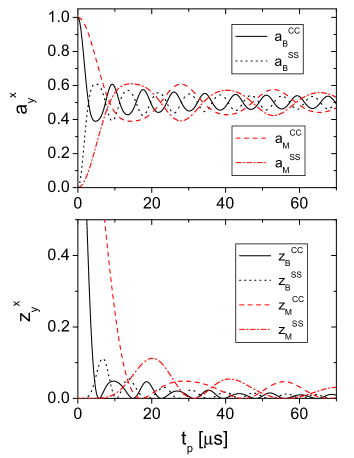
Figure 1: Initial correlations $a_{y}^{x}(t_{p})$ and residual correlations $z_{y}^{x}(t_{p})$ for an isotropic motion, see Eq. (II.2). The values were calculated for anisotropy parameters $\delta_{B}\!=\!2\pi\!\times\!120\mathrm{\,kHz}$ and $\delta_{M}\!=\!2\pi\!\times\!40\mathrm{\,kHz}$.

In Fig. 1, we show theoretical values of the initial and residual correlations $a_{y}^{x}(t_{p})$ and $z_{y}^{x}(t_{p})$, respectively. For the calculation, we used typical anisotropy parameters $\delta_{B}\!=\!2\pi\!\times\!120\mathrm{\,kHz}$ and $\delta_{M}\!=\!2\pi\!\times\!40\mathrm{\,kHz}$.Vogel Due to the periodicity of the sine and cosine functions, all the quantities show an oscillatory behavior with a frequency proportional to the anisotropy parameter. Thus, as a consequence of $\delta_{B}\!\neq\!\delta_{M}$, the ratios $a_{B}^{x}/a_{M}^{x}$ are functions of the evolution time, indicating that the relative contributions of the two deuteron species to the correlation functions depend on the value of $t_{p}$.

SLR and SSR limit the lengths of the interpulse delays in SE experiments. To consider relaxation effects in the second step, we modify Eq. (II.2) according to

$${\cal E}_{2}^{x}(t_{m};t_{p})\!=\!\sum_{y}m_{y}e_{2,y}^{x}(t_{m};t_{p})R_{1,y}(t_{m})R_{2,y}(2t_{p})$$ (11)

While $R_{1,y}(t_{m})$ describes the decrease of the echo height due to SLR during the mixing time, $R_{2,y}(2t_{p})$ quantifies the loss of signal due to SSR during the evolution times, i.e., $R_{i,y}(0)\!=\!1$ and $R_{i,y}(\infty)\!=\!0$ ($i\!=\!1,2$). In analogy with Eq. (4), we define ${\cal F}_{2}^{x}(t_{m};t_{p})\!=\!{\cal E}_{2}^{x}(t_{m};t_{p})/{\cal E}_{2}^{x}(0;t_{p})$. The symbols ${\cal E}_{2}^{x}$ and ${\cal F}_{2}^{x}$ are used to stress that the correlation functions are affected by relaxation effects. As a consequence of fast methyl group rotation at the studied temperatures, the SLR times of the M deuterons are shorter than that of the B deuterons, $T_{1,M}\!\ll\!T_{1,B}$.Vogel Furthermore, the deuteron species exhibit different SSR and, hence, the ratio of the respective contributions to the correlation functions increasingly deviates from the theoretical value $a_{B}^{x}(t_{p})/a_{M}^{x}(t_{p})$, when the evolution time is increased, see Appendix.

The time window of the experiment is limited in particular by the fast SLR of the M deuterons at the studied temperatures, $T_{1,M}\!\approx\!10\mathrm{\,ms}$. Thus, correction for SLR is desirable so as to extend the time window. In ²H NMR, such correction is not possible for the sin-sin correlation functions, since the decay of Alignment order, which is present during the mixing time of this experiment, is not accessible in an independent measurement so that the damping due to SLR is unknown. By contrast, for the cos-cos correlation functions, the decay of Zeeman order, which exists during the mixing time of this measurement, can be determined in a regular SLR experiment. In previous ²H NMR SE studies, it thus proved useful to focus on the cos-cos correlation function and to divide ${\cal E}_{2}^{CC}$ by the SLR function $R_{1}(t_{m})$ to remove SLR effects.

Following an analogous approach, we analyze the correlation functions

$$F_{2}^{*}(t_{m};t_{p})=\frac{{\cal E}_{2}^{CC}(t_{m};t_{p})}{\sum_{y}m_{y}\,a_{y}^{CC}(t_{p})\,R_{1,y}(t_{m})R_{2,y}(2t_{p})}$$ (12)

Here, the denominator can be regarded as an effective SLR function. This function takes into account that the contributions of the B and the M deuterons to the cos-cos correlation function are weighted with the initial correlations $a_{y}^{CC}(t_{p})$. Moreover, it includes that the relative contributions of the two species change due to diverse SSR, as is evident from the factors $R_{2,y}(2t_{p})$.

In the Appendix, we discuss whether this approach enables correction for SLR. Our considerations show that, when two (or more) deuteron species contribute to the cos-cos correlation functions, elimination of relaxation effects is successful only when three conditions are met: (i) Both species exhibit the same dynamical behavior, i.e., $\phi_{B}^{CC}(t_{m};t_{p})\!=\!\phi_{M}^{CC}(t_{m};t_{p})$, which is fulfilled to a good approximation in our case, see Sec. IV.2. (ii) Appropriate evolution times are used so that $z_{B}^{CC}\!=\!z_{M}^{CC}\!\approx\!0$. (iii) The data are corrected utilizing the effective SLR function defined in Eq. (12). The experimental determination of this function is described in the Appendix. In the following, we will mostly focus on evolution times, for which correction for SLR is possible, i.e., $F_{2}^{*}(t_{m};t_{p})\!\approx\!F_{2}^{CC}(t_{m};t_{p})$. In these cases, the corrected data will be referred to as $F_{2}^{CC}$, while we will use $F_{2}^{*}$ to denote situations, when elimination of SLR effects is not successful.

II.3 ⁷Li NMR stimulated-echo spectroscopy

Since the methodologies of ²H and ⁷Li NMR SE spectroscopies are very similar, we restrict ourselves to point out some differences. In ⁷Li NMR, the use of appropriate three-pulse sequences allows one to measure $F_{2}^{SS}$, whereas $F_{2}^{CC}$ is not accessible for $I\!=\!3/2$.BoJMR Moreover, the shape of the quadrupolar coupling tensor is well defined in ²H NMR, while it is subject to a broad distribution in ⁷Li NMR, leading to a damping of the oscillatory behavior of the initial and final correlations, in particular, $z^{SS}\!=\!0$ for sufficiently long evolution times. Furthermore, in our case, ⁷Li SLR is slow so that correction of the ⁷Li NMR correlation functions for relaxation effects is not necessary. Finally, we again emphasize that both ion and polymer dynamics can contribute to the decays of ⁷Li NMR correlation functions and, hence, their interpretation is not as straightforward as for the ²H NMR analogs.

III Experiment

In addition to neat PPO, we study the polymer electrolytes 30:1 PPO-LiClO₄, 15:1 PPO-LiClO₄ and 6:1 PPO-LiClO₄. In the following, we will refer to these samples as PPO, 30:1 PPO, 15:1 PPO and 6:1 PPO. In all samples, we use a deuterated polymer [CD₂-CD(CD₃)-O]_n with a molecular weight $M_{w}\!=\!\mathrm{6510\,g/mol}$. Strictly speaking, the polymer is poly(propylene glycol), having terminal OH groups. The sample preparation was described in our previous work.Vogel In DSC experiments,Vogel we found $T_{g}\!=\!\mathrm{203\pm 2\,K}$ for both PPO and 30:1 PPO and $T_{g}\!=\!\mathrm{272\pm 2\,K}$ for 6:1 PPO. For the intermediate 15:1 composition, we observed a broad glass transition step ranging from about $\mathrm{205\,K}$ to $\mathrm{245\,K}$. In the literature, two glass transition temperatures $T_{g,1}\!\approx\!\mathrm{208\,K}$ and $T_{g,2}\!\approx\!\mathrm{240\,K}$ were reported for 16:1 PPO-LiClO₄.Vachon_1

The ²H NMR experiments were performed on Bruker DSX 400 and DSX 500 spectrometers working at Larmor frequencies $\omega_{0}/2\pi$ of $\mathrm{61.4\,MHz}$ and $\mathrm{76.8\,MHz}$, respectively. Two Bruker probes were used to apply the radio frequency pulses, resulting in $90^{\circ}$ pulse lengths of $\mathrm{2.2\,\mu s}$ and $\mathrm{3.5\,\mu s}$. Comparing results for different setups, we determined that the results depend neither on the magnetic field strength nor on the probe, see Sec. IV.1. The ⁷Li NMR measurements were carried out on the DSX 500 spectrometer working at a Larmor frequency of $\mathrm{194.4\,MHz}$. In these experiments, the $90^{\circ}$ pulse length amounted to $\mathrm{2.5\,\mu s}$. Further experimental details can be found in our previous work.Vogel

Appropriate three-pulse sequences $P_{1}$ - $t_{p}$ - $P_{2}$ - $t_{m}$ - $P_{3}$ - $t$ are sufficient to measure sin-sin and cos-cos correlation functions for sufficiently large evolution times. However, for short evolution times, the stimulated echo, which occurs at $t\!=\!t_{p}$, vanishes in the dead time of the receiver, following the excitation pulses.Spiess ; Roessler This problem can be overcome, when a fourth pulse is added to refocus the stimulated echo outside the dead time, leading to four-pulse sequences $P_{1}$ - $t_{p}$ - $P_{2}$ - $t_{m}$ - $P_{3}$ - $\Delta$ - $P_{4}$.Spiess ; Roessler We use three-pulse and four-pulse sequences to measure correlation functions for large ($t_{p}\!=\!60\mathrm{\,\mu s}$) and small ($t_{p}\!=\!2\mathrm{\,\mu s}$) evolution times, respectively. When we study the dependence of the cos-cos correlation functions on the evolution time, we apply a four-pulse sequence for all values of $t_{p}$. In all experiments, we use suitable phase cycles to eliminate unwanted signal contributions.Schaefer_PC

IV Results

IV.1 Temperature dependent ²H NMR correlation functions

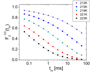
Figure 2: Correlation functions $F_{2}^{CC}(t_{m};t_{p}\!=\!60\mathrm{\,\mu s})$ for neat PPO at various temperatures. The dashed lines are fits to Eq. (13) with $\beta\!=\!0.33$ and $C\!=\!0.01$.

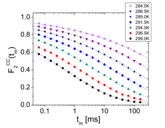
Figure 3: Correlation functions $F_{2}^{CC}(t_{m};t_{p}\!=\!60\mathrm{\,\mu s})$ for 6:1 PPO-LiClO₄ at various temperatures. The dashed lines are fits to Eq. (13) with $\beta\!=\!0.24$ and $C\!=\!0.01$.

In Figs. 2 and 3, we show temperature dependent correlation functions $F_{2}^{CC}(t_{m};t_{p}\!=\!60\mathrm{\,\mu s})$ for PPO and 6:1 PPO. Due to the finite pulse lengths this value of $t_{p}$ corresponds to an effective evolution time of about $62\mathrm{\,\mu s}$, see Sec. IV.2, so that the residual correlation for both deuteron species approximately vanishes and, hence, correction for SLR is possible. Furthermore, we will show in Sec. IV.2 that, for this large evolution time, $F_{2}^{CC}(t_{m};t_{p})$ approximates the jump correlation function $F_{2}^{J}(t_{m})$, see Eq. (6). In Figs. 2 and 3, it is evident that both materials exhibit nonexponential correlation functions. Moreover, for the 6:1 polymer electrolyte, the loss of correlation occurs at much higher temperatures in the time window of the experiment, indicating that the presence of salt slows down the polymer segmental motion.

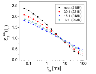
Figure 4: Scaled cos-cos correlation functions for PPO, 30:1 PPO-LiClO₄, 15:1 PPO-LiClO₄ and 6:1 PPO-LiClO₄ ($t_{p}\!=\!60\mathrm{\,\mu s}$). The temperatures are indicated. They are chosen so as to compare correlation functions with similar time constants $\tau\!=\!3.8\!-5.8\mathrm{\,ms}$. For the sake of comparison, the data was scaled according to $S_{2}^{CC}(t_{m})\!=\!F_{2}^{CC}(t_{m})/F_{2}^{CC}(t_{0})$ where $t_{0}\!=\!5.6\mathrm{\,ms}\!\approx\!\tau$. The dashed lines are interpolations with a function proportional to Eq. (13). The used stretching parameters are $\beta\!=\!0.33$ for PPO, $\beta\!=\!0.3$ for 30:1 PPO-LiClO₄, $\beta\!=\!0.2$ for 15:1 PPO-LiClO₄ and $\beta\!=\!0.24$ for 6:1 PPO-LiClO₄.

To study how the presence of salt affects the nonexponentiality of the polymer dynamics, we compare correlation functions $F_{2}^{CC}(t_{m};t_{p}\!=\!60\mathrm{\,\mu s})$ for all studied materials in Fig. 4. The respective temperatures were chosen so as to consider correlation functions with comparable time constants. For the sake of comparison, we actually show scaled correlation functions $S_{2}^{CC}(t_{m})$. We see that the nonexponentiality of the polymer dynamics is not a linear function of the salt content, but it is most pronounced for 15:1 PPO. Assuming that the rate of the segmental motion reflects the local salt concentration, these findings suggest that structural heterogeneities relating to the spatial salt distribution are most pronounced for the intermediate 15:1 composition, while the structure is more homogeneous for higher and lower salt contents.

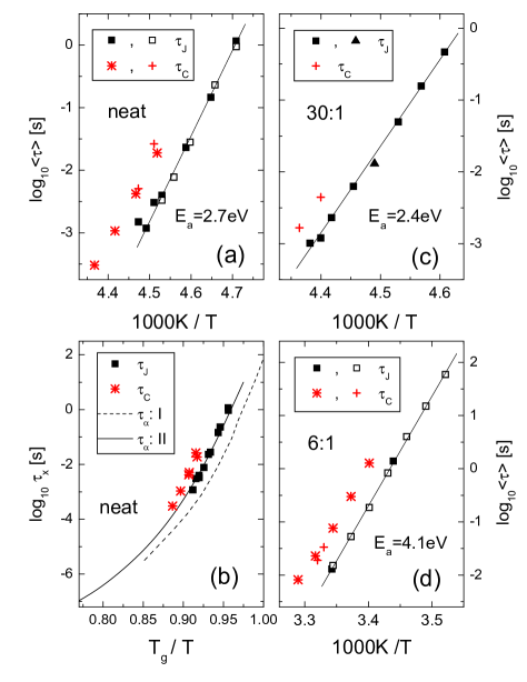
Figure 5: Mean correlation times for (a) PPO, (c) 30:1 PPO-LiClO₄ and (d) 6:1 PPO-LiClO₄. The time constants $\langle\tau_{C}\!\rangle$ and $\langle\tau_{J}\!\rangle$ result from interpolations of $F_{2}^{SS}(t_{m};t_{p}\!=\!2\mathrm{\,\mu s})$ and $F_{2}^{CC}(t_{m};t_{p}\!=\!60\mathrm{\,\mu s})$ with Eq. (13), respectively. While the time constants shown as open squares and crosses were obtained for $\omega_{0}/(2\pi)\!=\!61.4\mathrm{\,MHz}$, that displayed as solid squares and stars were determined for $\omega_{0}/(2\pi)\!=\!76.8\mathrm{\,MHz}$. For 30:1 PPO-LiClO₄, the solid triangle is a data point resulting from experiments using a four-pulse rather than a three-pulse sequence. In panel (b), we compare our results for PPO with correlation times $\tau_{\alpha}$ from dielectric spectroscopy (I: Ref. Leon, , II: Ref. Furukawa, ). The correlation times are shown on a reduced $T_{g}/T$ scale to remove effects due to different glass transition temperatures, $T_{g}\!=\!203\mathrm{\,K}$ and $T_{g}\!=\!198\mathrm{\,K}$.Furukawa ; Leon The latter difference reflects the fact that polymers with a smaller molecular weight $M_{w}\!=\!\mathrm{4000\,g/mol}$ were investigated in the previous approaches.Furukawa ; Leon

For a quantitative analysis of the correlation functions $F_{2}^{CC}(t_{m};t_{p}\!=\!60\mathrm{\,\mu s})$, we fit the data for all compositions and temperatures with a modified KWW function

$$(1-C)\exp\left[-\left(\frac{t}{\tau}\right)^{\beta}\right]+C$$ (13)

At high temperatures, when the decay to the final state value can be observed in our time window, we obtain small residual correlations $C\!=\!0.01\!\pm\!0.01$, in harmony with the theoretical value for this evolution time, see Fig. 1. Therefore, we keep this value fixed in the fits for the lower temperatures. For neither of the materials, we find evidence for a systematic temperature dependence of the stretching parameter $\beta$. Specifically, we observe values $\beta\!=\!0.33\!\pm\!0.02$ for PPO, $\beta\!=\!0.30\!\pm\!0.02$ for 30:1 PPO and $\beta\!=\!0.24\!\pm\!0.02$ for 6:1 PPO. For the 15:1 composition, determination of the stretching parameter is somewhat ambiguous due to the extreme nonexponentiality. However, for all studied temperatures, a reasonable interpolation of the data can be obtained with $\beta\!=\!0.2$, as will be discussed in more detail in Sec. IV.3. Hence, the values of the stretching parameters confirm that the nonexponentiality of the segmental motion depends on the salt concentration.

The mean correlation times can be obtained according to $\langle\tau\rangle\!=\!(\tau/\beta)\,\Gamma(1/\beta)$ from the fit parameters, where $\Gamma(x)$ is the $\Gamma$ function. In the following, we denote the mean time constants resulting for $t_{p}\!=\!60\mathrm{\mu s}$ as mean jump correlation times $\langle\tau_{J}\rangle$, since correlation functions for this relatively large evolution time approximate $F_{2}^{J}(t_{m})$, see Sec. IV.2. The mean jump correlation times for PPO, 30:1 PPO and 6:1 PPO are shown in Fig. 5. We see that, for $T_{g}\!<\!T\!\lesssim\!1.1\,T_{g}$, the temperature dependence of $\langle\tau_{J}\rangle$ is well described by an Arrhenius law. While we find similar activation energies $E_{a}\!=\!2.7\!\pm\!0.2\mathrm{\,eV}$ and $E_{a}\!=\!2.4\!\pm\!0.2\mathrm{\,eV}$ for PPO and 30:1 PPO, respectively, there is a higher value $E_{a}\!=\!4.1\!\pm\!0.2\mathrm{\,eV}$ for 6:1 PPO. The higher activation energy for the latter composition is consistent with the slowing down of the segmental motion for high salt concentrations. In addition, we see in Fig. 5 that the correlation times are independent of the experimental setup, as one would expect.

To obtain an estimate of the ”NMR glass transition temperature”, we extrapolate the Arrhenius temperature dependence of the mean jump correlation time and determine the temperatures at which $\langle\tau_{J}\rangle\!=\!100\mathrm{\,s}$. We find temperatures $205\mathrm{\,K}$ for PPO ($T_{g}\!=\!203\mathrm{\,K}$), $208\mathrm{\,K}$ for 30:1 PPO ($T_{g}\!=\!203\mathrm{\,K}$) and $283\mathrm{\,K}$ for 6:1 PPO ($T_{g}\!=\!272\mathrm{\,K}$), which are in reasonable agreement with the calorimetrically determined values of $T_{g}$. Thus, the slowing down of the segmental motion upon addition of salt reflects the shift of the glass transition temperature.

Next, we focus on $F_{2}^{SS}(t_{m};t_{p}\!=\!2\mathrm{\,\mu s})\!\approx\!F_{2}(t_{m})$. Since correction for SLR is not possible for sin-sin correlation functions, see Sec. II.2, this analysis is restricted to relatively high temperatures at which segmental motion is faster than SLR. In Fig. 5, we include the mean correlation times $\langle\tau_{C}\rangle$, as obtained from fits of $F_{2}^{SS}(t_{m};t_{p}\!=\!2\mathrm{\,\mu s})$ to Eq. (13). We see that $\langle\tau_{C}\rangle$ and $\langle\tau_{J}\rangle$ exhibit a comparable temperature dependence. For all compositions, $\langle\tau_{C}\rangle$ is about one order of magnitude longer than $\langle\tau_{J}\rangle$. Thus, a similar ratio $\langle\tau_{J}\rangle/\langle\tau_{C}\rangle\!\approx\!0.1$ implies that the presence of salt does not affect the jump angles of the segmental motion. Using this ratio in Eq. (7), we obtain a mean jump angle $\gamma\!=\!15^{\circ}$. Hence, the segmental motion involves rotational jumps about small angles both in the absence and in the presence of salt. In Sec. IV.2, the dependence of the mean correlation time on the evolution time, $\langle\tau(t_{p})\rangle$, will be studied in more detail.

In dielectric spectroscopy, it was found that a Vogel-Fulcher behavior describes the temperature dependence of the $\alpha$ process of PPO in the presence and in the absence of salt.Furukawa ; Leon ; Johari Thus, on first glance, it is surprising that the correlation times follow an Arrhenius law in our case. For PPO, we show $\langle\tau_{J}(T)\rangle$ and $\langle\tau_{C}(T)\rangle$ together with dielectric data $\tau_{\alpha}(T)$Furukawa ; Leon in Fig. 5(b). The time constants are plotted on a reduced $T_{g}/T$ scale to remove effects resulting from the somewhat different glass transition temperatures of the studied polymers. Considering the error resulting from this scaling, we conclude that our results are in reasonable agreement with the literature data. In particular, all the curves exhibit, if at all, a very small curvature in the temperature range $0.9\!<\!T_{g}/T\!<\!1$, rationalizing that an Arrhenius law enables a good description of the temperature dependence in this regime. At higher temperatures, the dielectric data show a pronounced curvature in the Arrhenius representation, as described by the Vogel-Fulcher behavior. In our case, the observation of unphysical pre-exponential factors $\tau_{0}\!=\!10^{-56}\!-\!10^{-71}\mathrm{\,s}$ implies a breakdown of the Arrhenius law at higher temperatures. Consistently, a previous SE study on the $\alpha$ process of a polymer melt reported prefactors $\tau_{0}\!\approx\!10^{-77}\mathrm{\,s}$ from Arrhenius interpolations of temperature dependent correlation times.Tracht Hence, SE spectroscopy yields apparent activation energies $E_{a}$, characterizing the strong temperature dependence of the segmental motion close to $T_{g}$, while deviations from an Arrhenius law become evident when following $\tau_{\alpha}(T)$ to higher temperatures.

IV.2 ²H NMR correlation functions for various relaxation delays and evolution times

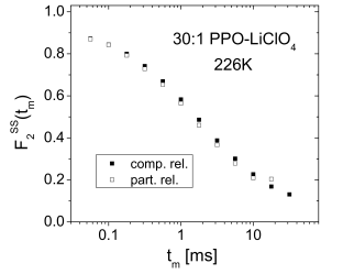
Figure 6: Correlation functions $F_{2}^{SS}(t_{m};t_{p}\!=\!2\mathrm{\,\mu s})$ for 30:1 PPO-LiClO₄ at $T\!=\!226\mathrm{\,K}$. The measurements were performed for complete recovery ($t_{R}\!=\!1\mathrm{\,s}\!\gg\!T_{1,B}$) and partial recovery ($t_{R}\!=\!3\mathrm{\,ms}\!\ll\!T_{1,B}$) of the magnetization after saturation.

Next, we study whether different structural units of the PPO molecule show distinguishable reorientation behavior. Exploiting that $T_{1,M}\!\ll\!T_{1,B}$ for PPO and 30:1 PPO at $T\!\approx\!T_{g}$,Vogel we record correlation functions for different relaxation delays $t_{R}$ between the saturation of the magnetization and the start of the SE pulse sequence. Then, the contribution of the M deuterons can be singled out in partially relaxed experiments, i.e., for $t_{R}\!\approx\!T_{1,M}\!\ll\!T_{1,B}$, while, of course, both deuteron species will contribute to the correlation functions if we wait until the recovery of the magnetization is complete.

In Fig. 6, we display completely relaxed and partially relaxed correlation functions for 30:1 PPO at $T\!=\!226\mathrm{\,K}$. Evidently, $F_{2}^{SS}(t_{m};t_{p}\!=\!2\mathrm{\,\mu s})$ is independent of the relaxation delay $t_{R}$, indicating that the ”relevant” rotational jumps of the B and the M deuterons occur on essentially the same time scale. Here, the term ”relevant” is used to denote the situation that the threefold jumps of the methyl group are not probed in the present approach. Performing an analogous analysis for neat PPO, we arrive at the same conclusion. Partially and completely relaxed correlation functions for larger values of $t_{p}$ will be compared below.

Figure 7: Residual correlations from interpolations of cos-cos correlation functions for PPO at $T\!=\!222\mathrm{\,K}$ with Eq. (13). The top and bottom panel show data obtained for partial and complete recovery of the magnetization, respectively. The lines are theoretical values $z_{y}^{CC}/a_{y}^{CC}$ for $\delta_{M}\!=\!2\!\pi\times\!39\mathrm{\,kHz}$ (top panel) and $\delta_{B}\!=\!2\!\pi\times\!119\mathrm{\,kHz}$ (bottom panel)

In previous work on molecular and polymeric glass formers, it was demonstrated that more detailed insights into the reorientational mechanisms are possible when $F_{2}^{CC}(t_{m};t_{p})$ is recorded for many evolution times.Roessler ; Geil ; Hinze ; BoHi ; Tracht For example, information about the shape of the distribution of jump angles is available from the dependence of the mean correlation time on the evolution time, $\langle\tau(t_{p})\rangle$. Hence, it is desirable to apply this approach also to polymer electrolytes PPO-LiClO₄. However, in our case, the presence of two deuteron species hampers straightforward analysis of $F_{2}^{CC}(t_{m};t_{p})$ for an arbitrary value of $t_{p}$, see Sec. II.2. In the following, we test three approaches aiming to extract $\langle\tau(t_{p})\rangle$ in such situation.

In approach (A), we measure partially relaxed correlation functions $F_{2}^{CC}(t_{m};t_{p})$. Then, the signal solely results from the M deuterons and correction for SLR is possible for all values of $t_{p}$ when the data is divided by the relaxation function $R_{1,M}(t_{m})$, which can be obtained from SLR measurements. Thus, it is possible to determine $\langle\tau(t_{p})\rangle$ from fits of the corrected data to Eq. (13). To demonstrate that this approach indeed allows us to single out the contribution of the M deuterons, we show experimental and theoretical values of the residual correlation $F_{2}^{CC}(\infty;t_{p})$ as a function of $t_{p}$ in Fig. 7. The experimental values result from interpolations of the partially relaxed correlation functions $F_{2}^{CC}(t_{m};t_{p})$ for PPO at $T\!=\!222\mathrm{\,K}$. The theoretical values were obtained by calculating $z_{M}^{CC}(t_{p})/a_{M}^{CC}(t_{p})$ for $\delta_{M}\!=\!2\pi\times 39\mathrm{\,kHz}$.Vogel Obviously, the experimental and the theoretical curves $F_{2}^{CC}(\infty;t_{p})$ nicely agree, when we shift the measured data by $1.5\mathrm{\,\mu s}$ to longer evolution times. This shift reflects the fact that, due to finite pulse lengths, the effective evolution times are $1\!-\!2\mathrm{\,\mu s}$ longer than the set values, as was reported in previous work.BoHi The good agreement of experimental and theoretical residual correlations indicates that approach (A) allows us to study the reorientational mechanisms of the methyl group axes. However, this approach is restricted to PPO and 30:1 PPO since $T_{1,M}$ and $T_{1,B}$ differ less for higher salt concentrations,Vogel hampering a suppression of contributions from the B deuterons in partially relaxed experiments.

In approaches (B) and (C), we focus on completely relaxed correlation functions. Then, we can include 6:1 PPO, for which the salt should have the strongest effect on the segmental motion. In both approaches, the measured decays for different evolution times are divided by the corresponding effective SLR functions, which are determined in concomitant SLR measurements, as is described in the Appendix. To emphasize that correction for SLR is not successful when $z_{B}^{CC}(t_{p}),z_{M}^{CC}(t_{p})\!\neq\!0$, we denote the resulting data as $F_{2}^{*}(t_{m};t_{p})$, see Eq. (12).

In approach (B), we extract $\langle\tau(t_{p})\rangle$ from interpolations of $F_{2}^{*}(t_{m};t_{p})$ with Eq. (13). In doing so, we disregard that the residual correlation depends on the mixing time at $t_{m}\!\approx\!T_{1,M}$, see Appendix. In the limit $t_{m}\!\rightarrow\!\infty$, a residual correlation $F_{2}^{*}(\infty;t_{p})\!=\!z_{B}^{CC}(t_{p})/a_{B}^{CC}(t_{p})$ is expected based on Eq. (14). Figure 7 shows the residual correlation obtained from completely relaxed correlation functions $F_{2}^{*}(t_{m};t_{p})$ for PPO at $T\!=\!222\mathrm{\,K}$ together with the theoretical curve $z_{B}^{CC}(t_{p})/a_{B}^{CC}(t_{p})$ for $\delta_{B}\!=\!2\pi\times 119\mathrm{\,kHz}$.Vogel Shifting the measured points again by $1.5\mathrm{\,\mu s}$, a good agreement of the experimental and the theoretical data is obtained, confirming our expectations for the residual correlation. Therefore, we use the theoretical values of $F_{2}^{*}(\infty;t_{p})$ in a second round of fitting to reduce the number of free parameters and the scattering of the data.

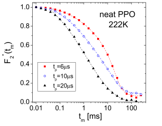
Figure 8: $F_{2}^{*}(t_{m};t_{p})$ for PPO at $T\!=\!222\mathrm{\,K}$. The evolution times $t_{p}$ are indicated. The dashed lines are fits with Eq. (12). See text for details.

In approach (C), we employ Eq. (12) to fit $F_{2}^{*}(t_{m};t_{p})$. In doing so, we use the theoretical values of $z_{y}^{CC}(t_{p})$ and $a_{y}^{CC}(t_{p})$ together with the relaxation functions $R_{1,y}$ and $R_{2,y}$ from independent SLR measurements, see Appendix. Considering our result that the relevant rotational jumps of the B and the M deuterons occur on very similar time scales, see Fig. 6, we utilize the same correlation function $\phi(t_{m};t_{p})$ for both deuteron species. Assuming a KWW function, we have two free fit parameters, $\tau$ and $\beta$. In Fig. 8, we show examples of $F_{2}^{*}(t_{m};t_{p})$ for PPO at $T\!=\!222\mathrm{\,K}$. Evidently, approach (C) enables a good description of the data for all values of $t_{p}$.

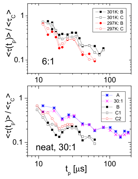
Figure 9: Scaled mean correlation times $\langle\tau(t_{p})\rangle/\langle\tau_{C}\rangle$ for PPO at $T\!=\!222\mathrm{\,K}$ and 6:1 PPO-LiClO₄ at $T\!=\!297\mathrm{\,K}$ and $T\!=\!301\mathrm{\,K}$. Results from approach (B) and approach (C) are included. For PPO, we compare data from two independent measurements (C1,C2). In addition, we show the scaled mean correlation times from partially relaxed experiments for PPO at $T\!=\!222\mathrm{\,K}$ and for 30:1 PPO-LiClO₄ at $T\!=\!226\mathrm{\,K}$ ($t_{R}\!=\!3\mathrm{\,ms}$), which were obtained using approach (A). See text for details.

In Fig. 9, we present mean correlation times $\langle\tau(t_{p})\rangle$ resulting from the described approaches for PPO, 30:1 PPO and 6:1 PPO. Strictly speaking, the scaled data $\widetilde{\tau}(t_{p})\!\equiv\!\langle\tau(t_{p})\rangle/\langle\tau_{C}\rangle$ are shown for the sake of comparison. Inspecting the results of the partially relaxed experiments, it is evident that the rotational jumps in PPO and 30:1 PPO are characterized by very similar curves $\widetilde{\tau}(t_{p})$. Hence, the threefold methyl group axes show essentially the same reorientational mechanism in both materials. In particular, for both compositions, the dependence on the evolution time is weak for $t_{p}\!>\!60\mathrm{\,\mu s}$, indicating that the jump correlation function $F_{2}^{J}(t_{m})$ is approximately measured. Thus, $\widetilde{\tau}(t_{p}\!>\!60\mathrm{\,\mu s})$ provides an estimate for $\langle\tau_{J}\rangle/\langle\tau_{C}\rangle$. Using a typical value $\widetilde{\tau}\!=\!0.15$, Eq. (7) yields a mean jump angle $\gamma\!=\!18^{\circ}$ for the rotational jumps of the methyl-group axes.

Next, we focus on the outcome of the completely relaxed experiments in Fig. 9. Although approaches (B) and (C) give somewhat different results, the overall shape of the respective curves $\widetilde{\tau}(t_{p})$ is still comparable. In particular, the findings for sufficiently large evolution times are in good agreement due to small values of the residual correlations $z_{y}^{x}(t_{p})$, see Fig. 1. We conclude that semiquantitative information about the reorientational mechanism is available in our case of two deuteron species. While the data allows us to compare the results for different salt concentrations and to extract mean jump angles, we refrain from determination of the distribution of jump angles from further analysis of $\widetilde{\tau}(t_{p})$, since the error is too big to resolve details of the shape of this distribution. We estimate the data to be correct within a factor of two. The rough agreement of the curves $\widetilde{\tau}(t_{p})$ for PPO and 6:1 PPO nevertheless indicates that the presence of salt, if at all, has a weak effect on the reorientational mechanism of the polymer segments, in harmony with the results in Fig. 5. In Fig. 9, we further see that $\widetilde{\tau}(t_{p})$ weakly depends on $t_{p}$ for $t_{p}\!>\!40\mathrm{\,\mu s}$, justifying our argument $F_{2}^{CC}(t_{m};t_{p}\!=\!60\mathrm{\,\mu s})\!\approx\!F_{2}^{J}(t_{m})$. For both materials, we find $\widetilde{\tau}(t_{p}\!>\!40\mathrm{\,\mu s})\!=\!0.1\!-\!0.2$, corresponding to mean jump angles $\gamma\!=\!15\!-\!21^{\circ}$.

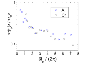
Figure 10: Scaled mean correlation times $\langle\tau(t_{p})\rangle/\langle\tau_{C}\rangle$ from partially relaxed (A) and completely relaxed (C1) correlation functions for PPO at $T\!=\!222\mathrm{\,K}$. The data is the same as in Fig. 9, but it is now shown on a reduced $\delta t_{p}$ scale. We used $\delta_{M}\!=\!2\!\pi\times\!39\mathrm{\,kHz}$ and $\delta_{B}\!=\!2\!\pi\times\!119\mathrm{\,kHz}$ for the partially and the completely relaxed data, respectively.

In Fig. 10, we replot the results from the partially and the completely relaxed experiments for PPO at $T\!=\!222\mathrm{\,K}$ on a reduced $\delta t_{p}$ scale. In this way, we can alleviate effects due to the difference of the anisotropy parameters $\delta_{M}\!\neq\!\delta_{B}$. The good agreement of the completely and the partially relaxed data indicates that the relevant rotational jumps of the B and the M deuterons are similar not only with respect to the time scale, see Fig. 6, but also with respect to the reorientational mechanism. Some deviations are expected since M and B deuterons contribute to the completely relaxed data and, hence, complete elimination of effects due to the different anisotropy parameters is not possible.

IV.3 ²H NMR and ⁷Li NMR correlation functions for 15:1 PPO-LiClO₄

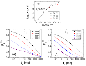
Figure 11: Correlation functions for 15:1 PPO-LiClO₄ at the indicated temperatures: (a) $F_{2}^{SS}(t_{m};t_{p}\!=\!60\mathrm{\,\mu s})$ from ⁷Li NMR and (b) $F_{2}^{CC}(t_{m};t_{p}\!=\!60\mathrm{\,\mu s})$ from ²H NMR. The dashed lines are fits with a KWW function, see Eq. (13), where $C\!=\!0.00$ and $C\!=\!0.01$ for ⁷Li and ²H NMR, respectively. The dotted lines are interpolations of the ⁷Li NMR data for $T\!=\!253\mathrm{\,K}$ and $T\!=\!263\mathrm{\,K}$ with a two-step decay. (c) Mean correlation times $\langle\tau_{J}\rangle$ determined based on the KWW fits of the ²H and ⁷Li NMR results. We also include time constants obtained from measurements of $F_{2}^{SS}(t_{m};t_{p}\!=\!60\mathrm{\,\mu s})$ in ²H NMR.

In Fig. 11, we compare ²H and ⁷Li NMR correlation functions for 15:1 PPO. It is evident that the correlation functions for both nuclei decay on similar time scales, suggesting a coupling of ion and polymer dynamics. In ²H NMR, reasonable interpolations of $F_{2}^{CC}(t_{m};t_{p}\!=\!60\mathrm{\,\mu s})$ are obtained for all studied temperatures when we use a KWW function with $\beta\!=\!0.2$. However, closer inspection of the data reveals some deviations from a KWW behavior. Considering that a coexistence of fast and slow polymer dynamics was reported for compositions of about 15:1 PPO-LiClO₄,Furukawa ; Bergman one may speculate that a fit with two Kohlrausch functions gives a better description of the ²H NMR correlation functions. However, the limited time window does not allow us an unambiguous decision. In any case, the shape of the ²H NMR correlation function shows that if fast and slow polymer dynamics exist the corresponding rate distributions will overlap in large parts so that there is no true bimodality. The ⁷Li NMR correlation functions $F_{2}^{SS}(t_{m};t_{p}\!=\!60\mathrm{\,\mu s})$ for $T\!<\!250\mathrm{\,K}$ are well described by a KWW function with $\beta\!\approx\!0.24$. At higher temperatures, two-step decays are evident, suggesting the presence of two distinguishable lithium species. However, since the interpretation of ⁷Li NMR data for polymer electrolytes has not yet been established, this tentative speculation deserves a careful check in future work, see Sec. II.1.

The mean time constants resulting from the KWW fits of the ²H and ⁷Li NMR correlation functions are compiled in Fig. 11(c). At variance with the results for the other compositions, the mean jump correlation times $\langle\tau_{J}\rangle$ extracted from the ²H NMR data for 15:1 PPO do not follow an Arrhenius law. For $T\!>\!245\mathrm{\,K}$, the temperature dependence is described by $E_{a}\!=\!2.4\mathrm{\,eV}$, which is consistent with the apparent activation energies for PPO and 30:1 PPO, see Fig. 5. However, the variation of $\langle\tau_{J}\rangle$ with temperature is weaker at lower temperatures. There are two possible explanations for the latter behavior. On the one hand, it is possible that a description using a single KWW function is not appropriate due to an existence of fast and slow polymer dynamics. On the other hand, it was demonstrated that the decay times of correlation functions do no longer reflect the shift of a distribution of correlation times when this distribution is much broader than the experimental time window,Vogel_1 ; Vogel_2 as one may expect for 15:1 PPO.Vogel Rather, due to interference with the experimental time window, the decay times feign a weaker temperature dependence,Vogel_3 as is observed in our case. The mean correlation times resulting from the ⁷Li NMR experiments are comparable to the corresponding ²H NMR data. This finding suggests a coupling of ion and polymer dynamics, as was inferred from visual inspection of the correlation functions. However, we again emphasize that, in studies on the ion dynamics in polymer electrolytes, the interpretation of ⁷Li NMR experiments is not yet clear.

V Summary and Conclusion

We demonstrated that ²H NMR SE spectroscopy provides straightforward access to both the time scale and the geometry of slow polymer segmental motion in polymer electrolytes. Here, we exploited these capabilities for an investigation of PPO, 30:1 PPO-LiClO₄, 15:1 PPO-LiClO₄ and 6:1 PPO-LiClO₄. Comparison of the results for the different salt concentrations gives clear evidence that addition of salt leads to a strong slowing down of the polymer dynamics, while the geometry of the segmental motion is hardly affected.

The dependence of the ²H NMR correlation functions on the evolution time yields quantitative information about the geometry of the segmental reorientation.Fujara_1 ; Roessler This possibility results from the fact that the evolution time has the meaning of a geometrical filter. The jump angles of rotational jumps can be determined from the variation of the mean correlation time with the evolution time, $\langle\tau(t_{p})\rangle$.Geil ; Hinze ; BoHi ; Tracht For PPO and 6:1 PPO, we found comparable curves $\langle\tau(t_{p})\rangle$, indicating that the polymer segments exhibit similar jump angle distributions in the presence and in the absence of salt. Furthermore, we exploited that the mean jump angle can be determined from the ratio of the jump correlation time $\langle\tau_{J}\rangle$ and the overall correlation time $\langle\tau_{C}\rangle$, which can be extracted from the ²H NMR correlation functions in the limits $t_{p}\!\rightarrow\!\infty$ and $t_{p}\!\rightarrow\!0$, respectively. For PPO, 30:1 PPO and 6:1 PPO, a ratio of about 0.1 corresponds to a mean jump angle of ca. 15^∘. In the case of PPO, this value is consistent with results for various neat polymers,Spiess ; Wefing ; Kaufmann ; Pschorn ; Schaefer ; Tracht suggesting that small angle rotational jumps are typical of polymer segmental motion close to $T_{g}$. For the polymer electrolytes, the agreement of the mean jump angles confirms that the reorientational mechanism is essentially independent of the salt concentration.

In general, trans-gauche conformational transitions are attributed to the $\alpha$ process, implying the existence of large angle jumps. Thus, it may be surprising that the present and previous NMR studies on polymer melts and polymer electrolytes find small jump angles of $10\!-\!40^{\circ}$. To rationalize the latter behavior, the cooperativity of the $\alpha$ process was taken into account in the literature.Tracht Specifically, it was argued that concerted conformational transitions of neighboring polymer segments lead to jump angles that are not well-defined and smaller than the angles typical of conformational transitions.

Comparing the correlation times for the different mixtures PPO-LiClO₄, we quantified the slowing down of the segmental motion as a consequence of the presence of salt. For PPO, the mean jump correlation time amounts to $\langle\tau_{J}\rangle\!=\!1\mathrm{\,s}$ at $T\!=\!212\mathrm{\,K}$, whereas, for the highest salt concentration, 6:1 PPO, it has this value at $T\!=\!292\mathrm{\,K}$. Considering the strong temperature dependence of polymer dynamics close to $T_{g}$, the difference $\Delta T\!=\!\mathrm{80\,K}$ shows that addition of salt results in an enormous slowing down of the polymer segmental motion. This finding is consistent with both pronounced effects on the glass transition temperature and results from previous work.Carlsson_2 ; Johari

In the studied temperature ranges of $T_{g}\!<\!T\!\lesssim\!1.1\,T_{g}$, the temperature dependence of the mean jump correlation time $\langle\tau_{J}\rangle$ follows an Arrhenius law. While we observed apparent activation energies $E_{a}\!\approx\!2.5\mathrm{\,eV}$ for the neat polymer and the moderate salt concentrations, a higher value $E_{a}\!\approx\!4.1\mathrm{\,eV}$ characterizes the segmental motion in 6:1 PPO. Likewise, the mean correlation time $\langle\tau_{C}\rangle$, characterizing the rotational correlation function of the second Legendre polynomial, shows a substantially stronger temperature dependence for 6:1 PPO than for PPO. Hence, the slowing down of the polymer dynamics for high salt concentrations is also reflected in higher apparent activation energies close to $T_{g}$. For all compositions, the pre-exponential factors of the Arrhenius laws have unphysical values, $\tau_{0}\!=\!10^{-56}\!-\!10^{-71}\mathrm{\,s}$, indicating that there is no simple thermally activated process over a single barrier. Consistently, a Vogel-Fulcher behavior can be used to describe the temperature dependence of the $\alpha$ process in a broader temperature range.Furukawa ; Johari ; Bergman ; Leon

The ²H NMR correlation functions for mixtures PPO-LiClO₄ decay in a strongly nonexponential manner, where the stretching depends on the salt concentration. For the correlation function $F_{2}^{CC}(t_{m};t_{p}\!=\!60\mathrm{\,\mu s})$, we obtained stretching parameters $\beta\!\approx\!0.33$ for PPO, $\beta\!\approx\!0.3$ for 30:1 PPO, $\beta\!\approx\!0.2$ for 15:1 PPO and $\beta\!\approx\!0.24$ for 6:1 PPO, which show no systematic variation with temperature in the range $T_{g}\!<\!T\!\lesssim\!1.1\,T_{g}$. Thus, the nonexponentiality of the segmental motion is most prominent for intermediate salt concentrations of about 15:1, while it is reduced for both low and high salt content. Likewise, previous work reported that polymer dynamics is more nonexponential in the presence than in the absence of salt.Carlsson_2 ; Torell We conclude that the additional structural heterogeneities imposed by the addition of salt have a strong effect on the structural relaxation of the polymer melt.

Comparison of ²H NMR correlation functions for partial and complete recovery of the longitudinal magnetization provided insights into the reorientation of different structural units. With the exception of methyl group rotation, we found no evidence for diverse dynamical behaviors of different structural units. Strictly speaking, the C-D bonds of the ethylene groups and the threefold methyl group axes show comparable rotational jumps with respect to both time scale and jump angles.

All these results of the present ²H NMR SE study are consistent with findings of our previous ²H NMR line-shape analysis for polymer electrolytes PPO-LiClO₄.Vogel Specifically, the ²H NMR spectra gave evidence that the presence of salt slows down the segmental motion. In addition, the ²H NMR spectra indicated that, in large parts, the pronounced nonexponentiality of the polymer dynamics results from the existence of a broad distribution of correlation times $G(\log\tau)$. Then, the stretching parameters $\beta$ are a measure of the decadic width $\Delta$ of this distribution. In detail, the width is given by $\Delta\!\approx\!1.14(0.93/\beta\!+\!0.06)$.BoBe Based on this expression, we obtain widths of $\Delta\!=\!3.3$ and $\Delta\!=\!5.4$ orders of magnitude from the stretching parameters for PPO and 15:1 PPO, respectively. The latter result is in nice agreement with findings from our ²H NMR line-shape analysis for the 15:1 composition.Vogel There, the spectra were described using a logarithmic Gaussian distribution $G(\log\tau)$ with a full width at half maximum of 5-6 orders of magnitude. We conclude that both ²H NMR techniques yield a coherent picture of the segmental motion in polymer electrolytes. However, they highlight different aspects of the dynamics and, hence, a combined approach is particularly useful. While ²H NMR SE spectroscopy is a powerful tool to quantify the time scale and the geometry of the segmental motion, ²H NMR spectra allow one to demonstrate the existence of dynamical heterogeneities provided the distribution $G(\log\tau)$ is sufficiently broad.

Having established that presence of salt slows down the segmental motion, one expects that the shape of the distribution of correlation times governing the polymer dynamics reflects features of the salt distribution in polymer electrolytes PPO-LiClO₄. We observed that the distribution $G(\log\tau)$ is broadest for the 15:1 composition, implying a strong variation in the local salt concentration for this intermediate composition, whereas the spatial distribution of the salt is more homogeneous for both high and low salt content. In the literature, it was proposed that there is liquid-liquid phase separation into salt-rich and salt-depleted regions for intermediate salt concentrations.Vachon_1 ; Vachon_2 ; Furukawa ; Bergman Provided the rate of the segmental motion is a measure of the local salt concentration, the existence of well-defined microphases should lead to a bimodal distribution of correlation times for the polymer dynamics and, consequently, to a two-step decay of the ²H NMR correlation functions. Although there are some indications for the presence of a two-step decay, a KWW function still provides a satisfactory interpolation of the experimental data for 15:1 PPO-LiClO₄. Hence, our results are at variance with a bimodal, discontinuous distribution of correlation times and, thus, of local salt concentrations unless the contributions from salt-rich and salt-depleted regions overlap in large parts, while they are consistent with the existence of a continuous $G(\log\tau)$. In particular, the ²H NMR spectra and correlation functions for 15:1 PPO are in harmony with the picture that short ranged fluctuations of the local salt concentration lead to a large structural diversity and, thus, to a broad continuous rate distribution for the segmental motion. For example, our results are consistent with a reverse Monte-Carlo model of 16:1 PPO-LiClO₄, which features salt-rich and salt-depleted regions on a short length scale of about $\mathrm{10\,\AA}$,Carlsson_3 corresponding to about two monomeric units.

In addition, we performed ⁷Li NMR SE experiments to investigate the lithium ionic motion in 15:1 PPO-LiClO₄. For polymer electrolytes, a strong coupling of ion and polymer dynamics was proposed in the literature.Armand ; Ratner Consistently, we found nonexponential ⁷Li NMR correlation functions, which agree roughly with the corresponding ²H NMR data. Hence, our results are not at variance with the common picture of charge transport in polymer electrolytes. However, we emphasize that the present findings cannot confirm a coupling of ion and polymer dynamics beyond doubt, since the interpretation of ⁷Li NMR studies on lithium ionic motion in polymer electrolytes needs to be further clarified. Specifically, it is not clear to which extent the time dependence of the ⁷Li NMR resonance frequency reflects the dynamics of the ion and the rearrangement of neighboring polymer segments, respectively.

From the viewpoint of NMR methodology, we investigated whether ²H NMR SE spectroscopy provides well defined information when there are contributions from two or more deuteron species, exhibiting different relaxation behaviors. We showed that problems can arise when at least one of the deuteron species exhibits fast SLR so that the decay of the ²H NMR correlation functions due to relaxation interferes with that due to molecular dynamics. It was demonstrated that a successful correction for SLR requires that the different deuteron species show similar molecular dynamics. Moreover, it relies on the choice of appropriate evolution times $t_{p}$. While the effects of SLR can be eliminated for evolution times $t_{p}$, for which the residual correlations $z(t_{p})$ vanish for all deuteron species, correction for relaxation effects is not possible in the general case. Then, a more elaborate analysis can yield some insights, however the experimental error increases.

VI Appendix

Here, we discuss whether relaxation effects can be eliminated when the experimental data are divided by an effective SLR function, see Eq. (12). We assume that the same correlation function $\phi(t_{m};t_{p})$ characterizes the relevant rotational jumps of the B and the M deuterons, as is suggested by experimental findings, see Fig. 6. Then, short calculation shows that $F_{2}^{*}(t_{m};t_{p})\!=\!\phi(t_{m};t_{p})$ for $z_{M}^{CC}(t_{p})\!=\!z_{B}^{CC}(t_{p})\!=\!0$. Consequently, the cos-cos correlation functions provide straightforward access to the molecular reorientation when we use evolution times, for which the residual correlations of both deuteron species vanish. However, such correction for SLR is not possible for an arbitrary value of $t_{p}$. To illustrate the effects it suffices to consider the case $R_{2,B}(2t_{p})\!=\!R_{2,M}(2t_{p})$. First, it is instructive to study the residual correlation of $F_{2}^{*}(t_{m};t_{p})$. For $t_{m}\!\gg\!\tau$, we obtain from Eq. (11)

$$F_{2}^{*}(t_{m}\!\gg\!\tau;t_{p})=\frac{z_{M}^{CC}(t_{p})\rho_{1}(t_{m})+z_{B}^{CC}(t_{p})}{a_{M}^{CC}(t_{p})\rho_{1}(t_{m})+a_{B}^{CC}(t_{p})}$$ (14)

where $\rho_{1}(t_{m})\!=\!R_{1,M}(t_{m})/R_{1,B}(t_{m})$. In our case $T_{1,M}\!\ll\!T_{1,B}$, this function decays from $\rho_{1}(t_{m}\!\ll\!T_{1,M})\!=\!1$ to $\rho_{1}(t_{m}\!\gg\!T_{1,M})\!=\!0$ and, thus, the residual correlation shows a crossover from $[z_{M}\!+\!z_{B}]/[a_{M}\!+\!a_{B}]$ to $z_{B}/a_{B}$ at $t_{m}\!\approx\!T_{1,M}$, where we skipped the superscripts. When the decays due to molecular dynamics and SLR are well separated, i.e., for $\tau\!\ll\!T_{1,M}$, this crossover is not relevant since the analysis of the correlation functions can be restricted to mixing times $t_{m}\!\ll\!T_{1,M}$. However, in the case $\tau\!\approx\!T_{1,M}$, which is often found in the experiment due to broad distributions of correlation times, the crossover of the residual correlation at $t_{m}\!\approx\!T_{1,M}$ interferes with the decay due to molecular dynamics. Then, our approach does not enable an elimination of relaxation effects.

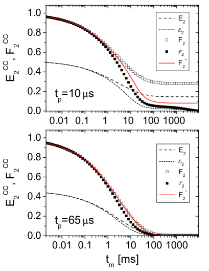
Figure 12: Calculated cos-cos correlation functions for $t_{p}\!=\!10\mathrm{\,\mu s}$ and $t_{p}\!=\!65\mathrm{\,\mu s}$. For the calculations, we utilized Eqs. (II.2) and (11), where $\phi_{y}(t_{m};t_{p})\!=\!\exp[-(t_{m}/3\mathrm{\,ms})^{0.45}]$, $R_{2,y}(2t_{p})\!=\!1$, $R_{1,M}(t_{m})\!=\!\exp(-t_{m}/10\mathrm{\,ms})$ and $R_{1,B}(t_{m})\!=\!\exp(-t_{m}/3\mathrm{\,s})$. The values of the initial and the final correlations were computed for $\delta_{B}\!=\!2\pi\!\times\!120\mathrm{\,kHz}$ and $\delta_{M}\!=\!2\pi\!\times\!40\mathrm{\,kHz}$ according to Eqs. (9) and (10). We show the correlation functions $E_{2}^{CC}(t_{m};t_{p})$ and ${\cal E}_{2}^{CC}(t_{m};t_{p})$, differing due to the action of SLR, together with the normalized counterparts $F_{2}^{CC}(t_{m};t_{p})$ and ${\cal F}_{2}^{CC}(t_{m};t_{p})$. Moreover, we include the correlation functions $F_{2}^{*}(t_{m};t_{p})$ calculated according to Eq. (12).

To make the effects more clear, we show several calculated correlation functions in Fig. 12. For the calculation, we assume that the molecular rotational jumps are described by a KWW function $\phi(t_{m})\!=\!\exp[-(t_{m}/3\mathrm{ms})^{0.45}]$. Further, $\delta_{B}\!=\!2\pi\!\times\!120\mathrm{\,kHz}$ and $\delta_{M}\!=\!2\pi\!\times\!40\mathrm{\,kHz}$ are used to compute the initial and the residual correlations. Utilizing these data, $E_{2}^{CC}$ is obtained from Eq. (II.2). To mimic the damping due to SLR, we calculate ${\cal E}_{2}^{CC}$ according to Eq. (11). In doing so, we suppose exponential relaxation functions $R_{1,y}(t_{m})$ characterized by $T_{1,M}\!=\!10\mathrm{\,ms}$ and $T_{1,B}\!=\!3\mathrm{\,s}$. Thus, the decays due to dynamics and relaxation interfere for the M deuterons. In Fig. 12, the effect of SLR is evident from comparison of $E_{2}^{CC}$ and ${\cal E}_{2}^{CC}$. Normalizing these data, we obtain $F_{2}^{CC}$ and ${\cal F}_{2}^{CC}$. Finally, Eq. (12) is used to compute $F_{2}^{*}$. If our approach enables elimination of SLR effects, $F_{2}^{*}(t_{m})$ and $F_{2}^{CC}(t_{m})$ will be identical.

In Fig. 12, we compare the various correlation functions for the evolution times $t_{p}\!=\!10\mathrm{\,\mu s}$ and $t_{p}\!=\!65\mathrm{\,\mu s}$. For the latter evolution time, the condition $z_{B}^{CC}\!=\!z_{M}^{CC}\!\approx\!0$ is met, see Fig. 1, so that elimination of relaxation effects should be possible. This expectation is confirmed by the nice agreement of $F_{2}^{*}(t_{m})$ and $F_{2}^{CC}(t_{m})$. By contrast, for $t_{p}\!=\!10\mathrm{\,\mu s}$, we find $z_{M}^{CC}\!>\!z_{B}^{CC}\!>\!0$. Then, $F_{2}^{*}(t_{m})$ clearly differs from $F_{2}^{CC}(t_{m})$, indicating that correction for SLR is not successful. In particular, $F_{2}^{*}(t_{m})$ exhibits a residual correlation $z_{B}^{CC}/a_{B}^{CC}$, which deviates substantially from the value resulting in the absence of relaxation effects, see Eq. (14).

For an experimental determination of the effective SLR function, we measure the SLR using the saturation recovery technique, where the longitudinal magnetization is read out with a solid-echo so that SSR reduces the height of the solid-echo. For an evolution time $t_{p}$ in the SE experiment, we perform a concomitant SLR experiment choosing the solid-echo delay $t_{e}$ such that the total time intervals during which transversal magnetization exists are equal in both measurement. In detail, we use $t_{e}\!=\!t_{p}$ or $t_{e}\!=\!t_{p}\!+\!\Delta$, depending on whether a three-pulse or a four-pulse sequence is applied in the SE experiment, see Sec. III. Then, in both the SLR and the SE experiment, the contribution of each deuteron species is proportional to the ”effective” magnetization $m_{y}R_{2,y}(2t_{e})$. In particular, the recovery of the longitudinal magnetization is the sum of the contributions $m_{y}R_{2,y}(2t_{e})R_{1,y}(t_{m})$. Multiplication of these contributions with the respective theoretical values of $a_{y}^{CC}(t_{p})$ yields the effective SLR function.

At the studied temperatures, the recovery of the longitudinal magnetization occurs in two steps, which can be attributed to the B and the M deuterons, respectively.Vogel Therefore, it is straightforward to determine the relaxation functions $R_{1,y}(t_{m})$ and the relative contributions of the two deuteron species. When we study the dependence of $F_{2}^{CC}(t_{m};t_{p})$ on the evolution time and, hence, when we use various solid-echo delays $t_{e}\!=\!t_{p}\!+\!\Delta$ in the concomitant SLR measurements, we find that $R_{1,y}(t_{m})$ does not exhibit a systematic variation with $t_{e}$, as one would expect. Therefore, we use the average values for the calculation of the effective SLR functions. However, the relative amplitudes of the two steps depend on the echo delay, indicating that the B and the M deuterons show different SSR behavior. For PPO at $T\!=\!222\mathrm{\,K}$, the contribution of the M deuterons increases from 55% for $t_{e}\!=\!25\mathrm{\mu s}$ to 65% for $t_{e}\!=\!85\mathrm{\mu s}$. Hence, the M deuterons exhibit slower SSR, consistent with a smaller anisotropy parameter $\delta$. When extending the evolution time in SE experiments, this discrepancy in SSR means that the relative contribution of the B deuterons decreases with respect to the theoretical value, $a_{B}^{x}/(a_{B}^{x}\!+\!a_{M}^{x})$.

- (1) N. G. McCrum, B. E. Read and G. Williams, Anelasic and Dielectric Effects in Polymer Solids, Wiley, New York (1967)
- (2) J. D. Ferry, Viscoelastic Properties of Polymers, Wiley, New York (1980)
- (3) K. Schmidt-Rohr and H. W. Spiess, Multidimensional Solid-State NMR and Polymers, Academic Press, London (1994)
- (4) M. J. Duer, Ann. Rep. NMR Spectrosc. 43, 1 (2000)
- (5) R. Böhmer, G. Diezemann, G. Hinze and E. Rössler, Prog. Nucl. Magn. Reson. Spectrosc. 39, 191 (2001)
- (6) R. Böhmer and F. Kremer, in Broadband Dielectric Spectroscopy, eds. F. Kremer and A. Schönhals, Springer, Berlin (2002)
- (7) E. R. deAzevedo, T. J. Bonagamba and D. Reichert, Prog. Nucl. Magn. Reson. Spectrosc. 47, 137 (2005)
- (8) S. Wefing, S. Kaufmann and H. W. Spiess, J. Chem. Phys. 89, 1234 (1988)
- (9) S. Kaufmann, S. Wefing, D. Schaefer and H. W. Spiess, J. Chem. Phys. 93, 197 (1990)
- (10) U. Pschorn, E. Rössler, H. Sillescu, S. Kaufmann, D. Schaefer and H . W. Spiess, Macromolecules 24, 398 (1991)
- (11) D. Schaefer and H. W. Spiess, J. Chem. Phys. 97, 7944 (1992)
- (12) H. W. Spiess, J. Chem. Phys. 72, 6755 (1980)
- (13) R. M. Diehl, F. Fujara and H. Sillescu, Europhys. Lett. 13, 257 (1990)
- (14) E. Rössler and P. Eiermann, J. Chem. Phys. 100, 5237 (1994)
- (15) B. Geil, F. Fujara and H. Sillescu, J. Magn. Reson. 130, 18 (1998)
- (16) G. Hinze, Phys. Rev. E 57, 2010 (1998)
- (17) R. Böhmer and G. Hinze, J. Chem. Phys. 109, 241 (1998)
- (18) U. Tracht, A. Heuer and H. W. Spiess, J. Chem. Phys. 111, 3720 (1999)
- (19) J. Leisen, K. Schmidt-Rohr and H. W. Spiess, J. Non-Cryst. Solids 172-174, 737 (1994)
- (20) A. Heuer, J. Leisen, S. C. Kuebler and H. W. Spiess, J. Chem. Phys. 105, 7088 (1996)
- (21) S. C. Kuebler, A. Heuer and H. W. Spiess, Macromolecules 29, 7089 (1996)
- (22) F. M. Gray, Solid Polymer Electrolytes, VCH, New York (1991)
- (23) M. B. Armand, J. M. Chabagno and M. J. Duclot, in Fast Ion Transport in Solids, eds. P. Vasishta, J. N. Mundy and G. K Shenoy, North-Holland, Amsterdam (1979)
- (24) M. A. Ratner, in Polymer Electrolyte Reviews 1, eds. J. R. MacCallum and C. A. Vincent, Elsevier, London (1987)
- (25) T. Furukawa, Y. Mukasa, T. Suzuki and K. Kano, J. Polym. Sci., Part B 40, 613 (2002)
- (26) M. G. McLin and C. A. Angell, J. Phys. Chem. 95, 9464 (1991)
- (27) J. Moacanin and E. F. Cuddihy, J. Polym. Sci., Part C 14, 313 (1966)
- (28) C. Vachon, M. Vasco, M. Perrier and J. Prud’homme, Macromolecules 26, 4023 (1993)
- (29) C. Vachon, C. Labreche, A. Vallee, S. Besner, M. Dumont and J. Prud’homme, Macromolecules 28, 5585 (1995)
- (30) R. Bergman, A. Brodin, D. Engberg, Q. Lu, C. A. Angell and L. M. Torell, Electrochim. Acta 40, 2049 (1995)
- (31) P. Carlsson, B. Mattsson, J. Swenson, L. M. Torell, M. Käll, L. Börjesson, R. L. McGreevy, K. Mortensen and B. Gabrys, Solid State Ionics 113-115, 139 (1998)
- (32) P. Carlsson, R. Zorn, D. Andersson, B. Farago, W. S. Howells and L. Börjesson, J. Chem. Phys. 114, 9645 (2001)
- (33) P. Carlsson, D. Andersson, J. Swenson, R. L. McGreevy, W. S. Howells and L. Börjesson, J. Chem. Phys. 121, 12026 (2004)
- (34) S. H. Chung, K. R. Jeffrey and J. R. Stevens, J. Chem. Phys. 94, 1803 (1991)
- (35) S. H. Chung, K. R. Jeffrey and J. R. Stevens, J. Chem. Phys. 108, 3360 (1998)
- (36) K. J. Adamic, S. G. Greenbaum, K. M. Abraham, M. Alamgir, M. C. Wintersgill and J. J. Fontanella, Chem. Mater. 3, 534 (1991)
- (37) J. Fan, R. F. Marzke, E. Sanchez and C. A. Angell, J. Non-Cryst. Solids 172-174, 1178 (1994)
- (38) J. P. Donoso, T. J. Bonagamba, P. L. Frare, N. C. Mello, C. J. Magon and H. Panepucci, Electrochim. Acta 40, 2361 (1995)
- (39) M. Forsyth, D. R. MacFarlane, P. Meakin, M. E. Smith and T. J. Bastow, Electrochim. Acta 40, 2343 (1995)
- (40) C. Roux, W. Gorecki, J.-Y. Sanchez, M. Jeannin and E. Belorizky, J. Phys.: Condens. Matter 8, 7005 (1996)
- (41) C. A. Vincent, Electrochim. Acta 40, 2035 (1995)
- (42) S. Arumugam, J. Shi, D. P. Tunstall and C. A. Vincent, J. Phys.: Condens. Matter 5, 153 (1993)
- (43) I. M. Ward, N. Boden, J. Cruickshank and S. A. Leng, Electrochim. Acta 40, 2071 (1995)
- (44) H.-M. Kao, S.-W. Chao and P.-C. Chang, Macromolecules 39, 1029 (2006)
- (45) M. Vogel and T. Torbrügge, J. Chem. Phys. (in press)
- (46) R. Böhmer, T. Jörg, F. Qi and A. Titze, Chem. Phys. Lett. 316, 419 (2000)
- (47) F. Qi, T. Jörg and R. Böhmer, Solid State Nucl. Magn. Reson. 22, 484 (2002)
- (48) S. Wong, R. A. Vaia, E. P. Giannelis and D. B. Zax, Solid State Ionics 86-88, 547 (1996)
- (49) F. Fujara, S. Wefing and H. W. Spiess, J. Chem. Phys. 84, 4579 (1986)
- (50) F. Fujara, W. Petry, W. Schnauss and H. Sillescu, J. Chem. Phys. 89, 1801 (1988)
- (51) A. M. Wachner and K. R. Jeffrey, J. Chem. Phys. 111, 10611(1999)
- (52) M. Vogel and E. Rössler, J. Chem. Phys. 114, 5802 (2001)
- (53) M. Vogel, P. Medick and E. Rössler, Ann. Rep. NMR Spectrosc. 56, 231 (2005)
- (54) Since we focus on nomalized correlation functions in the experimental part, we disregard the usual factor in Eq. (2). This allows us a combined discussion of and .
- (55) J. E. Anderson, Faraday Symp. Chem. Soc. 6, 82 (1972)
- (56) R. Böhmer, J. Magn. Reson. 147, 78 (2000)
- (57) D. Schaefer, J. Leisen and H. W. Spiess, J. Magn. Reson. A 115, 60 (1995)
- (58) D. L. Sidebottom and G. P. Johari, J. Pol. Sci., Part B 29, 1215 (1991)
- (59) C. Leon, K. L. Ngai and C. M. Roland, J. Chem. Phys. 110, 11585 (1999)
- (60) M. Vogel and E. Rössler, J. Magn. Reson. 147, 443 (2000)
- (61) L. M. Torell and S. Schantz, J. Non-Cryst. Solids 131-133, 981 (1991)
- (62) R. Böhmer, J. Non-Cryst. Solids 172-174, 628 (1994)