Reentrant Synchronization and Pattern Formation in Pacemaker-Entrained Kuramoto Oscillators

Abstract

We study phase entrainment of Kuramoto oscillators under different conditions on the interaction range and the natural frequencies. In the first part the oscillators are entrained by a pacemaker acting like an impurity or a defect. We analytically derive the entrainment frequency for arbitrary interaction range and the entrainment threshold for all-to-all couplings. For intermediate couplings our numerical results show a reentrance of the synchronization transition as a function of the coupling range. The origin of this reentrance can be traced back to the normalization of the coupling strength. In the second part we consider a system of oscillators with an initial gradient in their natural frequencies, extended over a one-dimensional chain or a two-dimensional lattice. Here it is the oscillator with the highest natural frequency that becomes the pacemaker of the ensemble, sending out circular waves in oscillator-phase space. No asymmetric coupling between the oscillators is needed for this dynamical induction of the pacemaker property nor need it be distinguished by a gap in the natural frequency.

I Introduction

Synchronization in the sense of coordinated behavior in time is essential for any efficient organization of systems, natural as well as artificial ones. In artificial systems like factories the sequence of production processes should be synchronized in a way that time-and space consuming storage of input or intermediate products is avoided. The same applies to natural systems like networks of cells which obviously perform very efficiently in fulfilling a variety of functions and tasks. In a more special sense, the synchronized behavior refers to oscillators with almost identical individual units, in particular to phase oscillators with continuous interactions as described by the Kuramoto model kurabook . These sets of limit-cycle oscillators describe synchronization phenomena in a wide range of applications kuraothers . One of these applications is pattern formation in chemical oscillatory systems kuranakao , described by reaction-diffusion systems. A well-known example for such a chemical system is the Belousov-Zabotinsky reaction, a mixture of bromate, bromomalonic acid and ferroin, which periodically changes its color corresponding to oscillating concentrations of the red, reduced state and the blue, oxidized state. In these systems, expanding target-like waves and rotating spiral waves are typical patterns zaikin . As Kuramoto showed (as e.g. in kurabook ), these dynamical systems can be well approximated by phase oscillators if the interaction is weak. For reaction-diffusion equations with a nonlinear interaction term he predicted circular waves with strong similarities to the experimental observation of target patterns. In these systems, defects or impurities seem to play the role of pacemakers, driving the system into a synchronized state. Therefore he treated pacemakers as local ”defect” terms leading to heterogeneities in the reaction-diffusion equations.

In this paper we consider two types of pacemakers. In the first part they are introduced as ”defects” in the sense that they have a different natural frequency from the rest of the system, whose oscillators have either exactly the same frequency or small random fluctuations about some common average by assumption, where in the second case the pacemaker’s frequency is clearly different from the values of a typical fluctuation. Actually, we will not consider the latter case, since small fluctuations do not lead to any qualitative change. The ad-hoc distinction of the pacemaker may reflect natural and artificial systems with built-in impurities like those in the Belousov-Zhabotinsky system. We have recently studied these systems for nearest neighbor interactions hmo1 and regular networks in $d$ dimensions for periodic and open boundary conditions. For such systems we have shown that it is the mean distance of all other nodes from the pacemaker (the so-called depth of the network) that determines its synchronizability. Periodic boundary conditions facilitate synchronization as compared to open boundary conditions. Here we extend these results to larger interaction range. The effect of an extended interaction range on oscillatory systems without pacemaker were considered in rogers . We analytically derive the entrainment frequency for arbitrary interaction range between next-neighbor and all-to all interactions. We derive the entrainment window for all- to-all couplings analytically, for intermediate couplings numerically. The entrainment window depends non-monotonically on the interaction range, so that the synchronization transition is reentrant. In our system the reentrance can be explained in terms of the weight of the interaction term and the normalization of the coupling strength.

In the second part we consider a system of oscillators without a ”defect”, all oscillators on the same footing up to the difference in their natural frequencies. An obvious choice for the natural frequencies would be a Gaussian distribution or another random distribution to describe fluctuations in natural frequencies in otherwise homogeneous systems, without impurities. Such systems have been studied by Blasius and Tönjes blasius for a Gaussian distribution. The authors showed that in this case an asymmetric interaction term is needed to have synchronization, this time driven by a dynamically established pacemaker, acting as a source of concentric waves. This result shows that conditions exist under which a system establishes its own pacemaker in a ”self-organized” way. In contrast to the random distribution of natural frequencies we are interested in a (deterministic) gradient distribution, in which the natural frequencies linearly decrease over a certain region in space. Such a deterministic gradient alone is probably not realistic for natural systems, but considered as a subsystem of a larger set of oscillators with natural frequency fluctuations it may be realized over a certain region in space. Here we suppress the fluctuations and focus on the effect of the gradient alone. As it turns out, the asymmetry in the natural frequency distribution is sufficient for creating a pacemaker as center of circular waves in oscillator-phase space, without the need for an asymmetric term in the interaction. The oscillator with the highest natural frequency becomes the source of circular waves in the synchronized system. We call it dynamically induced as its only inherent difference is its local maximum at the boundary in an otherwise ”smooth” frequency distribution. The type of pattern created by the pacemaker has the familiar form of circular waves. Beyond a critical slope in the natural frequencies, full synchronization is lost. It is first replaced by partial synchronization patterns with bifurcation in the frequencies of synchronized clusters, before it gets completely lost for too steep slopes.

The outline of the paper is as follows. In the first part we treat the pacemaker as defect and derive the common entrainment frequency for arbitrary interaction range and topology (section II). Next we determine the entrainment window, analytically for all-to all coupling and numerically for intermediate interaction range (section II). Here we see the reentrance of the transition as a function of the interaction range (section II). In the second part (section III) we consider dynamically induced pacemakers, first without asymmetric interaction term, for which we analytically derive the synchronization transition as a function of the gradient in the frequencies (sections III.1). In section III.2 we add an asymmetric term, so that the pattern formation is no longer surprising due to the results of blasius , but the intermediate patterns of partial synchronization are different. In section IV we summarize our results and conclusions.

II Pacemaker as defect in the system

The system is defined on a network, regular or small-world like. To each node $i$, $i=0,\ldots,N$, we assign a limit-cycle oscillator, characterized merely by its phase $\varphi_{i}$, which follows the dynamics

$$\dot{\varphi}_{i}=\omega+\delta_{i,s}\Delta\omega+\frac{K}{k_{i}}\sum_{j\not=i}A_{j,i}\sin{\left(\varphi_{j}-\varphi_{i}\right)}\;,$$ (1)

with the following notations. The frequency $\omega$ denotes the natural frequencies of the system. In this system we treat the pacemaker as a defect. It is labelled by $s$ and has a natural frequency that differs by $\Delta\omega$ from the frequency of the other oscillators having all the same frequency $\omega$. $\delta_{i,j}$ denotes the Kronecker delta. The constant $K>0$ parameterizes the coupling strength. We consider regular networks and choose

$$A_{j,i}=r^{-\alpha}_{j,i}\;,$$

$r_{j,i}$ the distance between nodes $j$ and $i$, that is

$$r_{j,i}=\min\left(\left[\;|j-i|\;,\;(N+1)-|j-i|\;\right]\right)$$ (2)

on a one-dimensional lattice with periodic boundary conditions. In two or higher dimensions it is the shortest distance in lattice links. The parameter $0\leq\alpha\leq\infty$ tunes the interaction range. Alternatively we consider $A_{j,i}$ as the adjacency matrix on a small-world topology: $A_{j,i}=1$ if the nodes $j$ and $i$ are connected and $A_{j,i}=0$ otherwise). Moreover, $k_{i}=\sum_{j}A_{j,i}$ is the degree of the $i$-th node, it gives the total number of connections of this node in the network. This system was considered before in hmo1 for nearest-neighbor interactions ($\alpha\to\infty$) on a $d$-dimensional hypercubic lattice and on a Cayley tree. Here we extend the results to long-range interactions via $0\leq\alpha<\infty$.

Entrainment frequency and entrainment window

In the appendix of hmo1 we derived the common entrainment frequency $\Omega$ in the phase-locked state, for which $\dot{\varphi}_{i}\equiv\Omega$ for all $i$, to be given as

$$\Omega\;=\;\Delta\omega\frac{k_{s}}{\sum_{i}k_{i}}$$ (3)

in the rotated frame, in which the natural frequency $\omega$ is zero. In particular such a result is obtained directly from system (1), applying the transformation to the rotating frame $\varphi_{i}\to\varphi_{i}+\omega t$ $\forall i$, multiplying the $i$-th equation by $k_{i}$, summing over all equations and then using the fact that $\sum_{i}\sum_{j}A_{j,i}\sin{(\varphi_{j}-\varphi_{i})}=0$, because the symmetry of the adjacency matrix $A$ and the antisymmetry of the $\sin$-function. Whenever $k_{i}\equiv k$ is independent of $i$ as it happens for periodic boundary conditions and homogeneous degree distributions, in particular for $\alpha=0$ (all-to-all coupling), the common frequency (in the non-rotated frame) is given by

$$\Omega\;=\;\frac{\Delta\omega}{N+1}\;+\;\omega\;,$$

independent on $\alpha$. In the limit $N\rightarrow\infty$ the system synchronizes at $\omega$.
Analytical results for the entrainment window were derived for open and periodic boundary conditions and $\alpha\rightarrow\infty$ in hmo1 . For $\alpha=0$, the result is the same as for $\alpha\rightarrow\infty$, periodic boundary conditions and $d\geq 1$

$$\left|\frac{\Delta\omega}{K}\right|_{c}\;=\;\frac{1}{N}+1\;\;\;.$$ (4)

This is seen as follows. Since for all-to-all couplings the mean-field approximation becomes exact, it is natural to rewrite the dynamical equations (1) in terms of the order parameter $Re^{i\psi}$ defined according to

$$R\;e^{i\psi}\;=\;\frac{1}{N}\sum_{j\not=s}e^{i\varphi_{j}}\;.$$

This quantity differs from the usual order parameter just by the fact that the sum runs over $j\not=s$. Eq.s(1) then take the form

$$\begin{array}[]{ll}\Omega=\Delta\omega\;+\;K\;R\;\sin(\psi-\varphi_{s})&\textrm{ , for }i=s\\ \Omega=\frac{K}{N}\sin(\varphi_{s}-\varphi_{i})\;+\;K\;R\;\sin(\psi-\varphi_{i})&\textrm{ , }\forall\;i\not=s\end{array}\;,$$ (5)

Using $\varphi_{i}=\psi$ for all $i\not=s$ as one of the possible solutions and the fact that the $\sin$-function is bounded, these equations imply the entrainment window as given by (4) with $N$ the total number of nodes minus $1$. As we have shown in hmo1 , the same dependence in terms of $N$ holds for a $d$-dimensional hypercubic lattice with $N^{\prime}$ nodes per side and nearest neighbor couplings, for which $N=(N^{\prime}+1)^{d}-1$, so that the entrainment window for nearest neighbor interactions and on a regular lattice decays exponentially with the depth of the network in the limit of infinite dimensions $d$ ; for random and small-world networks the same type of decay was derived in kori .

The intermediate interaction range $0<\alpha<\infty$ cannot be treated analytically. Here the numerical integration of the equations (1) (via a fourth-order Runge-Kutta algorithm with time step $dt=0.05$ and homogeneous initial conditions) shows that the entrainment window is even smaller than in the limiting cases $\alpha=0$ or $\alpha=\infty$ for otherwise unchanged parameters (that is fixed size $N$, dimension $d$, coupling $K$). For these cases formula (4) gives an upper bound on the entrainment window, as one can easily see from Eq.1 for $i=s$ because $\sum_{j\neq s}\sin{(\varphi_{j}-\varphi_{s})}/r_{j,s}^{\alpha}\leq\sum_{j\neq s}1/r_{j,s}^{\alpha}=k_{s}$ , $\forall\alpha$. Actually the entrainment window becomes smaller for intermediate interaction range, a feature leading to the reentrance of the synchronization transition as function of $\alpha$, as we shall see in the figures 1 and 2 below.

Reentrance of the phase transition

Reentrance phenomena are observed in a variety of phase transitions, ranging from superconductor-insulator transitions as function of temperature vanotterlo and noise-induced transitions castro1995 to chaotic coupled-map lattices as function of the coupling anteneodo . In kampf a reentrance phenomenon is discussed as an artifact of the approximation. Reentrance of phase transitions is challenging as long as it appears counterintuitive. For example, it is counterintuitive when synchronization is first facilitated for increasing coupling and later gets blocked when the coupling exceeds a certain threshold, so that synchronization depends non-monotonically on the coupling. As we see in Fig. 1 for a one-dimensional system with periodic boundary conditions and for various system sizes $N$, the entrainment window $|\Delta\omega/K|_{c}$ depends non-monotonically on the interaction range, parameterized by $\alpha$. This dependence is easily explained by looking at the total weight coming from the sum of interactions. This contribution depends non-monotonically on $\alpha$, as $\sum_{j}\sin(\phi_{j}-\phi_{i})/r_{j,i}^{\alpha}$ decreases for increasing $\alpha$, while the coupling strength increases under the same change of $\alpha$, so that there is a competition between the two factors leading to a minimum of the weight for a certain value of $\alpha$. In contrast, if we scale the coupling strength by a constant factor $K/N$, independently of the degree of the node $i$, the overall weight of the sum decreases for increasing $\alpha$ and along with this, the drive to the synchronized state. As it is shown in the inset of Fig. 1, the threshold monotonically decreases with $\alpha$ if the coupling strength is normalized by $1/N$ independently of the actual degree, as expected from our arguments above. The second inset shows the $N$-dependence of the value of $\alpha$ for which synchronization is most difficult to achieve, it converges to $\alpha=3$ for large $N$. Similar non-monotonic behavior is observed if the interaction range is tuned via the number $k$ of nearest neighbors on a ring rather than via $\alpha$, see Fig. 2A and for a small-world topology watts , see Fig. 2B. Here the small-world is constructed by adding random shortcuts with probability $p$ from a regular ring with nearest neighbor interactions ($p=0$) to an all-to-all topology ($p=1$) newman .

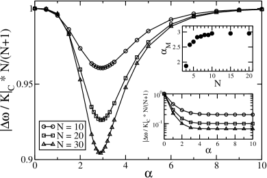
Figure 1: Normalized entrainment window as function of the interaction range parameterized via $\alpha$, for a one-dimensional lattice with $N+1$ sites, periodic boundary conditions and for interaction strength between the oscillators $i$ and $j$ suppressed by the power $\alpha$ of their distance $r_{j,i}$. The main plot indicates the reentrance of the synchronization transition. The upper inset shows the size dependence of $\alpha_{m}$, for which the entrainment window becomes minimal, it saturates at $\alpha\sim 3$. The lower inset shows the monotonic dependence on $\alpha$ for constant coupling strength $K/N$. The figure was obtained for homogeneous initial conditions. The qualitative features remain the same for random initial conditions.

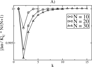
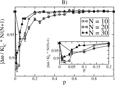
Figure 2: Normalized entrainment window as function of the number of neighbors $k$ (A) and of the probability $p$ for adding shortcuts in a small-world topology (B) for a one-dimensional lattice with periodic boundary conditions and $N+1$ sites. Average values in (B) are taken over $50$ realizations, error bars correspond to the standard deviation. Again the non-monotonic behavior indicates reentrance of the synchronization transition.

III Dynamically induced pacemakers

In view of dynamically induced pacemakers we study the dynamical system

$$\dot{\varphi}_{i}=\omega_{i}+\frac{K}{k_{i}}\sum_{j}A_{j,i}\Gamma(\varphi_{j}-\varphi_{i})\;\;\;,$$ (6)

without a pacemaker. The interaction term $\Gamma$ is given by

$$\Gamma{\left(\varphi_{j}-\varphi_{i}\right)}\;=\;\sin\left(\varphi_{j}-\varphi_{i}\right)\;+\;\gamma\left[1\;-\;\cos\left(\varphi_{j}-\varphi_{i}\right)\right]\;,$$ (7)

where $\gamma=0$ corresponds to antisymmetric interaction, $\gamma>0$ to asymmetric interaction. In the following we consider the cases $\gamma=0$ and $\gamma=2$. The value $\gamma=2$ is chosen for convenience in order of comparing our results with those of Blasius and Tönjes blasius , but different values of $\gamma>0$ lead to qualitatively the same features.
We focus on lattices with periodic boundary conditions in one and two dimensions. Moreover we consider only nearest neighbor interactions, so that in $d=1$ we have $k_{i}=2$ $\forall i$ and $k_{i}=4$ $\forall i$ in $d=2$. The natural frequencies $\omega_{i}$ are chosen from a gradient distribution

$$\omega_{i}=\Delta\omega-r_{i,s}\;\frac{\Delta\omega}{\max_{i}{r_{i,s}}}\;\;\;,$$ (8)

where $r_{i,j}$ is the network distance between the oscillators $i$ and $j$, given by (2) in one dimension and by the shortest path along the edges of the square lattice in two dimensions. The oscillator $s$ is the oscillator with the highest natural frequency. For a one-dimensional lattice with periodic boundary conditions (ring) and $N+1$ oscillators, choosing $s=0$ for simplicity, $\max_{i}{r_{i,0}}=N^{\prime}$, with $N^{\prime}=N/2$ for $N$ even and $N^{\prime}=(N+1)/2$ for $N$ odd. In the following we choose $N$ as even; the case of $N$ odd is very similar.

III.1 Pattern formation for $\gamma=0$

III.1.1 Entrainment frequency

Next we derive the common frequency in case of phase-locking $\dot{\varphi}_{i}\equiv\Omega$ , $\forall i$. Summing the equations of (6) and using the antisymmetry of $\Gamma$ for $\gamma=0$, we obtain

$$\begin{array}[]{l}(N+1)\Omega=\sum_{i=0}^{N}\omega_{i}=\Delta\omega+2\Delta\omega\;\sum_{i=1}^{N/2}\left(1-2i/N\right)=\\ =\Delta\omega\left[1+N-4/N\;\frac{N/2(N/2+1)}{2}\right]=\Delta\omega\frac{N}{2}\;,\end{array}$$

leading to

$$\Omega=\Delta\omega\frac{N}{2(N+1)}\;,$$ (9)

so that $\Omega\;\rightarrow\;\Delta\omega/2$ for $N\rightarrow\infty$.

III.1.2 Entrainment window

It is convenient to rewrite the differential equations (6) in terms of phase lags $\theta_{i}=\varphi_{i}-\varphi_{i-1}$, so that the equation for the oscillator at position $0$ reads

$$\Omega=\omega_{0}+K\sin{(\theta_{1})}\;\Rightarrow\;\sin{(\theta_{1})}=\frac{\Omega-\omega_{0}}{K}\;.$$

For the other oscillators we obtain

$$\begin{array}[]{l}\Omega=\omega_{1}+K/2\left[\sin{(\theta_{2})}-\sin{(\theta_{1})}\right]\\ \Rightarrow\;\sin{(\theta_{2})}=2\frac{\Omega-\omega_{1}}{K}+\sin{(\theta_{1})}\end{array}\;\;\;,$$

$$\begin{array}[]{l}\Omega=\omega_{2}+K/2\left[\sin{(\theta_{3})}-\sin{(\theta_{2})}\right]\\ \Rightarrow\;\sin{(\theta_{3})}=2\frac{\Omega-\omega_{2}}{K}+\sin{(\theta_{2})}\end{array}\;\;\;,$$

so that in general

$$\begin{array}[]{l}\Omega=\omega_{i-1}+K/2\left[\sin{(\theta_{i})}-\sin{(\theta_{i-1})}\right]\\ \Rightarrow\;\sin{(\theta_{i})}=2\frac{\Omega-\omega_{i-1}}{K}+\sin{(\theta_{i-1})}\end{array}$$

or

$$\\ \sin{(\theta_{i})}=\sum_{j=1}^{i-1}\;2\frac{\Omega-\omega_{j}}{K}+\sin{(\theta_{1})}\;.$$

The former sum can be performed as

$$\begin{array}[]{l}\sum_{j=1}^{i-1}\;2\frac{\Omega-\omega_{j}}{K}=\frac{2}{K}\;\sum_{j=1}^{i-1}\left[\Omega-\Delta\omega\left(1-2j/N\right)\right]=\\ =\frac{2}{K}\left(\Omega-\Delta\omega\right)(i-1)+\Delta\omega\frac{2}{K}\frac{i(i-1)}{N}\;,\end{array}$$

from which

$$\sin{(\theta_{i})}=\frac{\Omega-\Delta\omega}{K}\;(2i-1)+\frac{\Delta\omega}{K}\frac{2i^{2}-2i}{N}\;,$$

or, using Eq.(9),

$$\begin{array}[]{l}\sin{(\theta_{i})}=\frac{\Delta\omega}{K}(2i-1)\left[\frac{N}{2(N+1)}-1\right]+\frac{\Delta\omega}{K}\frac{2i(i-1)}{N}=\\ =\frac{\Delta\omega}{K}\;\left[(1-2i)\frac{N+2}{2(N+1)}+\frac{2i(i-1)}{N}\right]\;.\end{array}$$ (10)

For given $N$, we first determine the position $i_{m}$ at which the right-hand-side of Eq.(10) takes its minimum (maximum) value as a function of $i$. This value is constrained by the left-hand-side of (10) to be out of $[-1,1]$. For $i$ treated as a continuous variable the derivative of Eq.(10) with respect to $i$ yields

$$i_{m}=\frac{N(N+2)}{4(N+1)}+\frac{1}{2}\;.$$ (11)

On the other hand

$$i_{m}\geq 1\;\Leftrightarrow N\geq\sqrt{2}\;,$$ (12)

and

$$i_{m}\leq\frac{N}{2}\;\Leftrightarrow\;N\geq 1+\sqrt{3}\;,$$ (13)

so that for $N\gg 1$ , $1\leq i_{m}\leq N/2$ is certainly satisfied. Upon inserting $i_{m}$ from (11) we have

$$\begin{array}[]{l}\left|\frac{\Delta\omega}{K}\right|_{C}=\left|(1-2i_{m})\frac{N+2}{2(N+1)}+\frac{2i_{m}(i_{m}-1)}{N}\right|^{-1}=\\ =\left(\frac{N^{2}(N+2)^{2}+4(N+1)^{2}}{8N(N+1)^{2}}\right)^{-1}\;.\end{array}$$

The critical threshold is then given by

$$\left|\frac{\Delta\omega}{K}\right|_{C}=\frac{8N(N+1)^{2}}{N^{2}(N+2)^{2}+4(N+1)^{2}}\;.$$ (14)

This relation is plotted in Fig. 3, where the full line represents the theoretical prediction, while the full dots correspond to the threshold values, numerically determined by integrating the system of differential Eq.s (6), starting with $N=2$. (The case of $N=2$ violates the constraint (13) in agreement with the fact that for $N=2$ the system degenerates to the former case of having a pacemaker as a defect and two oscillators with natural frequencies $\omega_{1}=\omega_{2}=0$.) Furthermore it should be noticed that Eq.(14) scales as $1/N$ for large values of $N$, the large-$N$ behavior is, however, not visible for the range of $N$, ($N\leq 20$), plotted in Fig. 3.

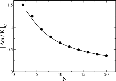
Figure 3: Critical threshold for a one-dimensional lattice as function of its linear size $N$, full line corresponds to the analytic prediction, full dots to numerical results for $N\geq 2$, the symmetry breaking parameter is chosen as $\gamma=0$.

For a ring with maximal distance $N^{\prime}=N/2$ and given $N$ and $K$, the slope $\Delta\omega/N^{\prime}$ in the natural frequencies determines whether synchronization is possible or not. The oscillators synchronize if the values of $N$ lead to a ratio $|\Delta\omega/K|$ below the bound $|\Delta\omega/K|_{C}$ of Eq.(14), named as in section II, Eq.(4), but with $\Delta\omega$ now standing for the maximal difference between the highest and the lowest natural frequencies. If for given $N$ the slope, parameterized by $\Delta\omega$, exceeds this threshold, no entrainment is possible. For $N\rightarrow\infty$ the allowed slope goes to zero, the system does no longer synchronize. To further characterize the synchronization patterns, we measure the stationary frequency $f_{i}$ of the individual oscillators $i$, defined according to

$$f_{i}=\lim_{t\to\infty}\frac{\varphi_{i}(t+t_{0})-\varphi_{i}(t_{0})}{t-t_{0}}\;,$$ (15)

as well as its average $f\;=\;\frac{1}{N+1}\sum_{i=0}^{N}f_{i}$ and variance $\sigma\;=\;\left[\frac{1}{N+1}\sum_{i=0}^{N}\left(f_{i}-f\right)^{2}\right]^{1/2}$. The average frequency and variance are introduced to characterize the intermediate patterns of partial synchronization and to distinguish it from the case $\gamma=2$ in section III.2. In all numerical calculations we set from now on $K=1$. Fig. 4 shows the natural frequencies $(\omega_{i})$ (represented as full line) and the stationary $(f_{i})$ frequencies (shown as dots) for four slopes $\Delta\omega=0.01,0.1,0.2,0.3$, respectively, as function of the position on a linear chain of $100$ oscillators, of which we show only one half due to the symmetric arrangement. The case of $\Delta\omega=0.01$ corresponds to full synchronization, while the other three figures represent partial synchronization of two $(\Delta\omega=0.1)$ and more clusters. It should be noticed that the two clusters for $(\Delta\omega=0.1)$ would violate the condition (14) if they were isolated clusters of $50$ oscillators each with a slope determined by $\Delta\omega=0.1$, but due to the nonlinear coupling to the oscillators of the second cluster, the partial synchronization is a stationary pattern. Fig. 5 displays the frequencies $f_{i}$ as function of the slope, again parameterized by $\Delta\omega$. Here we have chosen $N=20$. We clearly see the bifurcation in frequency space starting at the critical value of $\Delta\omega\simeq 0.36$ and ending with complete desynchronization, in which the stationary frequencies equal the natural frequencies. For frequency synchronization the phases are locked, but their differences to the phase of say the oscillator $s=0$ ($\psi_{i}=\varphi_{i}-\varphi_{0}$) increases nonlinearly with their distance from $s$, as seen in Fig. 6. Therefore the distance between points of the same $\psi$ decreases with $i$.

In two dimensions we simulated $100\times 100$ oscillators on a square lattice with periodic boundary conditions and the oscillator $s$ with the highest natural frequency placed at the center of the square lattice. The natural frequencies of the oscillators are still given by Eq.(8). Their spatial distribution looks like a square pyramid centered at the middle of the square lattice. Fig. 7 displays $\sin\psi_{i}$ on this grid. It exhibits stationary patterns after $2\cdot 10^{4}$ steps of integration, for six choices of $\Delta\omega$, all above the synchronization threshold. We see some remnants of synchronization, most pronounced in Fig. 7A, in which a circular wave is created at the center at $s$, and coexists with waves absorbed by sinks at the four corners of the lattice. The projection of Fig. 7A on one dimension corresponds to Fig. 4B with a bifurcation into two cluster-frequencies. Note that it is again the oscillator with the highest natural frequency that becomes the center of the outgoing wave, while the corners with the lowest natural frequencies $(\omega_{i}=0)$ become sinks. Although Fig. 7F shows almost no remnant of synchronization, it is interesting to follow the time evolution towards this ”disordered” pattern via a number of snapshots, as displayed in Fig. 8 after $9$ [$22.5$] (A), $41$ [$102.5$] (B) , $150$ [$375$] (C) , $393$ [$982.5$] (D), $490$ [$1225$] (E), $1995$ [$4987.5$] (F) integration steps $T$ [$T\;\Delta\omega$ time steps in units of natural frequency($\Delta\omega)$ of Eq.8]. While the pattern of (A) would be stationary in case of full synchronization, here it evolves after iterated reflections to that of (F). The pattern of (F) is stationary in the sense that it stays ”disordered”, on a ”microscopic” scale it shows fluctuations in the phases. The evolution takes a number of time steps, since the interaction is mediated only via nearest neighbors and not of the mean-field type (all-to-all coupling).

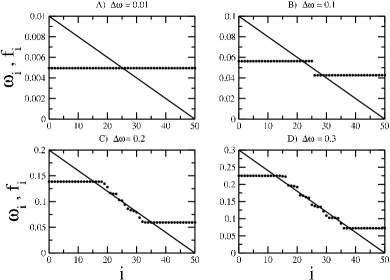
Figure 4: Natural frequencies $\omega_{i}$ (full lines) and measured, stationary frequencies $f_{i}$ (full dots) as function of the position $i$ of the oscillators on a one-dimensional lattice, for $N=100$, periodic boundary conditions, and four values of the maximal natural frequency $\Delta\omega$. The oscillator with maximal natural frequency $\Delta\omega$ is at position $s=0$. Only half of the oscillators up to index $50$ are shown because of the symmetric arrangement. The symmetry breaking parameter is chosen as $\gamma=0$.

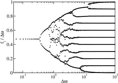
Figure 5: Bifurcation in cluster-frequency space above a critical slope in the natural frequencies, parameterized by $\Delta\omega$, the maximal natural frequency. Numerically measured frequencies $f_{i}$ (normalized such that $f_{i}/\Delta\omega$ $\in$ $[0,1]$) as function of $\Delta\omega$ for a one-dimensional lattice with $N=20$ and periodic boundary conditions. The symmetry breaking parameter is chosen as $\gamma=0$.

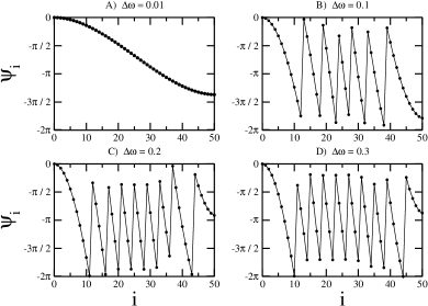
Figure 6: Phase differences $\psi_{i}=\varphi_{i}-\varphi_{0}$ (from the oscillator at $i=0$) as function of the oscillator index $i$ for a one-dimensional lattice, with $N=100$ and periodic boundary conditions, for different values of the maximal natural frequency $\Delta\omega$ and $\gamma=0$. The difference depends nonlinearly on the distance from the oscillator at $i=0$. The “steps” in these plots are due to the projection of the variables $\psi_{i}$ onto the interval $[0,2\pi)$.

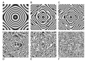
Figure 7: Pattern formation for symmetry breaking parameter $\gamma=0$ on a two-dimensional lattice with $N=100$ oscillators per side. The oscillator $s$ with the maximal natural frequency is placed at the center the lattice. We plot $\sin\psi_{i}$ for every oscillator $i$. The colors vary between white, corresponding to $-1$, and black, corresponding to $1$. The plots are realized after $2\cdot 10^{4}$ integration steps and for different values of $\Delta\omega$ [therefore after different time in natural units of $\Delta\omega$]: A) $0.1$ [$10^{2}$] , B) $0.5$ [$5\cdot 10^{2}$] , C) $1.0$ [$10^{3}$] , D) $5.0$ [$5\cdot 10^{3}$] , E) $10$ [$10^{4}$] , F) $50$ [$5\cdot 10^{4}$]. A cross section through the pattern of A) would reveal a frequency distribution as in Fig.4B.

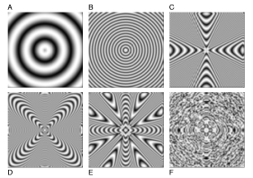
Figure 8: Time evolution of the ”disorder” in Fig. 7F for symmetry breaking parameter $\gamma=0$. All plots are realized for $\Delta\omega=50$, after a different number of integration steps [time in natural units of $\Delta\omega$]: A) $9$ [$22.5$] B) $41$ [$102.5$] , C) $150$ [$375$] , D) $393$ [$982.5$] , E) $490$ [$1225$], F) $1995$ [$4987.5$]. Only the pattern of F) is stationary on a global scale, i.e., up to local fluctuations in the phases.

III.2 Pattern formation for $\gamma=2$

Next let us consider system (6) for $\gamma=2$, for which we expect pattern formation from the results of blasius due to the broken antisymmetry of $\sin$ via a $\cos$-term in the interaction. The main difference shows up in the partial synchronization patterns above the synchronization threshold. As it is evident from Fig.s 9 and 10, the size of the one synchronized cluster, filling the whole lattice below the threshold, shrinks with increasing $\Delta\omega$, since the oscillators with the highest natural frequencies decouple from the cluster, but the remaining oscillators do not organize in other synchronized clusters, the cluster-frequency does no longer bifurcate as before. Along with this, the two-dimensional stationary patterns change to those of Fig. 11, whereas the evolution towards Fig. 11F is now displayed in Fig.s 12 with snapshots taken after $9$ [$22.5$] (A), $48$ [$120$] (B), $160$ [$400$] (C), $277$ [$692.5$] (D), $386$ [$965$] (E), and $2926$ [$7315$] (F) integration steps [$T\;\Delta\omega$ as above].

A further manifestation of the difference in the partial synchronization patterns is seen in the average frequency $f$ and the variance $\sigma$ as function of $\Delta\omega$ (Fig. 13). Above the synchronization transition the average frequency remains constant for $\gamma=0$, but increases for $\gamma=2$ in agreement with Fig.s 9 and 10, the variance increases in both cases ($\gamma=0$ and $\gamma=2$) above the transition, so that it may serve as order parameter. Therefore we can tune the synchronization features via the slope of the gradient.

The main qualitative feature, however, is in common to both systems with and without antisymmetric coupling: the oscillator with the highest natural frequency becomes the center of outgoing circular waves, it is dynamically established as pacemaker. The patterns, seen here in case of full and partial synchronization, are quite similar to those predicted by Kuramoto kurabook for reaction-diffusion systems with continuous diffusion terms, and to those experimentally observed in chemical oscillatory systems zaikin .

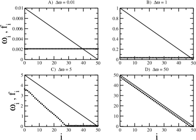
Figure 9: Natural and measured frequencies for symmetry breaking parameter $\gamma=2$. The frequency of the synchronized cluster decreases and the cluster size shrinks, until all oscillators keep their natural frequency in a completely desynchronized state.

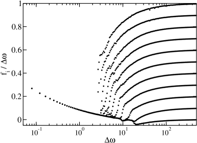
Figure 10: Bifurcation in cluster-frequency for symmetry breaking parameter $\gamma=2$. Above the synchronization threshold the size of the original synchronized cluster shrinks with $\Delta\omega$. Oscillators outside this cluster stay isolated in contrast to Fig. 5.

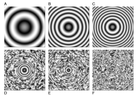
Figure 11: Pattern formation for symmetry breaking parameter $\gamma=2$. We use the same parameter choice as in Fig. 7. Now Fig.s A), B), C) correspond to full synchronization, while one-dimensional cross sections through D), E), and F) would reveal distributions of $f_{i}$ as in Fig.9 C)-D).

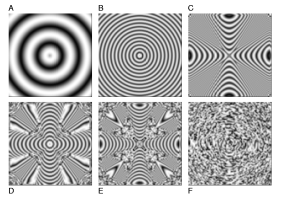
Figure 12: Time evolution for symmetry breaking parameter $\gamma=2$, otherwise same as in Fig. 8. This time the plots are realized after $9$ [$22.5$] (A), $48$ [$120$] (B), $160$ [$400$] (C), $277$ [$692.5$] (D), $386$ [$965$] (E), and $2926$ [$7315$] (F) time steps [time in units of $\Delta\omega$]. Only the disordered pattern of (F) is stationary up to local fluctuations in the phases.

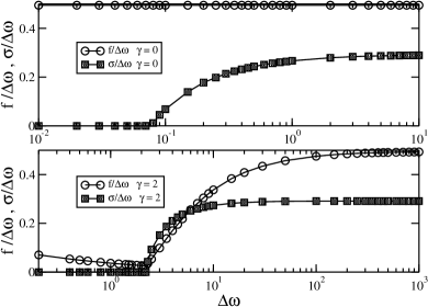
Figure 13: Average frequency and variance as defined in the text (both divided by $\Delta\omega$) as function of the maximal natural frequency $\Delta\omega$, in case of a one-dimensional lattice with $N=100$ oscillators and for values of the symmetry breaking parameter $\gamma=0$ and $\gamma=2$. The raise in the variance from zero indicates the transition to the desynchronized phase.

IV Summary and conclusions

For pacemakers implemented as defect we have extended former results on the entrainment frequency and the entrainment window to arbitrary interaction range, analytically for $\alpha=0$, numerically for intermediate $0<\alpha<\infty$. For large dimensions the entrainment window decays exponentially with the average distance of nodes from the pacemaker so that only shallow networks allow entrainment. The synchronization transition is reentrant as function of $\alpha$ (or $k$, the number of neighbors on a ring, or $p$, the probability to add a random shortcut to the ring topology). The entrainment gets most difficult for $\alpha\sim 3$ and large $N$, while its most easily achieved for next-neighbor and all-to-all couplings. This reentrance is easily explained in terms of the normalization of the coupling strength. For the same system without a pacemaker, but with a gradient in the initial natural frequency distribution the oscillator with the highest natural frequency becomes the center of circular waves, its role as a pacemaker is dynamically induced without the need for an asymmetric term in the interaction. Here we analytically determined the synchronization transition as function of the gradient slope. Above some threshold, full synchronization on one or two-dimensional lattices is lost and replaced by partial synchronization patterns. These patterns depend on the asymmetry parameter $\gamma$. For $\gamma=0$ we observe a bifurcation in frequency space, for $\gamma=2$ the one synchronized cluster shrinks in its size, before for even steeper slopes synchronization is completely lost. For artificial networks these results may be used to optimize the placement and the number of pacemakers if full synchronization is needed, or to control synchronization by tuning the slope of natural frequency gradients.

References

- (1) Y. Kuramoto , ”Chemical Oscillators, Waves, and Turbulence” , (Springer New York 1984).
- (2) A.T. Winfree , ”The geometry of biological time” , (Springer-Verlag New York 1980) ; J. Buck , Nature 211 , 562 (1966) ; T.J. Walker , Science 166 , 891 (1969) ; I. Kanter , W. Kinzel , and E. Kanter , Europhys. Lett. 57 , 141 (2002) ; B. Blasius , A. Huppert, and L. Stone , Nature (London) 399 , 354 (1999) ; J.A. Acebrón , L.L. Bonilla , C.J. Pérez-Vicente , F. Ritort , and R. Spigler , Rev. Mod. Phys. 77 , 137 (2005).
- (3) Y. Kuramoto and H. Nakao, Physica D 103, 294 (1997) ; Y. Kuramoto, D. Battogtokh, and H. Nakao, Phys. Rev. Lett. 81 , 3543 (1998).
- (4) A.N. Zaikin , and A.M. Zhabotinsky , Nature 225 , 535 (1970).
- (5) F. Radicchi, and H. Meyer-Ortmanns, Phys. Rev. E 73 , 036218 (2006).
- (6) J. Rogers , L.T. Wille , Phys. Rev. E 54 , 2192(R) (1996) ; M. Marodi , F. d’Ovidio, and T. Vicsek , Phys. Rev. E 66 , 011109 (2002).
- (7) B. Blasius , and R. Tönjes , Phys. Rev. Lett. 95 , 084101 (2005) ; Y. Kuramoto , and T. Yamada , Prog. Theor. Phys. 56 , 724 (1976).
- (8) H. Kori , and A.S. Mikhailov , Phys. Rev. Lett. 93 , 254101 (2004).
- (9) A. van Otterlo, K.H. Wagenblast , R. Fazio , and G. Schön, Phys. Rev. B 48, 3316 (1993).
- (10) F. Castro , A.D. Sanchez , and H.S. Wio , Phys. Rev. Lett. 75 , 1691 (1995).
- (11) C. Anteneodo , S.E. de S. Pinto , A.M. Batista , and R.L. Viana , Phys. Rev. E 68 , 045202 (2003) ; C. Anteneodo , S.E. de S. Pinto , A.M. Batista , and R.L. Viana , Phys. Rev. E 69 , 029904(R) (2004).
- (12) A.P. Kampf and G. Schön , Physica 152 , 239 (1988); K.B. Efetov, Zh. Eksp. Teor. Fiz. 78 , 2017 (1980).
- (13) D.J. Watts , and S.H. Strogatz , Nature 393 , 440 (1998).
- (14) R. Monasson , Eur. Phys. J. B 12 , 555 (1999) ; M.E.J. Newman , and D.J. Watts , Phys. Lett. A 263 , 341 (1999).