Fermi gas near unitarity around four and two spatial dimensions

Abstract

We construct systematic expansions around four and two spatial dimensions for a Fermi gas near the unitarity limit. Near four spatial dimensions such a Fermi gas can be understood as a weakly interacting system of fermionic and bosonic degrees of freedom. To the leading and next-to-leading orders in the expansion over $\epsilon=4-d$, with $d$ being the dimensionality of space, we calculate the thermodynamic quantities and the fermion quasiparticle spectrum, both at unitarity and around the unitarity point. Then the phase structure of the polarized Fermi gas in the unitary regime is studied in the $\epsilon$ expansion. At unitarity the unpolarized superfluid state and a fully polarized normal state are separated by a first order phase transition. However, on the BEC side of the unitarity point, in a certain range of the two-body binding energy, these two phases are separated in the phase diagram by more exotic phases, including gapless superfluid phases with one or two Fermi surfaces and a superfluid phase with a spatially varying condensate. We also show that the unitary Fermi gas near two spatial dimensions is weakly interacting, and calculate the thermodynamic quantities and the fermion quasiparticle spectrum in the expansion over $\bar{\epsilon}=d-2$.

I Introduction

Two-component Fermi gas with zero-range interaction at infinite scattering length Leggett ; Nozieres , frequently referred to as the unitary Fermi gas, has attracted intense attention across many subfields of physics. Experimentally, the system can be realized in atomic traps using the Feshbach resonance and has been extensively studied OHara ; Jin ; Grimm ; Ketterle ; Thomas ; Salomon ; Thomas05 . Since the fermion density is the only dimensionful scale of the unitary Fermi gas, its properties are universal, i.e., independent of details of the interparticle interaction. The unitary Fermi gas is an idealization of dilute nuclear matter and may be relevant to the physics of neutron stars Bertsch . It has been also suggested that its understanding may be important for high-$T_{\mathrm{c}}$ superconductivity highTc .

The austere simplicity of the unitary Fermi gas implies great difficulties for theoretical treatment, because there seems to be no parameter for a perturbation theory. The usual Green’s function techniques for the many-body problem are completely unreliable here since the expansion parameter $ak_{\mathrm{F}}$ becomes infinite in the unitarity limit. Considerable progress has been made by Monte Carlo simulations Carlson2003 ; Chen:2003vy ; Astrakharchik2004 ; Carlson:2005kg , however these simulations have many limitations, which become especially evident for systems with a population imbalance between two fermion components (finite polarization).

Recently, we have proposed a new approach for the unitary Fermi gas based on the systematic expansion in terms of the dimensionality of space nishida06 , utilizing the specialty of four spatial dimensions in the unitarity limit nussinov04 . In this approach, one would extend the problem to arbitrary spatial dimension $d$ and consider $d$ is close to, but below, four. Then one performs all calculations treating $\epsilon=4-d$ as a small parameter of the perturbative expansion. Results for the physical case of three spatial dimensions are obtained by extrapolating the series expansions to $\epsilon=1$.

We used this $\epsilon$ expansion around four spatial dimensions to calculate thermodynamic quantities and fermion quasiparticle spectrum in the unitarity limit and found results which are quite consistent with those obtained by Monte Carlo simulations and experiments nishida06 . Very recently, this expansion has been successfully applied to atom-dimer and dimer-dimer scatterings in vacuum Rupak:2006jj . Thus there are compelling reasons to hope that the limit $d\to 4$ is not only theoretically interesting but also practically useful, despite the fact that the expansion parameter $\epsilon$ is one at $d=3$. One may hope that the expansion over $4-d$ will be as fruitful for the Fermi gas at unitarity as it has been in the theory of the second order phase transition WilsonKogut .

This paper has four main purposes. We will give a detailed account of the $\epsilon$ expansion for the unitary Fermi gas studied in our recent Letter nishida06 , extend the results to the Fermi gas with large but finite scattering length, study a phase diagram of a polarized Fermi gas near the unitarity limit, and develop a complementary expansion for the unitary Fermi gas around two spatial dimensions.

The structure of the paper is as follows. We start with the study of two-body scattering in vacuum in the unitarity limit for arbitrary spatial dimension $2<d<4$. This study will clarify why systematic expansions around four and two spatial dimensions are possible for the unitary Fermi gas (Sec. II). The $\epsilon$ expansion is developed for an unpolarized Fermi gas both at unitarity and at large, but finite, scattering length in Sec. III. Then we apply the $\epsilon$ expansion to the unitary Fermi gas with unequal densities for the two fermion components. Such a system will be called “polarized” Fermi gas and has been recently realized in experiments Ketterle-polarized ; Hulet-polarized ; Ketterle-polarized2 ; Ketterle-polarized3 . The phase structure of the polarized Fermi gas in the unitary regime is investigated based on the $\epsilon$ expansion in Sec. IV. We also show in Sec. V that there exists a systematic expansion for the Fermi gas in the unitarity limit around two spatial dimensions. In Sec. VI, we make an exploratory discussion to connect the two expansions around four and two spatial dimensions. The summary and concluding remarks are given in Sec. VII.

II Two-body scattering in vacuum

II.1 Qualitative discussion

Nussinov and Nussinov nussinov04 were the first two to recognize the special role of two and four spatial dimensions in the unitarity limit. Their arguments are very simple and we review them here for completeness.

In low dimensions $d\leq 2$, any attractive potential possesses at least one bound state. Therefore, the threshold of the appearance of the first two-body bound state corresponds to the zero coupling. It follows that the Fermi gas in the unitary limit corresponds to a noninteracting Fermi gas at $d\to 2$ and the energy per particle approaches that of the free Fermi gas in this limit. If one defines a parameter $\xi$ as the ratio of the energy density of the Fermi gas at unitarity and that of the free Fermi gas with the same density,

$$\xi=\frac{E}{E_{\mathrm{free}}},$$ (1)

then according to the above argument $\xi\to 1$ as $d\to 2$ from above. (The singular character of $d=2$ was also recognized in the earlier work randeria-2d .)

Now we consider dimensions close to four. At infinite scattering length, the wave function of two fermions with opposite spin behaves like $R(r)=1/r^{d-2}$ at small $r$, where $r$ is the separation between two fermions. Therefore, the normalization integral of the wave function takes the form

$$\int\!d\bm{r}R(r)^{2}=\int_{0}dr\frac{1}{r^{d-3}},$$ (2)

which has a singularity at $r\to 0$ in high dimensions $d\geq 4$. For these dimensions the two-body wave function has infinite probability weight at the origin, and the fermion pair looks like a pointlike boson. From this observation, Nussinov and Nussinov concluded that the unitary Fermi gas at $d\to 4$ becomes a noninteracting Bose gas. In particular, the energy per particle at fixed Fermi energy goes to zero as $d\to 4$, because all bosons condense into the zero energy state and their binding energy is also zero. According to this argument, $\xi\to 0$ as $d\to 4$ from below.

This qualitative observation by Nussinov and Nussinov, however, leaves many questions unanswered:

1. How do the bosons interact with each other?

2. How fast does $\xi$ approach 0 as $d\to 4$?

3. Can one develop a theory based on an expansion over $\epsilon=4-d$?

In order to develop a framework that can be used to answer these questions, we need to review the two-body scattering in a general number of spatial dimension $d$, with special attention to $d$ near four and two, from the perspective of the diagrammatic approach. This consideration will provide a foundation for the construction of systematic expansions for the many-body problem of the unitary Fermi gas.

II.2 Around four spatial dimensions

One can describe the system of spin-$\frac{1}{2}$ fermions with short-range interaction by the following Lagrangian density (here and below $\hbar=1$):

$$\mathcal{L}=\sum_{\sigma=\uparrow,\downarrow}\psi_{\sigma}^{\dagger}\left(i\partial_{t}+\frac{\bm{\nabla}^{2}}{2m}\right)\psi_{\sigma}+c_{0}\,\psi^{\dagger}_{\uparrow}\psi^{\dagger}_{\downarrow}\psi_{\downarrow}\psi_{\uparrow}.$$ (3)

Here $m$ is the fermion mass and $c_{0}$ is the bare attractive coupling between two fermions. The last term in Eq. (3) corresponds to the interaction potential

$$V(\bm{r})=-c_{0}\delta(\bm{r}).$$ (4)

It is well known for $d=3$ that in order to have a finite scattering length, the potential in Eq. (4) has to be regularized: One chooses a particular shape of the potential (for example, the square-well shape), and then takes the width of the potential to be zero simultaneously with adjusting the height so that the zero-energy wave function approaches a finite limit. We shall show that it is true for $d$ between two and four considering the two-body scattering.

The $T$-matrix of the two-body scattering is given by the infinite summation of bubble diagrams. As a result, its inverse is

$$T(p_{0},{\bm{p}})^{-1} =\frac{1}{c_{0}}+i\int\!\frac{dk_{0}\,d{\bm{k}}}{(2\pi)^{d+1}}\frac{1}{\frac{p_{0}}{2}-k_{0}-\varepsilon_{\frac{{\bm{p}}}{2}-{\bm{k}}}+i\delta}$$

$$\qquad\qquad\qquad\times\frac{1}{\frac{p_{0}}{2}+k_{0}-\varepsilon_{\frac{{\bm{p}}}{2}+{\bm{k}}}+i\delta}$$

$$=\frac{1}{c_{0}}-\int_{\bm{k}}\frac{1}{2\varepsilon_{\bm{k}}-p_{0}+\frac{\varepsilon_{\bm{p}}}{2}-i\delta},$$ (5)

where $\varepsilon_{\bm{p}}={\bm{p}}^{2}/2m$ is the kinetic energy of nonrelativistic particles and we introduced the shorthand notation

$$\int_{\bm{k}}\equiv\frac{d{\bm{k}}}{(2\pi)^{d}}.$$ (6)

The integration over ${\bm{k}}$ in Eq. (II.2) is ultraviolet divergent as $\int\!d{\bm{k}}/k^{2}$ if $d>2$ and needs to be regularized.

The usual way to do this regularization is to assume that there is an upper limit $\Lambda$ in the momentum integral of Eq. (II.2), and to adjust the $\Lambda$ dependence of $c_{0}$ so that the physics does not depend on $\Lambda$. If we add and subtract the value of the integral at $p_{0}={\bm{p}}=0$, we have

$$\begin{split}T(p_{0},{\bm{p}})^{-1}&=\frac{1}{c_{0}(\Lambda)}-{\int\limits^{\Lambda}}_{\!\!\!{\bm{k}}}\,\frac{1}{2\varepsilon_{\bm{k}}}\\ &\quad-{\int\limits^{\Lambda}}_{\!\!\!{\bm{k}}}\left(\frac{1}{2\varepsilon_{\bm{k}}-p_{0}+\frac{\varepsilon_{\bm{p}}}{2}-i\delta}-\frac{1}{2\varepsilon_{\bm{k}}}\right).\end{split}$$ (7)

The second integral is now $\int\!d{\bm{k}}/k^{4}$ at large ${\bm{k}}$ and converges for $d<4$. Thus for $d<4$ one can set the cutoff to infinity in the second integral. The first integral is still ultraviolet divergent but is independent of $p_{0}$ and ${\bm{p}}$, and it can be absorbed into the definition of the renormalized coupling $c_{0}^{\mathrm{ren}}$ as follows:

$$\frac{1}{c_{0}^{\mathrm{ren}}}\equiv\frac{1}{c_{0}(\Lambda)}-{\int\limits^{\Lambda}}_{\!\!\!{\bm{k}}}\,\frac{1}{2\varepsilon_{\bm{k}}}.$$ (8)

The zero range limit corresponds to sending $\Lambda\to\infty$ but keeping the renormalized coupling $c_{0}^{\mathrm{ren}}$ finite by an appropriate choice of the bare coupling $c_{0}(\Lambda)$. In this limit all physical quantities should depend only on $c_{0}^{\mathrm{ren}}$ but not on $c_{0}$ and $\Lambda$ separately. From the above discussion it is clear that this limit can be taken only for $d<4$; for $d\geq 4$ the divergences in the fermion loop can no longer be compensated by the renormalization of one coupling constant $c_{0}$. There is no universal zero range and large scattering length limit for $d\geq 4$.

In this paper we will not use the momentum-cutoff regularization described above. Rather we shall use the dimensional regularization, in which the integrals are evaluated in dimensions where they are ultraviolet finite and then the results are analytically continued to the dimension $d$. For example, the integral

$$\int_{\bm{k}}\frac{\varepsilon_{\bm{k}}^{\,m}}{(\varepsilon_{\bm{k}}^{\,2}+\phi_{0}^{\,2})^{n/2}}$$ (9)

converges only for $d+2m<2n$, but we will use the analytical formula

$$\begin{split}&\int_{\bm{k}}\frac{\varepsilon_{\bm{k}}^{\,m}}{(\varepsilon_{\bm{k}}^{\,2}+\phi_{0}^{\,2})^{n/2}}\\ &\quad=\frac{\Gamma\left(\frac{d}{4}+\frac{m}{2}\right)\Gamma\left(\frac{n-m}{2}-\frac{d}{4}\right)}{2\,\Gamma\left(\frac{d}{2}\right)\Gamma\left(\frac{n}{2}\right)}\left(\frac{m\phi_{0}}{2\pi}\right)^{d/2}\phi_{0}^{\,m-n}\end{split}$$ (10)

for all values of $d$. This regularization scheme is particularly convenient because the divergent integral in the formula defining the renormalized coupling $c_{0}^{\mathrm{ren}}$ is zero,

$$\int_{\bm{k}}\,\frac{1}{2\varepsilon_{\bm{k}}}=0\quad\text{in dimensional\ regularization,}$$ (11)

and hence the renormalized coupling is just the bare coupling, $c_{0}^{\mathrm{ren}}=c_{0}$. In other words, in the dimensional regularization the subtraction of the leading divergence of the fermion bubble diagram is implemented automatically. As long as physical quantities are insensitive to the ultraviolet cutoff, which is the case for $d<4$, the results of the dimensional and momentum-cutoff regularizations coincide.

In the dimensional regularization, the integral in Eq. (II.2) vanishes for $p_{0}={\bm{p}}=0$ (scatterings at threshold). Therefore the limit of infinite scattering length where $T(0,\bm{0})=\infty$ corresponds to $c_{0}=\infty$. In this limit the integration over ${\bm{k}}$ in Eq. (II.2) can be evaluated explicitly,

$$T(p_{0},{\bm{p}})^{-1}=-\Gamma\!\left(1-\frac{d}{2}\right)\left(\frac{m}{4\pi}\right)^{\frac{d}{2}}\left(-p_{0}+\frac{\varepsilon_{\bm{p}}}{2}-i\delta\right)^{\frac{d}{2}-1}.$$ (12)

This expression has a pole at $d=4$ originating from the ultraviolet divergence of the ${\bm{k}}$ integration. Thus the $T$-matrix is small when $d$ is close to four and vanishes at $d=4$, indicating that such a limit can be thought of as a noninteracting limit. Substituting $d=4-\epsilon$ and expanding in terms of $\epsilon$, the $T$-matrix near four spatial dimensions becomes

$$iT(p_{0},{\bm{p}})=-\frac{8\pi^{2}\epsilon}{m^{2}}\frac{i}{p_{0}-\frac{\varepsilon_{\bm{p}}}{2}+i\delta}+O(\epsilon^{2}).$$ (13)

From this equation it is clear what is special about $d$ close to four: As the number of dimensions approaches four from below, the two-fermion scattering amplitude has the form of the scattering process that occurs through the propagation of an intermediate boson whose mass is $2m$, as depicted in Fig. 1.

Figure 1: Two-fermion scattering in vacuum in the unitarity limit. The $T$-matrix near four spatial dimensions is expressed by the propagation of the boson with the small effective coupling $g$, while it reduces to a contact interaction with the small effective coupling $\bar{g}^{2}$ near two spatial dimensions.

The propagator of the intermediate boson is

$$D(p_{0},{\bm{p}})=\left(p_{0}-\frac{\varepsilon_{\bm{p}}}{2}+i\delta\right)^{-1},$$ (14)

and the effective coupling of the intermediate boson to the fermion pair is

$$g^{2}=\frac{8\pi^{2}\epsilon}{m^{2}}.$$ (15)

Then the $T$-matrix, to leading order in $\epsilon$, can be written as

$$iT(p_{0},{\bm{p}})\simeq(ig)^{2}iD(p_{0},{\bm{p}}).$$ (16)

It is natural to interpret the intermediate boson as a bound state of the two fermions at threshold, which will be referred to simply as a boson.

An important point is that the effective coupling of the two fermions into the boson $g\sim\epsilon^{1/2}$ is small near four dimensions. This fact indicates the possibility to construct a perturbative expansion for the unitary Fermi gas near four spatial dimensions in terms of the small parameter $\epsilon$.

II.3 Around two spatial dimensions

Similarly, a perturbative expansion around two spatial dimensions is possible. This is because the inverse of the $T$-matrix in Eq. (12) has another pole at $d=2$ and hence the $T$-matrix vanishes in this limit, which indicates that $d=2$ from above is again a noninteracting limit. Substituting $d=2+\bar{\epsilon}$ and expanding in terms of $\bar{\epsilon}$, the $T$-matrix near two spatial dimensions becomes

$$iT(p_{0},{\bm{p}})=i\frac{2\pi}{m}\bar{\epsilon}+O(\bar{\epsilon}^{2}).$$ (17)

If we define the effective coupling at $2+\bar{\epsilon}$ dimensions as

$$\bar{g}^{2}=\frac{2\pi}{m}\bar{\epsilon},$$ (18)

then the $T$-matrix to the leading order in $\bar{\epsilon}$ can be written as

$$iT(p_{0},{\bm{p}})\simeq i\bar{g}^{2}.$$ (19)

We see that the $T$-matrix near two spatial dimensions corresponds to a contact interaction with the small effective coupling $\bar{g}^{2}\sim\bar{\epsilon}$, as depicted in Fig. 1. In this case, the boson propagator $D(p)$ in Eq. (16) is just a constant $-1$. We defer our discussion of the expansion over $\bar{\epsilon}=d-2$ to Sec. V and concentrate on the expansion over $\epsilon=4-d$.

II.4 Binding energy of two-body state

We shall be interested not only in the physics right at the unitarity point, but also in the vicinity of it. In other words, $1/c_{0}$ can be nonzero in the dimensional regularization. The case of $c_{0}<0$ corresponds to the BEC side of the unitarity point, and $c_{0}>0$ corresponds to the BCS side. In order to facilitate an extrapolation to three spatial dimensions, one would like to identify $c_{0}$ with the scattering length. However, this cannot be done directly since the dimensionality of $c_{0}$ changes with the number of dimensions.

One way to circumvent the problem is to parametrize the deviation from the unitarity by the binding energy of the two-body state. Clearly, this method works only on the BEC side of the unitarity point. Fortunately, as we will find in Sec. IV, all interesting exotic phases of the polarized Fermi gas appear on the BEC side of the unitarity limit.

The binding energy $\varepsilon_{\mathrm{b}}$, defined to be positive $\varepsilon_{\mathrm{b}}>0$, is obtained from the location of the pole of the $T$-matrix at zero external momentum: $T(-\varepsilon_{\mathrm{b}},\bm{0})^{-1}=0$. From Eqs. (II.2) and (12), we see the coupling $c_{0}<0$ is related with $\varepsilon_{\mathrm{b}}$ via the following equation:

$$\frac{1}{c_{0}}=\Gamma\!\left(1-\frac{d}{2}\right)\left(\frac{m}{4\pi}\right)^{\frac{d}{2}}\varepsilon_{\mathrm{b}}^{\,\frac{d}{2}-1}.$$ (20)

Near four spatial dimensions, the relationship between $\varepsilon_{\mathrm{b}}$ and $c_{0}$ to the leading order in $\epsilon=4-d$ is given by

$$\frac{1}{c_{0}}\simeq-\frac{\varepsilon_{\mathrm{b}}}{2\epsilon}\left(\frac{m}{2\pi}\right)^{2}.$$ (21)

In three spatial dimensions, the relationship between $\varepsilon_{\mathrm{b}}$ and the scattering length $a=-mc_{0}/4\pi$ becomes $\varepsilon_{\mathrm{b}}=(ma^{2})^{-1}$.

At finite density in general $d$ dimensions, we shall use $\varepsilon_{\mathrm{b}}/\varepsilon_{\mathrm{F}}$ as the dimensionless parameter characterizing the deviation from the unitarity, where $\varepsilon_{\mathrm{F}}$ is the Fermi energy. If we recall that the Fermi energy is related to the Fermi momentum $k_{\mathrm{F}}$ through $\varepsilon_{\mathrm{F}}=k_{\mathrm{F}}^{\,2}/(2m)$, one finds the following relationship holds at $d=3$:

$$\frac{\varepsilon_{\mathrm{b}}}{\varepsilon_{\mathrm{F}}}=\frac{2}{(ak_{\mathrm{F}})^{2}}.$$ (22)

We will use these relations to compare results in the expansion over $\epsilon=4-d$ with the physics in three spatial dimensions.

III Fermi gas near unitarity

III.1 Lagrangian and Feynman rules

Employing the idea of the previous section, we now construct the $\epsilon$ expansion for the Fermi gas near the unitarity limit. We start with the Lagrangian density in Eq. (3) and introduce two chemical potentials $\mu_{\uparrow}$ and $\mu_{\downarrow}$ for the two spin components as follows:

$$\mathcal{L}=\sum_{\sigma=\uparrow,\downarrow}\psi_{\sigma}^{\dagger}\left(i\partial_{t}+\frac{\bm{\nabla}^{2}}{2m}+\mu_{\sigma}\right)\psi_{\sigma}+c_{0}\,\psi^{\dagger}_{\uparrow}\psi^{\dagger}_{\downarrow}\psi_{\downarrow}\psi_{\uparrow}.$$ (23)

After making a Hubbard-Stratonovich transformation, we rewrite the Lagrangian density as

$$\begin{split}\mathcal{L}&=\Psi^{\dagger}\left(i\partial_{t}+\frac{\sigma_{3}\bm{\nabla}^{2}}{2m}+\mu\sigma_{3}+H\right)\Psi\\ &\qquad\qquad\quad-\frac{1}{c_{0}}\phi^{*}\phi+\Psi^{\dagger}\sigma_{+}\Psi\phi+\Psi^{\dagger}\sigma_{-}\Psi\phi^{*},\end{split}$$ (24)

where $\Psi=(\psi_{\uparrow},\psi^{\dagger}_{\downarrow})^{T}$ is a two-component Nambu-Gor’kov field, and $\sigma_{1,2,3}$ and $\sigma_{\pm}=\frac{1}{2}(\sigma_{1}\pm i\sigma_{2})$ are the Pauli matrices. We define the average chemical potential as $\mu=(\mu_{\uparrow}+\mu_{\downarrow})/2$ and the chemical potential difference as $H=(\mu_{\uparrow}-\mu_{\downarrow})/2$.

The ground state at the finite density system (at least when $H=0$) is a superfluid state where $\phi$ condenses: $\langle\phi\rangle=\phi_{0}$ with $\phi_{0}$ being chosen to be real. With that in mind we expand $\phi$ around its vacuum expectation value $\phi_{0}$ as

$$\phi=\phi_{0}+g\varphi,\qquad g=\frac{(8\pi^{2}\epsilon)^{1/2}}{m}\left(\frac{m\phi_{0}}{2\pi}\right)^{\epsilon/4}.$$ (25)

Here we introduced the effective coupling $g\sim\epsilon^{1/2}$ in Eq. (15). The extra factor $\left(m\phi_{0}/2\pi\right)^{\epsilon/4}$ was chosen so that $\varphi$ has the correct dimension of a nonrelativistic field .

We now split the Lagrangian into three parts, $\mathcal{L}=\mathcal{L}_{0}+\mathcal{L}_{1}+\mathcal{L}_{2}$, where

$$\begin{split}\mathcal{L}_{0}&=\Psi^{\dagger}\left(i\partial_{t}+\frac{\sigma_{3}\bm{\nabla}^{2}}{2m}+H+\sigma_{+}\phi_{0}+\sigma_{-}\phi_{0}\right)\Psi\\ &\qquad+\varphi^{*}\left(i\partial_{t}+\frac{\bm{\nabla}^{2}}{4m}\right)\varphi-\frac{\phi_{0}^{\,2}}{c_{0}}\,,\end{split}$$ (26)

$$\begin{split}\mathcal{L}_{1}&=g\Psi^{\dagger}\sigma_{+}\Psi\varphi+g\Psi^{\dagger}\sigma_{-}\Psi\varphi^{*}+\mu\Psi^{\dagger}\sigma_{3}\Psi\\ &\qquad+\left(2\mu-\frac{g^{2}}{c_{0}}\right)\varphi^{*}\varphi-\frac{g\phi_{0}}{c_{0}}\varphi-\frac{g\phi_{0}}{c_{0}}\varphi^{*}\,,\end{split}$$ (27)

$$\mathcal{L}_{2} =-\varphi^{*}\left(i\partial_{t}+\frac{\bm{\nabla}^{2}}{4m}\right)\varphi-2\mu\varphi^{*}\varphi\,.$$ (28)

The Lagrangian density in Eq. (24) does not have the kinetic term for the boson field $\varphi$. We add such a term to $\mathcal{L}_{0}$ and subtract it in $\mathcal{L}_{2}$. Analogously, we add a chemical potential term for $\varphi$ in $\mathcal{L}_{1}$ and subtract it in $\mathcal{L}_{2}$. At first sight, the split (26)–(28) may appear counterintuitive, but it will greatly simplify the organization of the expansion in powers of $\epsilon$.

We shall also see that the condensate $\phi_{0}$ coincides, to the leading order in $\epsilon$, with the energy gap in the fermion quasiparticle spectrum. From Eq. (21), $-g^{2}/c_{0}\simeq\varepsilon_{\mathrm{b}}$ gives the binding energy of the boson to the leading order in $\epsilon$ when $c_{0}$ is negative. Throughout this paper, we consider the vicinity of the unitarity point where $\varepsilon_{\mathrm{b}}\sim\epsilon\phi_{0}$.

The part $\mathcal{L}_{0}$ is the Lagrangian density of noninteracting fermion quasiparticles and bosons with the mass $2m$. The propagators of fermion and boson are generated by $\mathcal{L}_{0}$. The fermion propagator $G$ is a $2\times 2$ matrix,

$$\begin{split}G(p_{0},{\bm{p}})&=\frac{1}{(p_{0}+H)^{2}-E_{\bm{p}}^{\,2}+i\delta}\\ &\qquad\quad\times\begin{pmatrix}p_{0}+H+\varepsilon_{\bm{p}}&-\phi_{0}\\ -\phi_{0}&p_{0}+H-\varepsilon_{\bm{p}}\end{pmatrix},\end{split}$$ (29)

where $E_{\bm{p}}=\sqrt{\varepsilon_{\bm{p}}^{\,2}+\phi_{0}^{\,2}}$ is the excitation energy of the fermion quasiparticle. The boson propagator $D$ is given by the same form as in Eq. (14),

$$D(p_{0},{\bm{p}})=\left(p_{0}-\frac{\varepsilon_{\bm{p}}}{2}+i\delta\right)^{-1}.$$ (30)

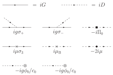
Figure 2: Feynman rules from the Lagrangian density in Eqs. (26)–(28). The two vertices in the last column come from $\mathcal{L}_{2}$, while the rest come from $\mathcal{L}_{1}$. Solid (dotted) lines represent the fermion (boson) propagator $iG$ $(iD)$.

The part $\mathcal{L}_{1}$ generates the vertices depicted in the first two columns of Fig. 2. The first two terms in $\mathcal{L}_{1}$ describe the fermion-boson interactions, whose coupling is proportional to $g\sim\epsilon^{1/2}$ and small in the limit $\epsilon\to 0$. This coupling originates from the two-body scattering in vacuum in the unitarity limit which was studied in the previous section (see Fig. 1). The third and fourth terms are insertions of chemical potentials, $\mu$ and $\mu_{\mathrm{B}}\equiv 2\mu-g^{2}/c_{0}$, to the fermion and boson propagators, respectively. We treat these two insertions as small perturbations for the following reasons. First, we shall see that $\mu$ is small compared to the scale set by $\phi_{0}$, i.e., $\mu/\phi_{0}\sim\epsilon$. Second, we limit ourselves to a region near the unitarity limit where the boson binding energy is small compared to $\phi_{0}$, i.e., $\varepsilon_{\mathrm{b}}/\phi_{0}\sim\epsilon$ so $\mu_{\mathrm{B}}/\phi_{0}\sim\epsilon$. The last two terms in $\mathcal{L}_{1}$ give tadpoles to the $\varphi$ and $\varphi^{*}$ fields, which are proportional to $-ig\phi_{0}/c_{0}$. The condition of cancellation of tadpole diagrams will determine the value of the condensate $\phi_{0}$.

Finally, $\mathcal{L}_{2}$ generates two additional vertices for the boson propagator as depicted in the last column of Fig. 2, which are $-i\Pi_{0}$ and $-2i\mu$ where

$$\Pi_{0}(p_{0},{\bm{p}})=p_{0}-\frac{\varepsilon_{\bm{p}}}{2}.$$ (31)

These two vertices can be thought of as counterterms to avoid double counting of certain types of diagrams which are already taken into $\mathcal{L}_{0}$ and $\mathcal{L}_{1}$. For the rest of this section, we will consider the unpolarized case with $H=0$ at zero temperature.

III.2 Power counting rule of $\epsilon$

We now develop the power counting rule which allows us to identify Feynman diagrams that contribute to a given order in $\epsilon$. Our discussion will extend the power counting scheme developed for the unitarity limit in Ref. nishida06 to the region near the unitarity where $g^{2}/|c_{0}|\sim\epsilon\phi_{0}$.

Let us first consider Feynman diagrams constructed only from $\mathcal{L}_{0}$ and $\mathcal{L}_{1}$, without the vertices from $\mathcal{L}_{2}$. We make a prior assumption $\mu/\phi_{0}\sim\epsilon$, which will be checked later, and consider $\phi_{0}$ to be $O(1)$. Each pair of fermion-boson vertices is proportional to $g^{2}\sim\epsilon$ and hence brings a factor of $\epsilon$. Also, each insertion of $\mu\sim\epsilon$ or ${\mu_{\mathrm{B}}}=2\mu-g^{2}/c_{0}\sim\epsilon$ brings another factor of $\epsilon$. Therefore, the power of $\epsilon$ for a given diagram is naively $N_{g}/2+N_{\mu}$, where $N_{g}$ is the number of couplings $g$ from $\mathcal{L}_{1}$, and $N_{\mu}=N_{{\mu_{\mathrm{F}}}}+N_{{\mu_{\mathrm{B}}}}$ is the sum of the number of $\mu$ insertions to the fermion line and ${\mu_{\mathrm{B}}}$ insertions to the boson line.

However, this naive power counting does not take into account the possibility of inverse powers of $\epsilon$ from loop integrals. Such a $1/\epsilon$ behavior arises for integrals which are ultraviolet divergent at $d=4$. Let us identify diagrams which have this divergence.

Consider a diagram with $L$ loop integrals, $P_{\mathrm{F}}$ fermion propagators, and $P_{\mathrm{B}}$ boson propagators. Each momentum loop integral in the ultraviolet region behaves as

$$\int dp_{0}d{\bm{p}}\sim\int d{\bm{p}}\,\varepsilon_{\bm{p}}\sim p^{6},$$ (32)

while each fermion or boson propagator falls at least as $G(p)\sim p^{-2}$ or $D(p)\sim p^{-2}$ or faster. Therefore, the maximal degree of divergence that the diagram may have is

$$\mathcal{D}=6L-2P_{\mathrm{F}}-2P_{\mathrm{B}}.$$ (33)

We call $\mathcal{D}$ the superficial degree of divergence. $\mathcal{D}=0$ corresponds to the possibility of logarithmic divergence, $\mathcal{D}=2$ to quadratic divergence, etc.

Moreover, following an analysis similar to that done in relativistic field theories Peskin:1995ev , one finds the following relations which involve the number of external fermion (boson) lines $E_{\mathrm{F(B)}}$:

$$\begin{split}L&=(P_{\mathrm{F}}-N_{\mu_{\mathrm{F}}})+(P_{\mathrm{B}}-N_{\mu_{\mathrm{B}}})-N_{g}+1,\\ N_{g}&=(P_{\mathrm{F}}-N_{\mu_{\mathrm{F}}})+\frac{E_{\mathrm{F}}}{2}=2(P_{\mathrm{B}}-N_{\mu_{\mathrm{B}}})+E_{\mathrm{B}}.\end{split}$$ (34)

With the use of these relations, the superficial degree of divergence $\mathcal{D}$ can be written as

$$\mathcal{D}=6-2(E_{\mathrm{F}}+E_{\mathrm{B}}+N_{\mu}),$$ (35)

which shows that the inverse powers of $\epsilon$ appear only in diagrams where the total number of external lines and chemical potential insertions does not exceed three. This is similar to the situation in quantum electrodynamics where infinities occur only in electron and photon self-energies and the electron-photon triple vertex.

However, this estimation of $\mathcal{D}$ is actually an overestimate: for many diagrams the real degree of divergence is smaller than given in Eq. (35). To see that, we split $G(p)$ into the retarded and advanced parts: $G(p)=G^{\mathrm{R}}(p)+G^{\mathrm{A}}(p)$, where $G^{\mathrm{R}}$ ($G^{\mathrm{A}}$) has poles only in the lower (upper) half of the complex $p_{0}$ plane. It is easy to see that the ultraviolet behaviors of different components of the propagators are different:

$$G_{11}^{\mathrm{R}}(p)\sim G_{22}^{\mathrm{A}}(p)\sim D^{\mathrm{R}}(p)\sim p^{-2},\phantom{\sum}$$ (36)

$$G_{12}(p)\sim G_{21}(p)\sim p^{-4},\quad G_{11}^{\mathrm{A}}(p)\sim G_{22}^{\mathrm{R}}(p)\sim p^{-6}.$$

Note that since the boson propagator $D(p)$ has a pole only on the lower half plane of $p_{0}$, we have only the retarded Green’s function for the boson $D^{\mathrm{A}}(p)=0$.

From these analytic properties of the propagators in the ultraviolet region and the vertex structures in $\mathcal{L}_{1}$ as well as the relation of Eq. (35), one can show that there are only four skeleton diagrams which have the $1/\epsilon$ singularity near $d=4$. They are one-loop diagrams of the boson self-energy [Figs. 3(a) and 3(c)], the $\varphi$ tadpole [Fig. 3(e)], and the vacuum diagram [Fig. 3(g)]. We shall examine these apparent four exceptions of the naive power counting rule of $\epsilon$ one by one.

The first diagram, Fig. 3(a), is the one-loop diagram of the boson self-energy. The frequency integral can be done explicitly, yielding

$$\begin{split}-i\Pi_{\mathrm{a}}(p)&=-g^{2}\int\!\frac{dk}{(2\pi)^{d+1}}\,G_{11}\!\left(k+\frac{p}{2}\right)G_{22}\!\left(k-\frac{p}{2}\right)\\ &=ig^{2}\int_{\bm{k}}\frac{1}{4E_{{\bm{k}}-\frac{{\bm{p}}}{2}}E_{{\bm{k}}+\frac{{\bm{p}}}{2}}}\left[\frac{(E_{{\bm{k}}-\frac{{\bm{p}}}{2}}+\varepsilon_{{\bm{k}}-\frac{{\bm{p}}}{2}})(E_{{\bm{k}}+\frac{{\bm{p}}}{2}}+\varepsilon_{{\bm{k}}+\frac{{\bm{p}}}{2}})}{E_{{\bm{k}}-\frac{{\bm{p}}}{2}}+E_{{\bm{k}}+\frac{{\bm{p}}}{2}}-p_{0}-i\delta}+\frac{(E_{{\bm{k}}-\frac{{\bm{p}}}{2}}-\varepsilon_{{\bm{k}}-\frac{{\bm{p}}}{2}})(E_{{\bm{k}}+\frac{{\bm{p}}}{2}}-\varepsilon_{{\bm{k}}+\frac{{\bm{p}}}{2}})}{E_{{\bm{k}}-\frac{{\bm{p}}}{2}}+E_{{\bm{k}}+\frac{{\bm{p}}}{2}}+p_{0}-i\delta}\right].\end{split}$$ (37)

The integral over ${\bm{k}}$ is ultraviolet divergent at $d=4$ and has a pole at $\epsilon=0$. Thus $\Pi_{\mathrm{a}}(p)$ is $O(1)$ by itself instead of $O(\epsilon)$ according to the naive power counting. The residue at the pole is

$$\begin{split}\Pi_{\mathrm{a}}(p)&=-g^{2}\int_{\bm{k}}\left(2\varepsilon_{\bm{k}}-p_{0}+\frac{\varepsilon_{\bm{p}}}{2}\right)^{-1}+\cdots\\ &=-\left(p_{0}-\frac{\varepsilon_{\bm{p}}}{2}\right)+O(\epsilon),\end{split}$$ (38)

and is canceled out exactly by adding the vertex $\Pi_{0}$ in $\mathcal{L}_{2}$. Therefore the diagram of the type in Fig. 3(a), when combined with the vertex from $\mathcal{L}_{2}$ in Fig. 3(b), conforms to the naive $\epsilon$ power counting, i.e., is $O(\epsilon)$.

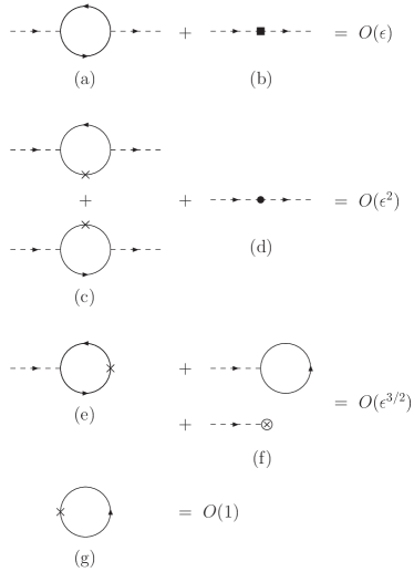
Figure 3: Four apparent exceptions of the naive power counting rule of $\epsilon$ [(a), (c), (e), (g)]. The boson self-energy diagram (a) or (c) is combined with the vertex from $\mathcal{L}_{2}$, (b) or (d), to restore the naive $\epsilon$ power counting. The tadpole diagram in (e) cancels with other tadpole diagrams at the minimum of the effective potential. The vacuum diagram (g) is the only exception of the naive power counting rule of $\epsilon$, which is $O(1)$ instead of $O(\epsilon)$.

Similarly, the diagram in Fig. 3(c) representing the boson self-energy with one $\mu$ insertion gives

$$-i \Pi_{\mathrm{c}}(p)=2\mu\,g^{2}\int\!\frac{dk}{(2\pi)^{d+1}}$$ (39)

$$\qquad\times\left[G_{11}\!\left(k+\frac{p}{2}\right)^{2}-G_{12}\!\left(k+\frac{p}{2}\right)^{2}\right]G_{22}\!\left(k-\frac{p}{2}\right),$$

which also contains a $1/\epsilon$ singularity, and hence is $O(\epsilon)$ instead of the naive $O(\epsilon^{2})$. The leading part of this diagram is

$$\Pi_{\mathrm{c}}(p)=-2\mu\,g^{2}\int_{\bm{k}}\frac{1}{4\varepsilon_{\bm{k}}^{\,2}}+\cdots=-2\mu+O(\epsilon^{2}),$$ (40)

which is canceled out exactly by adding the second vertex from $\mathcal{L}_{2}$. Then the sum of Figs. 3(c) and 3(d) is again $O(\epsilon^{2})$, consistent with the naive power counting.

The $\varphi$ tadpole diagram with one $\mu$ insertion in Fig. 3(e) is

$$\begin{split}\Xi_{\mathrm{e}}&=-\mu g\int\!\frac{dk}{(2\pi)^{d+1}}\left[G_{11}(k)-G_{22}(k)\right]G_{21}(k)\\ &=ig\mu\phi_{0}\int_{\bm{k}}\frac{\varepsilon_{\bm{k}}}{2E_{\bm{k}}^{\,3}}=\frac{ig\mu}{\epsilon\phi_{0}}\left(\frac{m\phi_{0}}{2\pi}\right)^{2}+O(\epsilon^{3/2}),\end{split}$$ (41)

which is $O(\epsilon^{1/2})$ instead of the naive $O(\epsilon^{3/2})$. This tadpole diagram should be canceled by other tadpole diagrams of order $O(\epsilon^{1/2})$ in Fig. 3(f),

$$\begin{split}\Xi_{\mathrm{f}}&=g\int\!\frac{dk}{(2\pi)^{d+1}}G_{21}(k)-i\frac{g\phi_{0}}{c_{0}}\\ &=-\frac{ig}{2}\left(\frac{m\phi_{0}}{2\pi}\right)^{2}-i\frac{g\phi_{0}}{c_{0}}+O(\epsilon^{3/2}).\end{split}$$ (42)

The condition of cancellation, $\Xi_{\mathrm{e}}+\Xi_{\mathrm{f}}=0$, gives the gap equation that determines $\phi_{0}(\mu)$ to the leading order in $\epsilon$. The solution to the gap equation is

$$\phi_{0}=\frac{2\mu}{\epsilon}-\frac{2}{c_{0}}\left(\frac{2\pi}{m}\right)^{2}+O(\epsilon).$$ (43)

When $c_{0}<0$, this solution can be written in terms of the binding energy $\varepsilon_{\mathrm{b}}$ as $\phi_{0}=(2\mu+\varepsilon_{\mathrm{b}})/\epsilon$. The previously made assumption $\mu/\phi_{0}=O(\epsilon)$ is indeed correct. As we will see later, the cancellation of the tadpole diagrams is automatically achieved by the minimization of the effective potential.

Finally, the one-loop vacuum diagram with one $\mu$ insertion in Fig. 3(g) also contains the $1/\epsilon$ singularity as

$$\begin{split}&i\mu\int\!\frac{dk}{(2\pi)^{d+1}}\left[G_{11}(k)-G_{22}(k)\right]\\ &\ =\mu\int_{\bm{k}}\frac{\varepsilon_{\bm{k}}}{E_{\bm{k}}}=-\frac{\mu}{\epsilon}\left(\frac{m\phi_{0}}{2\pi}\right)^{2}+O(\epsilon).\end{split}$$ (44)

The leading part of this diagram is $O(1)$ instead of naive $O(\epsilon)$ and cannot be canceled by any other diagrams. Therefore, Fig. 3(g) $\sim O(1)$ is the only exception of our naive power counting rule of $\epsilon$.

Thus, we can now develop a diagrammatic technique for the Fermi gas near the unitarity limit where $g^{2}/|c_{0}|\sim\mu$ in terms of the systematic expansion over $\epsilon=4-d$. The power counting rule of $\epsilon$ is summarized as follows:

1. We consider $\mu/\phi_{0}\sim\epsilon$ and regard $\phi_{0}$ as $O(1)$.

2. For any Green’s function, we write down all Feynman diagrams according to the Feynman rules in Fig. 2 using the propagators from $\mathcal{L}_{0}$ and the vertices from $\mathcal{L}_{1}$.

3. If there is any subdiagram of the type in Fig. 3(a) or 3(c), we add the same Feynman diagram where the subdiagram is replaced by the vertex from $\mathcal{L}_{2}$, Fig. 3(b) or 3(d).

4. The power of $\epsilon$ for the given Feynman diagram will be $O(\epsilon^{N_{g}/2+N_{\mu}})$, where $N_{g}$ is the number of couplings $g$ and $N_{\mu}$ is the number of chemical potential insertions.

5. The only exception is the diagram in Fig. 3(g) which is $O(1)$.

We note that the sum of all tadpole diagrams in Figs. 3(e) and 3(f) vanishes if $\phi_{0}$ is the solution of the gap equation.

III.3 Effective potential to leading and next-to-leading orders

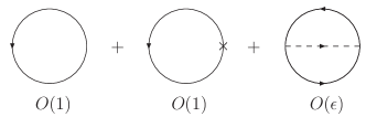
Figure 4: Vacuum diagrams contributing to the effective potential up to the next-to-leading order in $\epsilon$. The second diagram is $O(1)$ instead of naive $O(\epsilon)$ because of the $1/\epsilon$ singularity.

We now perform calculations to the leading and next-to-leading orders in $\epsilon$, employing the Feynman rules and the $\epsilon$ power counting that have just been developed. To find the dependence of $\phi_{0}$ on $\mu$, we use the effective potential method Peskin:1995ev in which this dependence follows from the minimization of the effective potential $V_{\mathrm{eff}}(\phi_{0})$. The effective potential at the tree level is given by

$$V_{0}(\phi_{0})=\frac{\phi_{0}^{\,2}}{c_{0}}.$$ (45)

Up to the next-to-leading order, the effective potential receives contributions from three vacuum diagrams drawn in Fig. 4: fermion loops with and without a $\mu$ insertion and a fermion loop with one boson exchange.

The contribution from two one-loop diagrams is $O(1)$ and given by

$$\begin{split}V_{1}(\phi_{0})&=i\int\!\frac{dp}{(2\pi)^{d+1}}\mathop{\mathrm{Tr}}\left[\ln G^{-1}(p)+\mu\sigma_{3}G(p)\right]\\ &=-\int_{\bm{p}}\left(E_{\bm{p}}-\mu\frac{\varepsilon_{\bm{p}}}{E_{\bm{p}}}\right).\end{split}$$ (46)

Using the formula in Eq. (10), we can perform the integration over ${\bm{p}}$ to find

$$V_{1}(\phi_{0})=$$ (47)

$$-\frac{\left(\frac{m\phi_{0}}{2\pi}\right)^{\frac{d}{2}}}{2\Gamma(\frac{d}{2})}\left[\frac{\Gamma(\frac{d}{4})\Gamma(-\frac{1}{2}-\frac{d}{4})}{\Gamma(-\frac{1}{2})}\phi_{0}-\frac{\Gamma(\frac{d}{4}+\frac{1}{2})\Gamma(-\frac{d}{4})}{\Gamma(\frac{1}{2})}\mu\right].$$

Substituting $d=4-\epsilon$ and expanding in terms of $\epsilon$ up to $O(\epsilon)$, this contribution becomes

$$V_{1}(\phi_{0}) =\frac{\phi_{0}}{3}\left[1+\frac{7-3(\gamma+\ln 2)}{6}\epsilon\right]\left(\frac{m\phi_{0}}{2\pi}\right)^{d/2}$$ (48)

$$-\frac{\mu}{\epsilon}\left[1+\frac{1-2(\gamma-\ln 2)}{4}\epsilon\right]\left(\frac{m\phi_{0}}{2\pi}\right)^{d/2}\!+O(\epsilon^{2}),$$

where $\gamma\approx 0.57722$ is the Euler-Mascheroni constant.

The contribution of the two-loop diagram is $O(\epsilon)$ and given by

$$V_{2}(\phi_{0}) =g^{2}\int\!\frac{dp\,dq}{(2\pi)^{2d+2}}\mathop{\mathrm{Tr}}\left[G(p)\sigma_{+}G(q)\sigma_{-}\right]D(p-q)$$

$$=g^{2}\int\!\frac{dp\,dq}{(2\pi)^{2d+2}}\,G_{11}(p)G_{22}(q)D(p-q).$$ (49)

Performing the integrations over $p_{0}$ and $q_{0}$, we obtain

$$V_{2}(\phi_{0})=-\frac{g^{2}}{4}\!\int_{{\bm{p}}{\bm{q}}}\frac{(E_{\bm{p}}-\varepsilon_{\bm{p}})(E_{\bm{q}}-\varepsilon_{\bm{q}})}{E_{\bm{p}}E_{\bm{q}}(E_{\bm{p}}+E_{\bm{q}}+\varepsilon_{{\bm{p}}-{\bm{q}}}/2)}.$$ (50)

Since this is a next-to-leading-order diagram and the integrals converge at $d=4$, we can evaluate the integrations at $d=4$. Changing the integration variables to $x=\varepsilon_{\bm{p}}/\phi_{0}$, $y=\varepsilon_{\bm{q}}/\phi_{0}$, and $\cos\theta=\hat{\bm{p}}\cdot\hat{\bm{q}}$, the integral can be transformed into

$$V_{2}(\phi_{0}) =-\epsilon\left(\frac{m\phi_{0}}{2\pi}\right)^{d/2}\frac{\phi_{0}}{\pi}\int_{0}^{\infty}\!dx\int_{0}^{\infty}\!dy\int_{0}^{\pi}\!d\theta$$ (51)

$$\qquad\times xy\sin^{2}\theta\,\frac{[f(x)-x][f(y)-y]}{f(x)f(y)\left[g(x,y)-\sqrt{xy}\cos\theta\right]},$$

with $f(x)=\sqrt{x^{2}+1}$ and $g(x,y)=f(x)+f(y)+\frac{1}{2}(x+y)$. The integration over $\theta$ can be performed analytically to lead to

$$V_{2}(\phi_{0})=-C\epsilon\left(\frac{m\phi_{0}}{2\pi}\right)^{d/2}\phi_{0},$$ (52)

where the constant $C$ is given by a two-dimensional integral

$$\begin{split}C&=\int_{0}^{\infty}\!dx\int_{0}^{\infty}\!dy\,\frac{[f(x)-x][f(y)-y]}{f(x)f(y)}\\ &\qquad\qquad\qquad\times\left[g(x,y)-\sqrt{g^{2}(x,y)-xy}\right].\end{split}$$ (53)

A numerical integration over $x$ and $y$ gives

$$C\approx 0.14424.$$ (54)

Now, gathering up Eqs. (45), (48), and (51), we obtain the effective potential up to the next-to-leading order in $\epsilon$,

$$\begin{split}V_{\mathrm{eff}}(\phi_{0})&=V_{0}(\phi_{0})+V_{1}(\phi_{0})+V_{2}(\phi_{0})\\ &=\frac{\phi_{0}^{\,2}}{c_{0}}+\left[\frac{\phi_{0}}{3}\left\{1+\frac{7-3(\gamma+\ln 2)}{6}\epsilon-3C\epsilon\right\}-\frac{\mu}{\epsilon}\left\{1+\frac{1-2(\gamma-\ln 2)}{4}\epsilon\right\}\right]\left(\frac{m\phi_{0}}{2\pi}\right)^{d/2}\!+O(\epsilon^{2}).\end{split}$$ (55)

The condition that $\phi_{0}$ minimizes the effective potential gives the gap equation; $\partial V_{\mathrm{eff}}/\partial\phi_{0}=0$. The solution to this equation is

$$\phi_{0} =\frac{2\mu}{\epsilon}\left[1+\left(3C-1+\ln 2\right)\epsilon\right]$$ (56)

$$\quad-\frac{2\phi_{0}^{\,\epsilon/2}}{c_{0}}\left(\frac{2\pi}{m}\right)^{d/2}\left[1+\left(3C-1+\frac{\gamma+\ln 2}{2}\right)\epsilon\right].$$

Using the relation of $c_{0}$ with the binding energy of boson $\varepsilon_{\mathrm{b}}$ in Eq. (20), we can rewrite the solution of the gap equation in terms of $\varepsilon_{\mathrm{b}}$ up to the next-to-leading order in $\epsilon$ as

$$\phi_{0} =\frac{2\mu}{\epsilon}\left[1+\left(3C-1+\ln 2\right)\epsilon\right]$$ (57)

$$\quad+\frac{\varepsilon_{\mathrm{b}}}{\epsilon}\left[1+\left(3C-\frac{1}{2}+\ln 2-\frac{1}{2}\ln\frac{\varepsilon_{\mathrm{b}}}{\phi_{0}}\right)\epsilon\right].$$

We note that the leading term in Eq. (57) could be reproduced using the mean field approximation, but the $O(\epsilon)$ corrections are not. The $O(\epsilon)$ correction proportional to the constant $C$ is a result of the summation of fluctuations around the classical solution and is beyond the mean field approximation.

III.4 Thermodynamic quantities near unitarity

The value of the effective potential $V_{\mathrm{eff}}$ at its minimum determines the pressure $P=-V_{\mathrm{eff}}(\phi_{0})$ at a given chemical potential $\mu$ and a given binding energy of boson $\varepsilon_{\mathrm{b}}$. Substituting the dependence of $\phi_{0}$ on $\mu$ and $\varepsilon_{\mathrm{b}}$ in Eq. (57), we obtain the pressure as

$$P=\frac{\phi_{0}}{6}\left[1+\left(\frac{17}{12}{-}3C{-}\frac{\gamma{+}\ln 2}{2}\right)\epsilon-\frac{3\varepsilon_{\mathrm{b}}}{4\phi_{0}}\right]\left(\frac{m\phi_{0}}{2\pi}\right)^{d/2}.$$ (58)

The fermion number density $N$ is determined by differentiating the pressure in terms of $\mu$ as

$$N=\frac{\partial P}{\partial\mu}=\frac{1}{\epsilon}\left[1+\frac{1-2\gamma+2\ln 2}{4}\epsilon\right]\left(\frac{m\phi_{0}}{2\pi}\right)^{d/2}.$$ (59)

Then the Fermi energy of a $d$-dimensional free gas with the same number density is

$$\varepsilon_{\mathrm{F}}=\frac{2\pi}{m}\left[\frac{1}{2}\Gamma\left(\frac{d}{2}+1\right)N\right]^{2/d}=\frac{\phi_{0}}{\epsilon^{2/d}}\left(1-\frac{1-\ln 2}{4}\epsilon\right).$$ (60)

The nontrivial power of $\epsilon$ appears because we have raised $N\sim\epsilon^{-1}$ to the power of $2/d$.

From Eqs. (57) and (60), we can determine the ratio of the chemical potential and the Fermi energy $\mu/\varepsilon_{\mathrm{F}}$ near the unitary limit as

$$\frac{\mu}{\varepsilon_{\mathrm{F}}} =\frac{\epsilon^{3/2}}{2}\exp\!\left(\frac{\epsilon\ln\epsilon}{8-2\epsilon}\right)\left[1-\left(3C-\frac{5}{4}(1-\ln 2)\right)\epsilon\right]$$

$$\qquad-\frac{\varepsilon_{\mathrm{b}}}{2\varepsilon_{\mathrm{F}}}\left[1+\frac{\epsilon}{2}+\frac{\epsilon\ln\epsilon}{4}-\frac{\epsilon}{2}\ln\frac{\varepsilon_{\mathrm{b}}}{\varepsilon_{\mathrm{F}}}\right].$$ (61)

The $\ln\epsilon$ term in the second line originates from the substitution of $\phi_{0}=\epsilon^{1/2}\varepsilon_{\mathrm{F}}$ into the $\ln\varepsilon_{\mathrm{b}}/\phi_{0}$ term in Eq. (57). We note again that if one is interested in the extrapolation to $d=3$, one can use Eq. (22) to relate $\varepsilon_{\mathrm{b}}/\varepsilon_{\mathrm{F}}$ to $ak_{\mathrm{F}}$. The first term in Eq. (III.4) gives the universal parameter of the unitary Fermi gas $\xi\equiv\left.\mu/\varepsilon_{\mathrm{F}}\right|_{\varepsilon_{\mathrm{b}}=0}$,

$$\begin{split}\xi&=\frac{\epsilon^{3/2}}{2}\left[1+\frac{\epsilon\ln\epsilon}{8}-\left(3C-\frac{5}{4}(1-\ln 2)\right)\epsilon\right]\\ &=\frac{1}{2}\epsilon^{3/2}+\frac{1}{16}\epsilon^{5/2}\ln\epsilon-0.0246\,\epsilon^{5/2}+\cdots.\end{split}$$ (62)

Here we have used the numerical value for $C\approx 0.14424$ in Eq. (54). The smallness of the coefficient in front of $\epsilon^{5/2}$ is a result of a cancellation between the two-loop correction and the subleading terms from the expansion of the one-loop diagrams around $d=4$.

Using Eqs. (58), (59), and (60), the pressure near the unitarity limit normalized by $\varepsilon_{\mathrm{F}}N$ is given by

$$\frac{P}{\varepsilon_{\mathrm{F}}N}=\frac{2}{d+2}\xi-\frac{\varepsilon_{\mathrm{b}}}{8\varepsilon_{\mathrm{F}}}\epsilon.$$ (63)

Then the energy density $E=\mu N-P$ can be calculated from Eqs. (III.4) and (63) as

$$\frac{E}{\varepsilon_{\mathrm{F}}N}=\frac{d}{d+2}\xi-\frac{\varepsilon_{\mathrm{b}}}{2\varepsilon_{\mathrm{F}}}\left[1+\frac{\epsilon}{4}+\frac{\epsilon\ln\epsilon}{4}-\frac{\epsilon}{2}\ln\frac{\varepsilon_{\mathrm{b}}}{\varepsilon_{\mathrm{F}}}\right].$$ (64)

The pressure and energy density in the unitarity limit are obtained from $\xi$ via the universal relations depending only on the dimensionality of space.

III.5 Quasiparticle spectrum

The $\epsilon$ expansion we have developed is also useful for the calculations of physical observables other than the thermodynamic quantities. Here we shall look at the dispersion relation of fermion quasiparticles. To the leading order in $\epsilon$, the dispersion relation is given by $\omega_{\mathrm{F}}({\bm{p}})=E_{\bm{p}}=\sqrt{\varepsilon_{\bm{p}}^{\,2}+\phi_{0}^{\,2}}$, which has a minimum at zero momentum ${\bm{p}}=\bm{0}$ with the energy gap equal to $\Delta=\phi_{0}=(2\mu+\varepsilon_{\mathrm{b}})/\epsilon$. The next-to-leading-order corrections to the dispersion relation come from three sources: from the correction of $\phi_{0}$ in Eq. (57), from a $\mu$ insertion to the fermion propagator, and from the one-loop self-energy diagrams $-i\Sigma(p)$ depicted in Fig. 5.

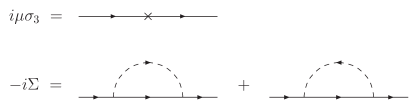
Figure 5: Corrections to the fermion self-energy of order $O(\epsilon)$; a $\mu$ insertion and one-loop diagrams.

Using the Feynman rules, the one-loop diagram of the fermion self-energy in Fig. 5 is given by

$$\begin{split}-i\Sigma(p)=g^{2}\int\!\frac{dk}{(2\pi)^{d+1}}\,&\left[\sigma_{+}G(k)\sigma_{-}D(p-k)\right.\\ &\left.+\sigma_{-}G(k)\sigma_{+}D(k-p)\right].\end{split}$$ (65)

There are corrections only to the diagonal elements of the self-energy and each element is evaluated as

$$\begin{split}\Sigma_{11}(p)&=ig^{2}\int\!\frac{dk}{(2\pi)^{d+1}}\,G_{22}(k)D(p-k)\\ &=-\frac{g^{2}}{2}\int_{\bm{k}}\frac{E_{\bm{k}}-\varepsilon_{\bm{k}}}{E_{\bm{k}}(E_{\bm{k}}+\varepsilon_{{\bm{k}}-{\bm{p}}}/2-p_{0}-i\delta)},\end{split}$$ (66)

and

$$\begin{split}\Sigma_{22}(p)&=ig^{2}\int\!\frac{dk}{(2\pi)^{d+1}}\,G_{11}(k)D(k-p)\\ &=\frac{g^{2}}{2}\int_{\bm{k}}\frac{E_{\bm{k}}-\varepsilon_{\bm{k}}}{E_{\bm{k}}(E_{\bm{k}}+\varepsilon_{{\bm{k}}-{\bm{p}}}/2+p_{0}-i\delta)}.\end{split}$$ (67)

The dispersion relation of the fermion quasiparticle $\omega_{\mathrm{F}}({\bm{p}})$ is obtained as a pole of the fermion propagator $\det[G^{-1}(\omega,{\bm{p}})+\mu\sigma_{3}-\Sigma(\omega,{\bm{p}})]=0$, which reduces to the following equation:

$$\begin{vmatrix}\omega-\varepsilon_{\bm{p}}+\mu-\Sigma_{11}(\omega,{\bm{p}})&\phi_{0}\\ \phi_{0}&\omega+\varepsilon_{\bm{p}}-\mu-\Sigma_{22}(\omega,{\bm{p}})\end{vmatrix}=0.$$ (68)

To find the $O(\epsilon)$ correction to the dispersion relation, we only have to evaluate the self-energy $\Sigma(\omega,{\bm{p}})$ with $\omega$ given by the leading order solution $\omega=E_{\bm{p}}$. Denoting $\Sigma_{11}(E_{\bm{p}},{\bm{p}})$ and $\Sigma_{22}(E_{\bm{p}},{\bm{p}})$ simply by $\Sigma_{11}$ and $\Sigma_{22}$ and solving Eq. (68) in terms of $\omega$, we obtain the dispersion relation of the fermion quasiparticle as

$$\omega_{\mathrm{F}}({\bm{p}})=E_{\bm{p}}+\frac{\Sigma_{11}+\Sigma_{22}}{2}+\frac{\Sigma_{11}-\Sigma_{22}-2\mu}{2E_{\bm{p}}}\varepsilon_{\bm{p}}+O(\epsilon^{2}).$$ (69)

In order to find the energy gap of the fermion quasiparticle, since the minimum of the dispersion relation will appear at small momentum $\varepsilon_{\bm{p}}\sim\mu$, we can expand $\Sigma(E_{\bm{p}},{\bm{p}})$ around zero momentum ${\bm{p}}=0$ as $\Sigma(E_{\bm{p}},{\bm{p}})=\Sigma^{0}(\phi_{0},\bm{0})+\Sigma^{\prime}(\phi_{0},\bm{0})\,\varepsilon_{\bm{p}}/\phi_{0}$. Performing the integration over ${\bm{k}}$ in $\Sigma$ analytically, we have

$$\begin{split}\Sigma_{11}(\phi_{0},{\bm{p}})&=\epsilon\left(2-8\ln 3+8\ln 2\right)\phi_{0}\\ &\qquad+\epsilon\left(-\frac{8}{3}+8\ln 3-8\ln 2\right)\varepsilon_{\bm{p}},\end{split}$$ (70)

and

$$\begin{split}\Sigma_{22}(\phi_{0},{\bm{p}})&=\epsilon\left(-2-8\ln 3+16\ln 2\right)\phi_{0}\\ &\qquad+\epsilon\left(-\frac{7}{3}-8\ln 3+16\ln 2\right)\varepsilon_{\bm{p}}.\end{split}$$ (71)

Introducing these expressions into Eq. (69), we find the fermion dispersion relation around its minimum has the following form:

$$\omega_{\mathrm{F}}({\bm{p}})\simeq\Delta+\frac{(\varepsilon_{\bm{p}}-\varepsilon_{0})^{2}}{2\phi_{0}}\simeq\sqrt{(\varepsilon_{\bm{p}}-\varepsilon_{0})^{2}+\Delta^{2}}.$$ (72)

Figure 6: Illustration of the dispersion relation of the fermion quasiparticle in the unitarity limit from the $\epsilon$ expansion. $\omega_{\mathrm{F}}({\bm{p}})=\sqrt{(\varepsilon_{\bm{p}}-\varepsilon_{0})^{2}+\Delta^{2}}$ in Eq. (72) is plotted as a function of $\varepsilon_{\bm{p}}={\bm{p}}^{2}/2m$. Values on both axes are extrapolated results to $\epsilon=1$ in units of the chemical potential $\mu$.

Here $\Delta$ is the energy gap of the fermion quasiparticle, which is given by

$$\begin{split}\Delta&=\phi_{0}+\frac{\Sigma_{11}^{0}+\Sigma_{22}^{0}}{2}\\ &=\left[1-\left(8\ln 3-12\ln 2\right)\epsilon+O(\epsilon^{2})\right]\phi_{0}.\end{split}$$ (73)

The minimum of the dispersion curve is located at a nonzero value of momentum, $|{\bm{p}}|=(2m\varepsilon_{0})^{1/2}$, where

$$\begin{split}\varepsilon_{0}&=\mu+\frac{\Sigma_{22}^{0}-\Sigma_{11}^{0}}{2}-\frac{\Sigma_{11}^{\prime}+\Sigma_{22}^{\prime}}{2}\\ &=\mu+\frac{\epsilon\phi_{0}}{2}+O(\epsilon^{2}).\end{split}$$ (74)

Then, introducing the solution of the gap equation (57), the energy gap $\Delta$ as a function of the chemical potential and the binding energy is given by

$$\Delta =\frac{2\mu}{\epsilon}\left[1+(3C-1-8\ln 3+13\ln 2)\epsilon\right]$$

$$\quad+\frac{\varepsilon_{\mathrm{b}}}{\epsilon}\left[1+\left(3C-\frac{1}{2}-8\ln 3+13\ln 2-\frac{1}{2}\ln\frac{\varepsilon_{\mathrm{b}}}{\Delta}\right)\epsilon\right]$$

$$=\frac{2\mu}{\epsilon}\left(1-0.345\,\epsilon\right)$$ (75)

$$\quad+\frac{\varepsilon_{\mathrm{b}}}{\epsilon}\left[1+0.155\,\epsilon-\frac{\epsilon\ln\epsilon}{2}+\frac{\epsilon}{2}\ln\!\left(1+\frac{2\mu}{\varepsilon_{\mathrm{b}}}\right)\right],$$

while $\varepsilon_{0}$ is given by

$$\varepsilon_{0}=2\mu+\frac{\varepsilon_{\mathrm{b}}}{2}.$$ (76)

Note the difference with the mean field approximation, in which $\varepsilon_{0}=\mu$.

When $\varepsilon_{0}$ is positive, the fermion dispersion curve has its minimum at nonzero value of momentum as in the BCS limit, while the minimum is located at zero momentum when $\varepsilon_{0}$ is negative as in the BEC limit. We find the former $(\varepsilon_{0}=2\mu>0)$ is the case in the unitarity limit. The dispersion curve of the fermion quasiparticle $\omega_{\mathrm{F}}({\bm{p}})$ in the unitarity limit $\varepsilon_{\mathrm{b}}=0$ is illustrated in Fig 6. In particular, the difference between the fermion quasiparticle energy at zero momentum and at its minimum is given by $\varepsilon_{0}^{\,2}/2\phi_{0}=\epsilon\mu\sim O(\epsilon^{2})$.

III.6 Location of the splitting point

Let us consider the situation where the binding energy $\varepsilon_{\mathrm{b}}$ is increasing from zero while the number density $N$ is kept fixed. Then $\Delta>0$ is held fixed but $\mu$ is changing. Since to the leading order in $\epsilon$, the chemical potential as a function of the energy gap is given by $2\mu=\epsilon\Delta-\varepsilon_{\mathrm{b}}$, the location of the minimum of the dispersion curve can be written as

$$\varepsilon_{0}=\epsilon\Delta-\frac{\varepsilon_{\mathrm{b}}}{2}.$$ (77)

Therefore, $\varepsilon_{0}$ decreases as $\varepsilon_{\mathrm{b}}$ increases. When the binding energy reaches $\varepsilon_{\mathrm{b}}=2\epsilon\Delta$, the minimum of the dispersion curve sits exactly at zero momentum ${\bm{p}}=\bm{0}$. This point is referred to as a splitting point son05 . We find the splitting point is located on the BEC side of the unitarity limit where the binding energy is positive $\varepsilon_{\mathrm{b}}=2\epsilon\Delta>0$ and the chemical potential is negative $2\mu=-\epsilon\Delta$. This splitting point will play an important role to determine the phase structure of the polarized Fermi gas in the unitary regime as we will study in Sec. IV.

III.7 Extrapolation to $\epsilon=1$

Finally, we discuss the extrapolation of the series expansion to the physical case in three spatial dimensions. Although the formalism is based on the smallness of $\epsilon$, we see that the next-to-leading-order corrections are reasonably small compared to the leading terms even at $\epsilon=1$. If we naively use only the leading and next-to-leading-order results for $\xi$ in Eq. (62), $\Delta$ in Eq. (III.5), and $\varepsilon_{0}$ in Eq. (76) in the unitarity limit, their extrapolations to $\epsilon=1$ give for three spatial dimensions

$$\xi\approx 0.475,\qquad\frac{\Delta}{\mu}\approx 1.31,\qquad\frac{\varepsilon_{0}}{\mu}\approx 2.$$ (78)

They are reasonably close to the results of recent Monte Carlo simulations, which yield $\xi\approx 0.42$, $\Delta/\mu\approx 1.2$, and $\varepsilon_{0}/\mu\approx 1.9$ Carlson:2005kg . They are also consistent with recent experimental measurements of $\xi$, where $\xi=0.51\pm 0.04$ Thomas05 and $\xi=0.46\pm 0.05$ Hulet-polarized . These agreements can be taken as a strong indication that the $\epsilon$ expansion is useful even at $\epsilon=1$.

Our $\epsilon$ expansion predicts the behavior of the thermodynamic quantities near the unitarity limit. From Eqs. (63), (64), and (III.4), the extrapolations to the three spatial dimensions $\epsilon=1$ lead to

$$\frac{P}{\varepsilon_{\mathrm{F}}N} \approx\frac{2}{d+2}\,\xi-\frac{1}{8}\frac{\varepsilon_{\mathrm{b}}}{\varepsilon_{\mathrm{F}}},$$ (79)

$$\frac{E}{\varepsilon_{\mathrm{F}}N} \approx\frac{d}{d+2}\,\xi-\frac{1}{4}\frac{\varepsilon_{\mathrm{b}}}{\varepsilon_{\mathrm{F}}}\left(\frac{5}{2}-\ln\frac{\varepsilon_{\mathrm{b}}}{\varepsilon_{\mathrm{F}}}\right),\phantom{\frac{\frac{\int}{\int}}{\frac{\int}{\int}}}$$ (80)

$$\frac{\mu}{\varepsilon_{\mathrm{F}}} \approx\xi-\frac{1}{4}\frac{\varepsilon_{\mathrm{b}}}{\varepsilon_{\mathrm{F}}}\left(3-\ln\frac{\varepsilon_{\mathrm{b}}}{\varepsilon_{\mathrm{F}}}\right).$$ (81)

The pressure, energy density, and chemical potential at fixed density are decreasing functions of the binding energy $\varepsilon_{\mathrm{b}}$ with the slope shown above. In Sec. VI, we will make a discussion to improve the extrapolation of the series expansion by imposing the exact result at $d=2$ as a boundary condition.

We can also try to determine the location of the splitting point. At this point, the deviation from the unitarity point measured by the binding energy per Fermi energy is given by

$$\frac{\varepsilon_{\mathrm{b}}}{\varepsilon_{\mathrm{F}}}=\frac{2}{\epsilon^{2/d-1}}[1+O(\epsilon)]\approx 2\qquad\text{at}\ \ d=3.$$ (82)

Comparing with Eq. (22), one finds $ak_{\mathrm{F}}\approx 1$ at the splitting point. Since this result is known only to the leading order in $\epsilon$, one must be cautious with the numerical value. However, certain qualitative features are probably correct: the splitting point is located on the BEC side of the unitarity limit ($a>0$) and the chemical potential $\mu/\varepsilon_{\mathrm{F}}\approx-0.5$ is negative at this point.

IV Phase structure of polarized Fermi gas

IV.1 Effective potential at finite superfluid velocity

Here we apply the $\epsilon$ expansion developed in the previous section to the unitary Fermi gas with unequal densities for the two fermion components. We put special emphasis on investigating the phase structure of polarized Fermi gas in the unitary regime, which has a direct relation with the recent measurements in atomic traps Ketterle-polarized ; Hulet-polarized ; Ketterle-polarized2 ; Ketterle-polarized3 . For this purpose, we generalize our formalism to take into account the possibility of a spatially varying condensate where $\langle\phi(x)\rangle=e^{2im\bm{v}_{\mathrm{s}}\cdot\bm{x}}\phi_{0}$ with $\bm{v}_{\mathrm{s}}$ being the superfluid velocity. The factor $e^{2im\bm{v}_{\mathrm{s}}\cdot\bm{x}}$ in front of $\phi_{0}$ in the Lagrangian density can be absorbed by making the Galilean transformation on the fermion field as $\psi_{\sigma}(x)\to e^{im\bm{v}_{\mathrm{s}}\cdot\bm{x}}\psi_{\sigma}(x)$ and the boson field as $\varphi(x)\to e^{2im\bm{v}_{\mathrm{s}}\cdot\bm{x}}\varphi(x)$. Accordingly, the fermion propagator in Eq. (29) is modified as

$$\begin{split}G(p_{0},{\bm{p}})&=\frac{1}{(p_{0}+H-{\bm{p}}\cdot\bm{v}_{\mathrm{s}})^{2}-(\varepsilon_{\bm{p}}+\varepsilon_{m\bm{v}_{\mathrm{s}}})^{2}-\phi_{0}^{\,2}+i\delta}\\ &\quad\times\begin{pmatrix}p_{0}+H+\varepsilon_{{\bm{p}}-m\bm{v}_{\mathrm{s}}}&-\phi_{0}\\ -\phi_{0}&p_{0}+H-\varepsilon_{{\bm{p}}+m\bm{v}_{\mathrm{s}}}\end{pmatrix},\end{split}$$ (83)

while the boson propagator in Eq. (30) is modified as

$$D(p_{0},{\bm{p}})=\left(p_{0}-\frac{\varepsilon_{{\bm{p}}+2m\bm{v}_{\mathrm{s}}}}{2}+i\delta\right)^{-1}.$$ (84)

The value of the superfluid velocity $\bm{v}_{\mathrm{s}}$ is determined by minimizing the $\bm{v}_{\mathrm{s}}$ dependent part of the effective potential $V_{H}(\bm{v}_{\mathrm{s}})$. As far as the polarization $H$ is sufficiently small compared to the energy gap $\Delta$ of the fermion quasiparticle, $V_{H}(\bm{v}_{\mathrm{s}})$ to the leading order in $\epsilon$ is given by the fermion one-loop diagram with the propagator in Eq. (83) as follows:

$$V_{H<\Delta}(\bm{v}_{\mathrm{s}})=-\int_{\bm{p}}\sqrt{\left(\varepsilon_{\bm{p}}+\varepsilon_{m\bm{v}_{\mathrm{s}}}\right)^{2}+\phi_{0}^{\,2}}.$$ (85)

Since it will turn out that $\varepsilon_{m\bm{v}_{\mathrm{s}}}$ is $O(\epsilon^{11})$, we can expand the integrand in terms of $\varepsilon_{m\bm{v}_{\mathrm{s}}}/\phi_{0}$ to lead to

$$V_{H<\Delta}(\bm{v}_{\mathrm{s}})=-\varepsilon_{m\bm{v}_{\mathrm{s}}}\int_{\bm{p}}\frac{\varepsilon_{\bm{p}}}{E_{\bm{p}}}\simeq\frac{\varepsilon_{m\bm{v}_{\mathrm{s}}}}{\epsilon}\left(\frac{m\phi_{0}}{2\pi}\right)^{2}.$$ (86)

Using the result on the fermion number density $N$ in Eq. (59), this part can be rewritten as $V_{H<\Delta}(\bm{v}_{\mathrm{s}})=N\varepsilon_{m\bm{v}_{\mathrm{s}}}$, which represents the energy cost due to the presence of the superfluid flow.

If $H-{\bm{p}}\cdot\bm{v}_{\mathrm{s}}$ reaches the bottom of the fermion quasiparticle spectrum $\Delta+(\varepsilon_{\bm{p}}+\varepsilon_{m\bm{v}_{\mathrm{s}}}-\varepsilon_{0})^{2}/2\phi_{0}$, $V_{H}(\bm{v}_{\mathrm{s}})$ receives an additional contribution from the filled fermion quasiparticles. Since $\varepsilon_{m\bm{v}_{\mathrm{s}}}\sim\epsilon^{11}$ is small, we can neglect it in the quasiparticle energy. Then the $\bm{v}_{\mathrm{s}}$ dependent part of the effective potential is given by

$$V_{H}(\bm{v}_{\mathrm{s}})=N\varepsilon_{m\bm{v}_{\mathrm{s}}}-\int_{\bm{p}}\left[H-{\bm{p}}\cdot\bm{v}_{\mathrm{s}}-\omega_{\mathrm{F}}({\bm{p}})\right]_{>},$$ (87)

where we have introduced a notation $(x)^{y}_{>}=x^{y}\,\theta(x)$ and $\omega_{\mathrm{F}}({\bm{p}})$ is the fermion quasiparticle spectrum $\omega_{\mathrm{F}}({\bm{p}})=\Delta+(\varepsilon_{\bm{p}}-\varepsilon_{0})^{2}/2\phi_{0}$ derived in Eq. (72). The effective potential $V_{H}(\bm{v}_{\mathrm{s}})$ to the leading order in $\epsilon$ has the same form as that studied based on the effective field theory in son05 .

IV.2 Critical polarizations

Now we evaluate the effective potential $V_{H}(\bm{v}_{\mathrm{s}})$ at $d=4$ as a function of $\bm{v}_{\mathrm{s}}$ and $H$. Changing the integration variables to $z=\varepsilon_{\bm{p}}/\phi_{0}$ and $w=\hat{\bm{p}}\cdot\hat{\bm{v}}_{\mathrm{s}}$, we have

$$\begin{split}V_{H}(\bm{v}_{\mathrm{s}})&=\left(\frac{m\phi_{0}}{2\pi}\right)^{2}\left[\frac{\varepsilon_{m\bm{v}_{\mathrm{s}}}}{\epsilon}-\frac{2}{\pi}\int_{0}^{\infty}\!dz\!\int_{-1}^{1}\!dw\,z\sqrt{1-w^{2}}\right.\\ &\left.\times\left(H-\Delta-\frac{(z-z_{0})^{2}}{2}\phi_{0}-2\sqrt{z\phi_{0}\varepsilon_{m\bm{v}_{\mathrm{s}}}}w\right)_{>}\right],\end{split}$$ (88)

where $z_{0}=\varepsilon_{0}/\phi_{0}\sim\epsilon$. We can approximate $\sqrt{z\phi_{0}\varepsilon_{m\bm{v}_{\mathrm{s}}}}$ by $\sqrt{z_{0}\phi_{0}\varepsilon_{m\bm{v}_{\mathrm{s}}}}$ because the difference will be $O(\epsilon^{8})$ and negligible compared to itself $\sqrt{z_{0}\phi_{0}\varepsilon_{m\bm{v}_{\mathrm{s}}}}\sim\epsilon^{6}$. Then the integration over $z$ leads to

$$\begin{split}V_{H}(\bm{v}_{\mathrm{s}})&=\left(\frac{m\phi_{0}}{2\pi}\right)^{2}\phi_{0}\left[\frac{\varepsilon_{m\bm{v}_{\mathrm{s}}}}{\epsilon\phi_{0}}-\frac{32}{3\pi}z_{0}\left(\frac{\varepsilon_{m\bm{v}_{\mathrm{s}}}}{\phi_{0}}z_{0}\right)^{3/4}\right.\\ &\left.\times\int_{-1}^{1}dw\,\sqrt{1-w^{2}}\biggl{(}\frac{H-\Delta}{2\sqrt{\varepsilon_{m\bm{v}_{\mathrm{s}}}{\phi_{0}}z_{0}}}-w\biggr{)}^{3/2}_{>}\right].\end{split}$$ (89)

By introducing the dimensionless variables $x$ and $h$ as

$$\frac{\varepsilon_{m\bm{v}_{\mathrm{s}}}}{\phi_{0}}=x^{2}\left(\frac{32}{3\pi}\epsilon\right)^{4}z_{0}^{\,7},$$ (90)

and

$$\frac{H-\Delta}{\phi_{0}}=2h\left(\frac{32}{3\pi}\epsilon\right)^{2}z_{0}^{\,4},$$ (91)

we can rewrite the effective potential $V_{H}(\bm{v}_{\mathrm{s}})=V_{h}(x)$ in the simple form as

$$V_{h}(x) =\phi_{0}\left(\frac{m\phi_{0}}{2\pi}\right)^{2}\left(\frac{32}{3\pi}\right)^{4}\epsilon^{3}z_{0}^{\,7}$$ (92)

$$\times\left[x^{2}-x^{3/2}\int_{-1}^{1}dw\,\sqrt{1-w^{2}}\left(\frac{h}{x}-w\right)^{3/2}_{>}\right].$$

Now we see that if the superfluid velocity exists, $\varepsilon_{m\bm{v}_{\mathrm{s}}}\sim\epsilon^{11}$ and the $\bm{v}_{\mathrm{s}}$ dependent part of the effective potential is $O(\epsilon^{10})$.

Numerical studies on the effective potential $V_{h}(x)$ as a function of $x$ show that there exists a region of $h$, $h_{1}<h<h_{2}$, where $V_{h}(x)$ has its minimum at finite $x$. These two critical values are numerically given by

$$h_{1}=-0.00366\qquad\text{and}\qquad h_{2}=0.0275.$$ (93)

Correspondingly, we obtain the critical polarizations normalized by the energy gap as

$$\frac{H_{1}}{\Delta}=1-0.0843\,\epsilon^{2}\left(\frac{\varepsilon_{0}}{\Delta}\right)^{4},\\$$ (94)

and

$$\frac{H_{2}}{\Delta}=1+0.634\,\epsilon^{2}\left(\frac{\varepsilon_{0}}{\Delta}\right)^{4}.$$ (95)

Here we have replaced $\phi_{0}$ by $\Delta$ because they only differ by $O(\epsilon)$ [Eq. (73)]. The region for the superfluid phase with the spatially varying condensate is $H_{2}-H_{1}\sim\epsilon^{6}$, where the superfluid velocity $\bm{v}_{\mathrm{s}}$ is finite at the ground state.

As the polarization increases further $H>H_{2}$, the superfluid velocity disappears. If $H<\omega_{\mathrm{F}}(\bm{0})$, fermion quasiparticles which have momentum $\omega_{\mathrm{F}}({\bm{p}})<H$ are filled and hence there exist two Fermi surfaces, while there is only one Fermi surface for $H>\omega_{\mathrm{F}}(\bm{0})$ (see Fig. 6). Therefore, from the quasiparticle spectrum derived in Eq. (72), the polarization for the disappearance of the inner Fermi surface $H_{3}$ is given by

$$\frac{H_{3}}{\Delta}=\frac{\omega_{\mathrm{F}}(\bm{0})}{\Delta}=1+\frac{1}{2}\left(\frac{\varepsilon_{0}}{\Delta}\right)^{2}.$$ (96)

Here the location of minimum in the fermion quasiparticle spectrum $\varepsilon_{0}$ is related with the binding energy $\varepsilon_{\mathrm{b}}$ near the unitarity limit via $\varepsilon_{0}=\epsilon\Delta-\varepsilon_{\mathrm{b}}/2$ [Eq. (77)]. The critical polarizations $H_{1}/\Delta$ and $H_{2}/\Delta$ as functions of $\varepsilon_{\mathrm{b}}/\epsilon\Delta$ are illustrated in Fig. 7.

IV.3 Phase transition to normal Fermi gas

Next we turn to the phase transition to the normal Fermi gas which occurs at $H-\Delta\sim\epsilon$. Since the region for the superfluid phase with the spatially varying condensate is $H_{1,2}-\Delta\sim\epsilon^{6}$, we can neglect the superfluid velocity $\bm{v}_{\mathrm{s}}$ here. We can also neglect the possibility to have two Fermi surfaces where $H_{3}-\Delta\sim\epsilon^{2}$. Then the contribution of the polarized quasiparticles to the effective potential is evaluated as

$$V_{H}(\bm{0})=-\int_{\bm{p}}\left[H-\omega_{\mathrm{F}}({\bm{p}})\right]_{>}\simeq-\frac{(H-\Delta)_{>}^{2}}{2\phi_{0}}\left(\frac{m\phi_{0}}{2\pi}\right)^{d/2},$$ (97)

where we have neglected the higher-order corrections due to the shift of the location of minimum in the dispersion relation $\varepsilon_{0}\sim\epsilon$. According to the modification of the effective potential in Eq. (55) to $V_{\mathrm{eff}}(\phi_{0})+V_{H}$, the solution of the gap equation in Eq. (57) becomes $\phi_{0}\to\phi_{0}+\phi_{H}$, where

$$\phi_{H}=-(H-\Delta)_{>}+\frac{(H-\Delta)^{2}_{>}}{2\phi_{0}}.$$ (98)

Then the pressure of the polarized Fermi gas in the superfluid state is given by $P=-V_{\mathrm{eff}}(\phi_{0}+\phi_{H})-V_{H}$, which results in

$$P =\frac{\phi_{0}}{6}\left[1+\left(\frac{17}{12}{-}3C{-}\frac{\gamma{+}\ln 2}{2}\right)\epsilon-\frac{3\varepsilon_{\mathrm{b}}}{4\phi_{0}}\right]\left(\frac{m\phi_{0}}{2\pi}\right)^{d/2}$$

$$\qquad+O\!\left[\,\epsilon(H-\Delta)^{2}_{>},\,(H-\Delta)^{3}_{>}\,\right].\phantom{\frac{\int}{}}$$ (99)

The polarization dependent part of the pressure $P_{H}\sim\epsilon^{3}$ is small and negligible in the region considered here $H-\Delta\sim\epsilon$.

The pressure of the superfluid state should be compared to that of the normal state with the same chemical potentials. Since the phase transition to the normal state happens at $H\sim\phi_{0}\gg\mu\sim\epsilon\phi_{0}$, only one component of fermions exists in the normal state. Therefore, the interaction is completely suppressed in the normal Fermi gas and its pressure $P_{\mathrm{n}}$ is simply given by that of a free Fermi gas with a single component as follows:

$$P_{\mathrm{n}}=\int_{\bm{p}}\left(\mu_{\uparrow}-\varepsilon_{\bm{p}}\right)_{>}=\frac{(H+\mu)^{\frac{d}{2}+1}}{\Gamma\!\left(\frac{d}{2}+2\right)}\left(\frac{m}{2\pi}\right)^{\frac{d}{2}}.$$ (100)

The phase transition of the superfluid state to the normal state occurs at $H=H_{\mathrm{c}}$ where the two pressures coincide $P=P_{\mathrm{n}}$. From Eqs. (IV.3) and (100), the critical polarization $H_{\mathrm{c}}$ satisfies the following equation:

$$H_{\mathrm{c}} =\left[1+\frac{\varepsilon_{\mathrm{b}}}{4\phi_{0}}-C\epsilon-\frac{2+\ln 2}{6}\epsilon\right]\phi_{0}$$ (101)

$$=\left[1+\frac{\varepsilon_{\mathrm{b}}}{4\Delta}-C\epsilon-\frac{2+\ln 2}{6}\epsilon+(8\ln 3-12\ln 2)\epsilon\right]\Delta,$$

where we have substituted the relation between the condensate $\phi_{0}$ and the energy gap $\Delta$ at zero polarization in Eq. (73). Defining a number $\sigma\sim O(1)$ by

$$\sigma=C+\frac{2+\ln 2}{6}-(8\ln 3-12\ln 2)=0.122,$$ (102)

the critical polarization normalized by the energy gap at zero polarization is written as

$$\frac{H_{\mathrm{c}}}{\Delta}=1-\epsilon\sigma+\frac{\varepsilon_{\mathrm{b}}}{4\Delta}+O(\epsilon^{2}).$$ (103)

If the binding energy is large enough $\varepsilon_{\mathrm{b}}/\epsilon\Delta>4\sigma=0.488$, the superfluid state remains above $H=\Delta$. The superfluid state at $\Delta<H<H_{\mathrm{c}}$ is referred to as a gapless superfluid state. The fermion number densities for two different components are asymmetric there and the fermionic excitation does not have the energy gap.

In particular, at the unitarity limit where $\varepsilon_{\mathrm{b}}/\Delta=0$, the critical polarization is given by

$$\left.\frac{H_{\mathrm{c}}}{\Delta}\right|_{\mathrm{UL}}=1-\epsilon\sigma=1-0.122\,\epsilon.$$ (104)

At the splitting point where $\varepsilon_{\mathrm{b}}/\Delta=2\epsilon$, it is

$$\left.\frac{H_{\mathrm{c}}}{\Delta}\right|_{\mathrm{SP}}=1-\epsilon\sigma+\frac{\epsilon}{2}=1+0.378\,\epsilon.$$ (105)

The extrapolations to three spatial dimensions $\epsilon=1$ give the critical polarizations at the two typical points as $H_{\mathrm{c}}/\Delta\,|_{\mathrm{UL}}=0.878$ and $H_{\mathrm{c}}/\Delta\,|_{\mathrm{SP}}=1.378$. At unitarity, hence, there is no gapless superfluid phase due to the competition with the normal phase. On the other hand, near the splitting point, the normal phase is not competitive compared to the gapless phases and the gapless superfluid phases stably exist there. The phase boundary between the superfluid and normal phases $H_{\mathrm{c}}/\Delta$ as a function of $\varepsilon_{\mathrm{b}}/\epsilon\Delta$ is illustrated in Fig. 7.

IV.4 Phase structure near the unitarity limit

Figure 7: Schematic phase diagram of the polarized Fermi gas near the unitarity limit from the $\epsilon$ expansion. The phase diagram can be divided into four phases, I: the gapped superfluid phase, II: the polarized normal phase, III: the gapless superfluid phase, and IV: the phase with the spatially varying condensate. The inset is the magnification of the region around the splitting point (SP). The phase IV appears in the narrow region represented by the thick line between the phases I and III.

The schematic phase diagram of the polarized Fermi gas in the unitary regime is shown in Fig. 7 in the plane of $H$ and $\varepsilon_{\mathrm{b}}/\epsilon$ for the fixed energy gap $\Delta$ at zero polarization. The critical polarization $H_{\mathrm{c}}/\Delta$ divides the phase diagram into two regions; the superfluid phase at $H<H_{\mathrm{c}}$ (I and III) and the normal phase at $H>H_{\mathrm{c}}$ (II). The Fermi gas in the normal phase is fully polarized near the unitarity limit because $H\gg\mu$. The phase transition of the superfluid state to the normal state is of the first order, because of the discontinuity in the fermion number density which is $O(\epsilon^{-1})$ in the superfluid phase while it is $O(1)$ in the normal phase.

The superfluid phase can be divided further into two regions; the gapped superfluid phase at $H<\Delta$ (I) and the gapless superfluid phase at $\Delta<H<H_{\mathrm{c}}$ (III). On the BEC side of the splitting point (SP) where $\varepsilon_{\mathrm{b}}/\epsilon\Delta>2$, the phase transition from the gapped phase to the gapless phase is of the second order because a discontinuity appears in the second derivative of the pressure $\partial^{2}P/\partial H^{2}\sim\epsilon\,\theta(H-\Delta)$ [see Eq. (IV.3)]. On the other hand, on the BCS side of the splitting point where $4\sigma<\varepsilon_{\mathrm{b}}/\epsilon\Delta<2$, there exists the superfluid phase with the spatially varying condensate (IV) at $H_{1}<H<H_{2}$ between the gapped and gapless phases. This phase appears only in the narrow region where $H_{2}-H_{1}\sim\epsilon^{6}$. The phase transitions at $H=H_{1},H_{2}$ are of the first order.

In actual experiments using fermionic atoms, unitary Fermi gases are trapped in optical potentials $V(r)$ Ketterle-polarized ; Hulet-polarized ; Ketterle-polarized2 ; Ketterle-polarized3 . In such cases, the polarization $H$ and the scattering length or $\varepsilon_{\mathrm{b}}$ are constant over the space, while the effective chemical potential $\mu-V(r)$ decreases from the center to the peripheral of the trapping potential. For the purpose of comparison of our results with the experiments on the polarized Fermi gases, it is convenient to visualize the phase diagram in the plane of $H$ and $\mu$ for the fixed $\varepsilon_{\mathrm{b}}$.

Figure 8: Schematic phase diagram of the polarized Fermi gas near the unitarity limit in the $H$-$\mu$ plane for the fixed binding energy $\varepsilon_{\mathrm{b}}>0$. The phases I, II, and III are the same as in Fig. 7. The horizontal dashed line from right to left tracks the chemical potentials $(\mu,H)$ in trapped Fermi gases from the center to the peripheral.

In Fig. 8, $\epsilon H_{\mathrm{c}}/\varepsilon_{\mathrm{b}}$ and $\epsilon\Delta/\varepsilon_{\mathrm{b}}$ are plotted as functions of $\mu/\varepsilon_{\mathrm{b}}$ for the fixed binding energy $\varepsilon_{\mathrm{b}}>0$. The superfluid phase and the normal phase are separated by the line of the critical polarization $H=H_{\mathrm{c}}$, while the gapped and gapless superfluid phases are separated by the line of the energy gap at zero polarization $H=\Delta$. The intersection of the two lines, $H_{\mathrm{c}}=\Delta$, is located at $(\mu/\varepsilon_{\mathrm{b}},\epsilon H/\varepsilon_{\mathrm{b}})=((1-4\sigma)/8\sigma,1/4\sigma)=(0.524,2.05)$, while the splitting point in the phase diagram is at $(\mu/\varepsilon_{\mathrm{b}},\epsilon H/\varepsilon_{\mathrm{b}})=(-1/4,1/2)$. The horizontal dashed line from right to left tracks the chemical potential $\mu$ in the trapped Fermi gas from the center to the peripheral. If the polarization is small enough compared to the binding energy $\epsilon H/\varepsilon_{\mathrm{b}}<2.05$, there exists the gapless superfluid phase (III) between the gapped superfluid phase (I) and the normal phase (II). When the polarization is above the splitting point $0.5<\epsilon H/\varepsilon_{\mathrm{b}}<2.05$, the phase with the spatially varying condensate (thick line between I and III) will appear between the gapped and gapless superfluid phases.

Assuming that the above picture remains qualitatively valid in three spatial dimensions, we thus found that the physics around the splitting point is the same as argued in Ref. son05 . However, due to the competition with the normal phase, the gapless phases disappear at some point, probably before the unitarity is reached. The point where this happens can be estimated from our calculations to be

$$(ak_{\mathrm{F}})^{-1}\approx\sqrt{2\sigma}=0.494.$$ (106)

The gapless phase with the spatially varying condensate exists in a finite range $0.494\lesssim(ak_{\mathrm{F}})^{-1}\lesssim 1$. The hypothesis of Ref. son05 that the region of the gapless phase with the spatially varying condensate is connected with the FFLO region on the BCS side is not realized in the $\epsilon$ expansion.

V Expansion around two spatial dimensions

V.1 Lagrangian and Feynman rules

In this section, we formulate the systematic expansion for the unitary Fermi gas around two spatial dimensions in a similar way as we have done for the $\epsilon=4-d$ expansion. Here we start with the Lagrangian density given in Eq. (24) limited to the unpolarized Fermi gas in the unitarity limit where $H=0$ and $1/c_{0}=0$ as follows:

$$\begin{split}\mathcal{L}&=\Psi^{\dagger}\left(i\partial_{t}+\frac{\sigma_{3}\bm{\nabla}^{2}}{2m}+\mu\sigma_{3}\right)\Psi\\ &\qquad\qquad\qquad+\Psi^{\dagger}\sigma_{+}\Psi\phi+\Psi^{\dagger}\sigma_{-}\Psi\phi^{*}.\end{split}$$ (107)

Then we expand the field $\phi$ around its vacuum expectation value $\phi_{0}$ as

$$\phi=\phi_{0}+\bar{g}\varphi,\qquad\bar{g}=\left(\frac{2\pi\bar{\epsilon}}{m}\right)^{1/2}\left(\frac{m\mu}{2\pi}\right)^{-\bar{\epsilon}/4},$$ (108)

where the effective coupling $\bar{g}\sim\bar{\epsilon}^{1/2}$ in Eq. (18) was introduced. The extra factor $\left(m\mu/2\pi\right)^{-\bar{\epsilon}/4}$ was chosen so that the product of fields $\varphi^{*}\varphi$ has the same dimension as the Lagrangian density.

Then we rewrite the Lagrangian density as a sum of three parts, $\mathcal{L}=\mathcal{\bar{L}}_{0}+\mathcal{\bar{L}}_{1}+\mathcal{\bar{L}}_{2}$, where

$$\mathcal{\bar{L}}_{0} =\Psi^{\dagger}\left(i\partial_{t}+\frac{\sigma_{3}\bm{\nabla}^{2}}{2m}+\mu\sigma_{3}+\sigma_{+}\phi_{0}+\sigma_{-}\phi_{0}\right)\Psi\,,$$ (109)

$$\mathcal{\bar{L}}_{1} =-\varphi^{*}\varphi+\bar{g}\Psi^{\dagger}\sigma_{+}\Psi\varphi+\bar{g}\Psi^{\dagger}\sigma_{-}\Psi\varphi^{*},\phantom{\int}$$ (110)

$$\mathcal{\bar{L}}_{2} =\varphi^{*}\varphi\,.$$ (111)

The part $\mathcal{\bar{L}}_{0}$ describes the gapped fermion quasiparticle, whose propagator is given by

$$\begin{split}\bar{G}(p_{0},{\bm{p}})&=\frac{1}{p_{0}^{\,2}-\bar{E}_{\bm{p}}^{\,2}+i\delta}\\ &\qquad\quad\times\begin{pmatrix}p_{0}+\varepsilon_{\bm{p}}-\mu&-\phi_{0}\\ -\phi_{0}&p_{0}-\varepsilon_{\bm{p}}+\mu\end{pmatrix},\end{split}$$ (112)

with $\bar{E}_{\bm{p}}=\sqrt{(\varepsilon_{\bm{p}}-\mu)^{2}+\phi_{0}^{\,2}}$ being the usual gapped quasiparticle spectrum in the BCS theory.

The second part $\mathcal{\bar{L}}_{1}$ describes the interaction between fermions induced by the auxiliary field $\varphi$. The first term in $\mathcal{\bar{L}}_{1}$ gives the propagator of the auxiliary field $\varphi$,

$$\bar{D}(p_{0},{\bm{p}})=-1,$$ (113)

and the last two terms give vertices coupling two fermions with $\varphi$. If we did not have the part $\mathcal{\bar{L}}_{2}$, we could integrate out the auxiliary fields $\varphi$ and $\varphi^{*}$ to lead to

$$\mathcal{\bar{L}}_{1}\to\bar{g}^{2}\Psi^{\dagger}\sigma_{+}\Psi\,\Psi^{\dagger}\sigma_{-}\Psi=\bar{g}^{2}\psi^{\dagger}_{\uparrow}\psi^{\dagger}_{\downarrow}\psi_{\downarrow}\psi_{\uparrow},$$ (114)

which gives the contact interaction of fermions with the small coupling $\bar{g}^{2}\sim\bar{\epsilon}$ as depicted in Fig. 1. The vertex in the third part $\mathcal{\bar{L}}_{2}$ plays a role of a counterterm so as to avoid double counting of a certain type of diagrams which is already taken into $\mathcal{\bar{L}}_{1}$ as we will see below. The Feynman rules corresponding to these Lagrangian densities are summarized in Fig. 9.

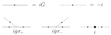
Figure 9: Feynman rules for the expansion around two spatial dimensions from the Lagrangian density in Eq. (109). The first line gives propagators, while the second line gives vertices.

V.2 Power counting rule of $\bar{\epsilon}$

We can construct the similar power counting rule of $\bar{\epsilon}$ as in the case of the expansion around four spatial dimensions. Let us first consider Feynman diagrams constructed only from $\mathcal{\bar{L}}_{0}$ and $\mathcal{\bar{L}}_{1}$, without the vertices from $\mathcal{\bar{L}}_{2}$. We make a prior assumption $\phi_{0}/\mu\sim e^{-1/\bar{\epsilon}}$, which will be checked later, and consider $\mu$ to be $O(1)$. Since $e^{-1/\bar{\epsilon}}$ is exponentially small compared to any powers of $\bar{\epsilon}$, we can neglect the contribution of $\phi_{0}$ when we expand physical observables in powers of $\bar{\epsilon}$. Then, since each pair of fermion and $\varphi$ vertices brings a factor of $\bar{\epsilon}$, the power of $\bar{\epsilon}$ for a given diagram is naively $N_{\bar{g}}/2$, where $N_{\bar{g}}$ is the number of couplings $\bar{g}$ from $\mathcal{\bar{L}}_{1}$. However, this naive power counting does not take into account the possibility of inverse powers of $\bar{\epsilon}$ from loop integrals which are logarithmically divergent at $d=2$. Let us identify diagrams which have this divergence.

Consider a diagram with $L$ loop integrals, $P_{\mathrm{F}}$ fermion propagators, and $P_{\mathrm{B}}$ internal auxiliary field lines. Each momentum loop integral in the ultraviolet region behaves as

$$\int dp_{0}d{\bm{p}}\sim\int d{\bm{p}}\,\varepsilon_{\bm{p}}\sim p^{4},$$ (115)

while each fermion propagator falls at least as $\bar{G}(p)\sim p^{-2}$ or faster. Therefore, the superficial degree of divergence the diagram has is

$$\mathcal{D}=4L-2P_{\mathrm{F}}.$$ (116)

Using the similar relations to Eq. (34), which involve the number of external fermion (auxiliary field) lines $E_{\mathrm{F(B)}}$,

$$\begin{split}L&=P_{\mathrm{F}}+P_{\mathrm{B}}-N_{\bar{g}}+1,\\ N_{g}&=P_{\mathrm{F}}+\frac{E_{\mathrm{F}}}{2}=2P_{\mathrm{B}}+E_{\mathrm{B}},\end{split}$$ (117)

the superficial degree of divergence can be written as

$$\mathcal{D}=4-E_{\mathrm{F}}-2E_{\mathrm{B}}.$$ (118)

This shows that the inverse powers of $\bar{\epsilon}$ appear only in diagrams where $E_{\mathrm{F}}+2E_{\mathrm{B}}\leq 4$ is satisfied. Moreover, from the analytic properties of $G(p)$ in the ultraviolet region discussed in Eq. (36), one can show that there are only two skeleton diagrams which have the $1/\bar{\epsilon}$ singularity near $d=2$. They are one-loop diagrams of the boson self-energy [Fig. 10(a)], and the $\varphi$ tadpole diagram [Fig. 10(c)]. We shall examine these apparent two exceptions of the naive power counting rule of $\bar{\epsilon}$.

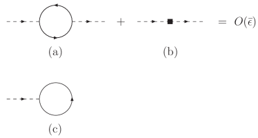
Figure 10: Two apparent exceptions of naive power counting rule of $\bar{\epsilon}$, [(a), (c)]. The boson self-energy diagram (a) is combined with the vertex from $\mathcal{\bar{L}}_{2}$ (b) to restore the naive $\bar{\epsilon}$ power counting. The condition of disappearance of the tadpole diagram (c) gives the gap equation to determine the value of condensate $\phi_{0}$.

The boson self-energy diagram in Fig. 10(a) is evaluated as

$$-i\bar{\Pi}_{\mathrm{a}}(p) =-\bar{g}^{2}\int\!\frac{dk}{(2\pi)^{d+1}}\,G_{11}\!\left(k+\frac{p}{2}\right)G_{22}\!\left(k-\frac{p}{2}\right)$$

$$=i\bar{g}^{2}\int_{\bm{k}}\frac{\theta(\varepsilon_{{\bm{k}}+\frac{{\bm{p}}}{2}}-\mu)-\theta(\mu-\varepsilon_{{\bm{k}}-\frac{{\bm{p}}}{2}})}{2\varepsilon_{\bm{k}}-(p_{0}-\frac{1}{2}\varepsilon_{\bm{p}}+2\mu+i\delta)},$$ (119)

where we have neglected the contribution of $\phi_{0}$. The integral over ${\bm{k}}$ is logarithmically divergent at $d=2$ and has a pole at $\bar{\epsilon}=0$. Thus $\bar{\Pi}_{\mathrm{a}}(p)$ is $O(1)$ instead of $O(\bar{\epsilon})$ according to the naive power counting. The residue at the pole can be computed as

$$\bar{\Pi}_{\mathrm{a}}(p) =-\bar{g}^{2}\int_{\bm{k}}\frac{1}{2\varepsilon_{\bm{k}}-(p_{0}-\frac{1}{2}\varepsilon_{\bm{p}}+2\mu+i\delta)}+\cdots$$

$$=1+O(\bar{\epsilon}),$$ (120)

and is canceled out exactly by adding the vertex $\bar{\Pi}_{0}=-1$ in $\mathcal{\bar{L}}_{2}$. Therefore the diagram of the type in Fig. 10(a) should be combined with the vertex from $\mathcal{\bar{L}}_{2}$ in Fig. 10(b) to restore the naive $\bar{\epsilon}$ power counting result, i.e., $O(\bar{\epsilon})$.

Similarly, the tadpole diagram in Fig. 10(c) also contains a $1/\bar{\epsilon}$ singularity. The requirement that this tadpole diagram should vanish by itself gives the gap equation to the leading order that determines the condensate $\phi_{0}$ as we will see in the succeeding subsection.

V.3 Gap equation

The condensate $\phi_{0}$ as a function of the chemical potential $\mu$ is determined by the gap equation which is obtained by the condition of the disappearance of all tadpole diagrams. The leading contribution to the gap equation is the one-loop diagram drawn in Fig. 10(c), which is given by

$$\bar{\Xi}_{1}=\bar{g}\int\!\frac{dk}{(2\pi)^{d+1}}\,G_{21}(k)=i\bar{g}\int_{\bm{k}}\frac{\phi_{0}}{2\bar{E}_{\bm{k}}}.$$ (121)

By changing the integration variable to $z=\varepsilon_{\bm{k}}/\mu$, we obtain

$$\begin{split}\bar{\Xi}_{1}&=\frac{i\bar{g}\phi_{0}}{2\mu}\frac{\left(\frac{m\mu}{2\pi}\right)^{\frac{d}{2}}}{\Gamma\!\left(\frac{d}{2}\right)}\int_{0}^{\infty}\!dz\,\frac{z^{\bar{\epsilon}/2}}{\sqrt{(z-1)^{2}+(\phi_{0}/\mu)^{2}}}.\end{split}$$ (122)

The integration over $z$ in the dimensional regularization can be performed to lead to

$$\bar{\Xi}_{1}=\frac{i\bar{g}\phi_{0}}{\mu}\frac{\left(\frac{m\mu}{2\pi}\right)^{\frac{d}{2}}}{\Gamma\!\left(\frac{d}{2}\right)}\left[\ln\frac{2\mu}{\phi_{0}}-\frac{1}{\bar{\epsilon}}+O(\bar{\epsilon}^{2})\right].$$ (123)

The first term $\ln 2\mu/\phi_{0}$ originates from the singularity around the Fermi surface as is well known as the Cooper instability, while the second term $1/\bar{\epsilon}$ is from the logarithmic singularity of the ${\bm{k}}$ integration at $d=2$ in $\bar{\Xi}_{1}$. Solving the gap equation $\bar{\Xi}_{1}=0$, we obtain the condensate as $\phi_{0}=2\mu\,e^{-1/\bar{\epsilon}}$. Note that this result is equivalent to that obtained by the mean field BCS theory.

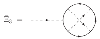
Figure 11: The tadpole diagram which gives the medium-effect correction to the gap equation.

It is known that the preexponential factor in the mean field result $\phi_{0}=2\mu\,e^{-1/\bar{\epsilon}}$ is modified due to the effects of medium gorkov ; heiselberg . In the language of the tadpole diagrams, the corresponding modification to the gap equation comes from the three-loop diagram $\bar{\Xi}_{3}$ depicted in Fig. 11. The diagram, which seems proportional to $g^{4}\sim\bar{\epsilon}^{2}$, turns out to give the $O(1)$ correction to the gap equation.

Using the Feynman rules, the tadpole diagram in Fig. 11 is given by

$$\bar{\Xi}_{3} =-\bar{g}^{5}\int\!\frac{dk\,dp\,dq}{(2\pi)^{3d+3}}\mathop{\mathrm{Tr}}\!\left[\bar{G}\sigma_{+}\bar{G}\sigma_{-}\bar{G}\sigma_{+}\bar{G}\sigma_{+}\bar{G}\sigma_{-}\right]$$

$$\begin{split}&=-\bar{g}^{5}\int\!\frac{dk\,dp\,dq}{(2\pi)^{3d+3}}\,\bar{G}_{11}(p)\,\bar{G}_{22}(p)\\ &\qquad\qquad\times\bar{G}_{11}(p-k)\,\bar{G}_{21}(q)\,\bar{G}_{22}(q+k).\end{split}$$ (124)

Since the second term in the product,

$$\bar{G}_{11}(p)\,\bar{G}_{22}(p)=\frac{1}{p_{0}^{\,2}-\bar{E}_{\bm{p}}^{\,2}}+\frac{\phi_{0}^{\,2}}{(p_{0}^{\,2}-\bar{E}_{\bm{p}}^{\,2})^{2}},$$ (125)

gives only the $O(\bar{\epsilon})$ correction to the gap equation, we can neglect it for the current purpose. Then we perform the integrations over $p_{0}$ and $q_{0}$ to result in

$$\bar{\Xi}_{3} =-\bar{g}^{5}\int\!\frac{dk\,d{\bm{p}}\,d{\bm{q}}}{(2\pi)^{3d+1}}\,\frac{\phi_{0}}{4\bar{E}_{\bm{p}}\bar{E}_{\bm{q}}}$$ (126)

$$\times\left[\frac{\bar{E}_{\bm{p}}-k_{0}+\varepsilon_{{\bm{p}}-{\bm{k}}}-\mu}{(\bar{E}_{\bm{p}}-k_{0})^{2}-\bar{E}_{{\bm{p}}-{\bm{k}}}^{\,2}}+\frac{\bar{E}_{\bm{p}}+\varepsilon_{\bm{p}}-\mu}{(k_{0}+\bar{E}_{\bm{p}})^{2}-\bar{E}_{{\bm{p}}+{\bm{k}}}^{\,2}}\right]$$

$$\times\left[\frac{k_{0}+\bar{E}_{\bm{q}}-\varepsilon_{{\bm{q}}+{\bm{k}}}+\mu}{(k_{0}+\bar{E}_{\bm{q}})^{2}-\bar{E}_{{\bm{q}}+{\bm{k}}}^{\,2}}+\frac{\bar{E}_{\bm{q}}-\varepsilon_{\bm{q}}+\mu}{(k_{0}-\bar{E}_{\bm{q}})^{2}-\bar{E}_{{\bm{q}}-{\bm{k}}}^{\,2}}\right].$$

Because of the factor $1/\bar{E}_{\bm{p}}\bar{E}_{\bm{q}}$ in the integrand, the integrations over ${\bm{p}}$ and ${\bm{q}}$ are dominated around the Fermi surface where $\varepsilon_{{\bm{p}}({\bm{q}})}\sim\mu$ and hence $\bar{E}_{{\bm{p}}({\bm{q}})}\sim\phi_{0}\ll\mu$. Keeping only the dominant part in the integrand, we can write the integral as

$$\bar{\Xi}_{3} \simeq\bar{g}^{5}\int\!\frac{dk\,d{\bm{p}}\,d{\bm{q}}}{(2\pi)^{3d+1}}\,\frac{\phi_{0}}{4\bar{E}_{\bm{p}}\bar{E}_{\bm{q}}}$$ (127)

$$\qquad\left.\times\frac{1}{(k_{0}+\varepsilon_{{\bm{p}}-{\bm{k}}}-\mu)(k_{0}+\varepsilon_{{\bm{q}}+{\bm{k}}}-\mu)}\right|_{\varepsilon_{{\bm{p}}({\bm{q}})}=\mu}.$$

Now the integration over $k_{0}$ can be performed easily to lead to

$$\begin{split}\bar{\Xi}_{3}&=-i\frac{\bar{g}^{5}}{2}\phi_{0}\int_{{\bm{p}}{\bm{q}}}\frac{1}{\bar{E}_{\bm{p}}\bar{E}_{\bm{q}}}\\ &\qquad\times\int_{\bm{k}}\left.\frac{\theta(\varepsilon_{{\bm{q}}+{\bm{k}}}-\mu)\,\theta(\mu-\varepsilon_{{\bm{p}}-{\bm{k}}})}{\varepsilon_{{\bm{q}}+{\bm{k}}}-\varepsilon_{{\bm{p}}-{\bm{k}}}}\right|_{\varepsilon_{{\bm{p}}({\bm{q}})}=\mu}.\end{split}$$ (128)

If we evaluated the ${\bm{k}}$ integration in the second line at $d=3$, we would obtain the static Lindhard function representing the medium-induced interaction.

Here we shall evaluate $\bar{\Xi}_{3}$ at $d=2$. Changing the integration variables to $\varepsilon_{\bm{p}}$, $\varepsilon_{\bm{q}}$, $\varepsilon_{\bm{k}}$, $\cos\chi_{p}=\hat{\bm{k}}\cdot\hat{\bm{p}}$, $\cos\chi_{q}=\hat{\bm{k}}\cdot\hat{\bm{q}}$, and performing the integrations over $\varepsilon_{\bm{p}}$ and $\varepsilon_{\bm{q}}$, we obtain

$$\bar{\Xi}_{3} \simeq-i\frac{\bar{g}^{5}}{2}\phi_{0}\left(\frac{m}{2\pi}\right)^{3}\left(2\ln\frac{\mu}{\phi_{0}}\right)^{2}$$ (129)

$$\times\int\!\frac{d\varepsilon_{\bm{k}}\,d\chi_{p}\,d\chi_{q}}{\pi^{2}}\left.\frac{\theta(\varepsilon_{{\bm{q}}+{\bm{k}}}-\mu)\,\theta(\mu-\varepsilon_{{\bm{p}}-{\bm{k}}})}{\varepsilon_{{\bm{q}}+{\bm{k}}}-\varepsilon_{{\bm{p}}-{\bm{k}}}}\right|_{\varepsilon_{{\bm{p}}({\bm{q}})}=\mu}.$$

The range of the integrations over $\chi_{p}$ and $\chi_{q}$ are from $0$ to $\pi$. Since $\phi_{0}/\mu\propto e^{-1/\bar{\epsilon}}$, we have $(2\ln\mu/\phi_{0})^{2}\sim(2/\bar{\epsilon})^{2}$ which cancels $\bar{\epsilon}^{2}$ coming from the four vertex couplings $\bar{g}^{4}$. Finally the remaining integrations can be performed as follows:

$$\begin{split}&\int\!\frac{d\varepsilon_{\bm{k}}\,d\chi_{p}\,d\chi_{q}}{\pi^{2}}\left.\frac{\theta(\varepsilon_{{\bm{q}}+{\bm{k}}}-\mu)\,\theta(\mu-\varepsilon_{{\bm{p}}-{\bm{k}}})}{\varepsilon_{{\bm{q}}+{\bm{k}}}-\varepsilon_{{\bm{p}}-{\bm{k}}}}\right|_{\varepsilon_{{\bm{p}}({\bm{q}})}=\mu}\\ &=\left[\int_{0}^{4\mu\cos^{2}\!\chi_{p}}\!d\varepsilon_{\bm{k}}\int_{0}^{\pi/2}\!\frac{d\chi_{p}}{\pi}\int_{0}^{\pi/2}\!\frac{d\chi_{q}}{\pi}+\int_{4\mu\cos^{2}\!\chi_{q}}^{4\mu\cos^{2}\!\chi_{p}}\!d\varepsilon_{\bm{k}}\int_{0}^{\pi/2}\!\frac{d\chi_{p}}{\pi}\int_{\pi/2}^{\pi-\chi_{p}}\!\frac{d\chi_{q}}{\pi}\right]\frac{1}{2\sqrt{\mu\varepsilon_{\bm{k}}}\left(\cos\chi_{p}+\cos\chi_{q}\right)}\\ &=\frac{1}{2}\,,\end{split}$$ (130)

which gives $\bar{\Xi}_{3}$ as

$$\bar{\Xi}_{3}\simeq-i\bar{g}\phi_{0}\frac{m}{2\pi}.$$ (131)

Consequently, the gap equation $\bar{\Xi}_{1}+\bar{\Xi}_{3}=0$, which receives the $O(1)$ correction due to $\bar{\Xi}_{3}$, is modified as

$$\ln\frac{2\mu}{\phi_{0}}-\frac{1}{\bar{\epsilon}}-1+O(\bar{\epsilon})=0.$$ (132)

The solution of the gap equation becomes

$$\phi_{0}=2\mu\,\exp\!\left[-\frac{1}{\bar{\epsilon}}-1+O(\bar{\epsilon})\right]=\frac{2\mu}{e}\left[1+O(\bar{\epsilon})\right]e^{-1/\bar{\epsilon}},$$ (133)

where the value of condensate is reduced by the factor $e\approx 2.71828$. The reduction of the preexponential factor due to the medium effects is known as the Gor’kov–Melik-Barkhudarov correction at $d=3$ theories gorkov ; heiselberg .

V.4 Thermodynamic quantities

The value of the effective potential $V_{\mathrm{eff}}$ at its minimum determines the pressure $P=-\bar{V}_{\mathrm{eff}}(\phi_{0})$ at a given chemical potential $\mu$. Since the energy gain due to the superfluidity $\phi_{0}^{\,2}\sim e^{-2/\bar{\epsilon}}$ is exponentially small compared to any power series of $\bar{\epsilon}$, we can simply neglect the contribution of $\phi_{0}$ to the pressure. Up to the next-to-leading order, the effective potential receives contributions from two vacuum diagrams drawn in Fig. 12: fermion loops without and with an exchange of the auxiliary field. The one-loop diagram is $O(1)$ and given by

$$\bar{V}_{1}(0)=-2\int_{\bm{p}}\left(\mu-\varepsilon_{\bm{p}}\right)_{>}=-\frac{2\mu\left(\frac{m\mu}{2\pi}\right)^{\frac{d}{2}}}{\Gamma\!\left(\frac{d}{2}+2\right)}\equiv-P_{\mathrm{free}},$$ (134)

which represents the contribution of free fermions to the pressure. The two-loop diagram is $O(\bar{\epsilon})$, which represents the density-density correlation as

$$\begin{split}\bar{V}_{2}(0)&=-\bar{g}^{2}\int\!\frac{dp\,dq}{(2\pi)^{2d+2}}\,\bar{G}_{11}(p)\bar{G}_{22}(q)\\ &=-\bar{g}^{2}\left[\int_{\bm{p}}\theta(\mu-\varepsilon_{\bm{p}})\right]^{2}=-\epsilon\frac{\mu\left(\frac{m\mu}{2\pi}\right)^{\frac{d}{2}}}{\Gamma\!\left(\frac{d}{2}+1\right)^{2}}.\end{split}$$ (135)

Thus we obtain the pressure up to the next-to-leading order in $\bar{\epsilon}$ as

$$P=\left(1+\bar{\epsilon}\right)P_{\mathrm{free}}.$$ (136)

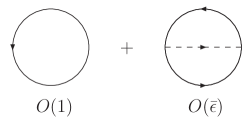
Figure 12: Vacuum diagrams contributing to the pressure up to the next-to-leading order in $\bar{\epsilon}$.

Accordingly, the fermion number density is given by $N=\partial P/\partial\mu=\left(1+\bar{\epsilon}\right)N_{\mathrm{free}}$. The Fermi energy is obtained from the thermodynamics of free gas in $d$ spatial dimension as

$$\varepsilon_{\mathrm{F}}=\frac{2\pi}{m}\left[\frac{1}{2}\,\Gamma\!\left(\frac{d}{2}+1\right)N\right]^{2/d}=\left(1+\bar{\epsilon}\right)\mu,$$ (137)

which yields the universal parameter of the unitary Fermi gas from the $\bar{\epsilon}$ expansion as

$$\xi=\frac{\mu}{\varepsilon_{\mathrm{F}}}=1-\bar{\epsilon}+O(\bar{\epsilon}^{2}).$$ (138)

The $O(\bar{\epsilon}^{2})$ correction to $\xi$ was recently computed to obtain $1.52\,\bar{\epsilon}^{2}$ Nishida-thesis .

V.5 Quasiparticle spectrum

To the leading order in $\bar{\epsilon}$, the dispersion relation of the fermion quasiparticle is given by $\omega_{\mathrm{F}}({\bm{p}})=\bar{E}_{\bm{p}}=\sqrt{(\varepsilon_{\bm{p}}-\mu)^{2}+\phi_{0}^{\,2}}$, which has the same form as that in the mean field BCS theory. There exist the next-to-leading-order corrections to the fermion quasiparticle spectrum from the one-loop self-energy diagrams $-i\bar{\Sigma}(p)$ depicted in Fig. 13. These corrections are only to the diagonal elements of the self-energy and each element is evaluated as

$$\begin{split}\bar{\Sigma}_{11}(p)&=-i\bar{g}^{2}\int\!\frac{dk}{(2\pi)^{d+1}}\,\bar{G}_{22}(k)\\ &=-\bar{g}^{2}\int_{\bm{k}}\theta(\mu-\varepsilon_{\bm{k}})=-\bar{\epsilon}\mu,\end{split}$$ (139)

and

$$\begin{split}\bar{\Sigma}_{22}(p)&=-i\bar{g}^{2}\int\!\frac{dk}{(2\pi)^{d+1}}\,\bar{G}_{11}(k)\\ &=\bar{g}^{2}\int_{\bm{k}}\theta(\mu-\varepsilon_{\bm{k}})=\bar{\epsilon}\mu.\end{split}$$ (140)

To this order, the self-energy is momentum independent, which effectively shifts the chemical potential due to the interaction with the other component of fermions.

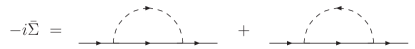
Figure 13: One-loop diagrams contributing to the fermion self-energy to order $O(\bar{\epsilon})$.

By solving the equation $\det[\bar{G}^{-1}(\omega,{\bm{p}})-\bar{\Sigma}]=0$ in terms of $\omega$, the dispersion relation of the fermion quasiparticle up to the next-to-leading order is given by

$$\omega_{\mathrm{F}}({\bm{p}})=\sqrt{(\varepsilon_{\bm{p}}-\mu-\bar{\epsilon}\mu)^{2}+\phi_{0}^{\,2}}.$$ (141)

The minimum of the dispersion curve is located at a nonzero value of momentum, $|{\bm{p}}|=(2m\varepsilon_{0})^{1/2}$, where

$$\varepsilon_{0}=\left(1+\bar{\epsilon}\right)\mu.$$ (142)

The location of the minimum coincides with the Fermi energy in Eq. (137), $\varepsilon_{0}=\varepsilon_{\mathrm{F}}$, in agreement with the Luttinger theorem luttinger . The energy gap $\Delta$ of the fermion quasiparticle is given by the condensate,

$$\Delta=\phi_{0}=\frac{2\mu}{e}\,e^{-1/\bar{\epsilon}}.$$ (143)

V.6 Extrapolation to $\bar{\epsilon}$=1

Now we discuss the extrapolation of the series expansion over $\bar{\epsilon}=d-2$ to the physical case in three spatial dimensions. In contradiction to the case of the $\epsilon=4-d$ expansion, the coefficients of the $O(\bar{\epsilon})$ corrections are not small compared to the leading terms. If we naively extrapolate the leading and next-to-leading-order results for $\xi$ in Eq. (138), $\Delta$ in Eq. (143), and $\varepsilon_{0}$ in Eq. (142) to $\bar{\epsilon}=1$, we would have

$$\xi\approx 0,\qquad\frac{\Delta}{\mu}\approx 0.271,\qquad\frac{\varepsilon_{0}}{\mu}\approx 2,$$ (144)

which are not as good as the extrapolations in the expansions over $\epsilon$ in Eq. (78). This may be related to the fact that the series expansion over $\bar{\epsilon}=d-2$ is an asymptotic series and is not Borel summable. Thus, instead of naively extrapolating the $\bar{\epsilon}$ expansions to $d=3$, we use them as boundary conditions to improve the series summation of the $\epsilon$ expansions in Sec. VI.

V.7 Large-order behavior

Here we show that the series expansion over $\bar{\epsilon}=d-2$ is not convergent, but an asymptotic series. Its physical reason is obvious: The unitary Fermi gas at $d\leq 2$ is just a free gas while the ground state at $d>2$ is the superfluid. Therefore, the radius of convergence in the expansion around two spatial dimensions is zero. In the language of the perturbation theory developed in this section, the asymptotic nature of the expansion over $\bar{\epsilon}=d-2$ can be understood by the existence of a type of diagrams which grows as $n!$ by itself at order $\bar{\epsilon}^{n}$. Such a factorial contribution originates from the low momentum integration region which resembles the infrared renormalon in the relativistic field theories Parisi ; David .

The $n+1$-loop diagram contributing to the effective potential as $n!$ at $O(\bar{\epsilon}^{n})$ is depicted in Fig. 14, which is written as

$$\bar{V}_{n+1} =\frac{i}{n}\int\!\frac{dp}{(2\pi)^{d+1}}$$ (145)

$$\times\left[1+\bar{g}^{2}\int_{\bm{k}}\frac{\theta(\varepsilon_{{\bm{k}}+\frac{{\bm{p}}}{2}}-\mu)-\theta(\mu-\varepsilon_{{\bm{k}}-\frac{{\bm{p}}}{2}})}{2\varepsilon_{\bm{k}}-(p_{0}-\frac{1}{2}\varepsilon_{\bm{p}}+2\mu+i\delta)}\right]^{n},$$

where $k_{0}$ integrations in each bubble diagram are already performed. Note that $+1$ in the bracket comes from the countervertex $-\bar{\Pi}_{0}=1$. Since the $n!$ contribution comes from the infrared region of $p$, we concentrate on the integration region where $|p_{0}|\ll\mu$ and $\varepsilon_{\bm{p}}\ll\mu$. Rotating the contour of the $p_{0}$ integration to the imaginary axis, $p_{0}\to i\tilde{p}_{0}$ (Wick rotation), the ${\bm{k}}$ integration in the bracket can be evaluated as

$$\begin{split}&1+\bar{g}^{2}\int_{\bm{k}}\frac{\theta(\varepsilon_{{\bm{k}}+\frac{{\bm{p}}}{2}}-\mu)-\theta(\mu-\varepsilon_{{\bm{k}}-\frac{{\bm{p}}}{2}})}{2\varepsilon_{\bm{k}}-(p_{0}-\frac{1}{2}\varepsilon_{\bm{p}}+2\mu+i\delta)}\\ &=-\bar{\epsilon}\,\ln\!\left(\frac{|\tilde{p}_{0}|}{4\mu}+\sqrt{\left(\frac{\tilde{p}_{0}}{4\mu}\right)^{2}+\frac{\varepsilon_{\bm{p}}}{4\mu}}\right)+\cdots.\end{split}$$ (146)

Here $\cdots$ includes higher order terms in $\bar{\epsilon}$ and regular dependences on $\tilde{p}_{0}$ and $\varepsilon_{\bm{p}}$. The logarithmic dependence on $\tilde{p}_{0}$ and $\varepsilon_{\bm{p}}$ appears due to the singularity of the ${\bm{k}}$ integration near the Fermi surface $\varepsilon_{\bm{k}}\sim\mu$ in the limit $p\to 0$. Such a logarithmic term dominates the $p$ integration when $p$ is small. Collecting the logarithmic term from each bracket, the $\tilde{p}_{0}$ and ${\bm{p}}$ integrals in Eq. (145) at their low momentum regions contribute to $\bar{V}_{n+1}$ as

$$\bar{V}_{n+1} \sim\frac{1}{n}\int_{0}d\tilde{p}_{0}d{\bm{p}}\left[-\bar{\epsilon}\,\ln\!\left(\frac{|\tilde{p}_{0}|}{4\mu}+\sqrt{\left(\frac{\tilde{p}_{0}}{4\mu}\right)^{2}+\frac{\varepsilon_{\bm{p}}}{4\mu}}\right)\right]^{n}$$

$$\sim\left(\frac{\bar{\epsilon}}{3}\right)^{n}\Gamma(n),$$ (147)

which behaves as the factorial of $n$.

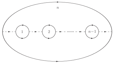
Figure 14: An $n$th order diagram at $d=2$ which contributes to the pressure as $n!$ by itself. The countervertex $-i\bar{\Pi}_{0}=i$ for each bubble diagram is understood implicitly.

Because the large-order contribution grows up with the same sign, it produces the singularity on the real positive axis of the Borel transform. Thus the expansion over $\bar{\epsilon}=d-2$ is not Borel summable and its Borel transformation will have the inevitable ambiguity $\sim e^{-3/\bar{\epsilon}}$, indicating that the ground state where the expansion is performed is unstable. Finally, it is important to note that the discussion here is not applicable to the expansion around $d=4$ because the singularity near the Fermi surface is cured by the existence of the large condensate $\phi_{0}\gg\mu$. In the Appendix A, we explicitly demonstrate that the diagrams in Fig. 14 do not yield a factorial growth in the coefficients of the $\epsilon$ expansion.

VI Matching of expansions around four and two spatial dimensions

As we have mentioned previously, we shall match the two expansions around $d=4$ and $d=2$, which were studied in Secs. III and V, respectively, in order to extract results at $d=3$. We use the results around two spatial dimensions as boundary conditions which should be satisfied by the series summations of the expansions over $\epsilon=4-d$. Because we do not yet have a precise knowledge of the large-order behavior of the expansion around four spatial dimensions, we assume its Borel summability and employ Padé approximants.

Let us demonstrate the matching of the two expansions by taking $\xi$ as an example. In Ref. nussinov04 , the linear interpolation between the exact values at $d=2$ $(\xi=1)$ and $d=4$ $(\xi=0)$ was discussed to yield $\xi=0.5$ at $d=3$. Now we have series expansions around these two exact limits. The expansion of $\xi$ in terms of $\epsilon=4-d$ is obtained in Eq. (62). Assuming the Borel summability of the $\epsilon$ expansion, we write $\xi$ as a function of $\epsilon$ in the form of the Borel transformation,

$$\xi(\epsilon)=\frac{\epsilon^{3/2}}{2}\exp\!\left(\frac{\epsilon\ln\epsilon}{8-2\epsilon}\right)\int_{0}^{\infty}\!dt\,e^{-t}B_{\xi}(\epsilon t),$$ (148)

where we factorized out the trivial nonanalytic dependences on $\epsilon$ explicitly. $B_{\xi}(t)$ is the Borel transform of the power series in $\xi(\epsilon)$, whose Taylor coefficients at origin are given from the $\epsilon$ expansion of $\xi$ as

$$B_{\xi}(t)=1-\left(3C-\frac{5}{4}(1-\ln 2)\right)t+\cdots.$$ (149)

In order to perform the integration over $t$ in Eq. (148), the analytic continuation of the Borel transform $B_{\xi}(t)$ to the real positive axis of $t$ is necessary. Here we employ the Padé approximant, where $B_{\xi}(t)$ is replaced by the following rational functions:

$$B_{\xi}(t)=\frac{1+p_{1}t+\cdots+p_{M}t^{M}}{1+q_{1}t+\cdots+q_{N}t^{N}}\,.$$ (150)

From Eq. (149), we require that the Padé approximants satisfy $p_{1}-q_{1}=-3C+\frac{5}{4}(1-\ln 2)$. Furthermore, we incorporate the results around two spatial dimensions in Eq. (138) by imposing

$$\xi(2-\bar{\epsilon})=1-\bar{\epsilon}+\cdots$$ (151)

on the Padé approximants as a boundary condition. Since we have three known coefficients from the two expansions, the Padé approximants $[M/N]$ satisfying $M+N=3$ are possible. Since we could not find a solution satisfying the boundary condition $\xi(2-\bar{\epsilon})=1-\bar{\epsilon}$ for $[M/N]=[2/1]$, we adopt three other Padé approximants with $[M/N]=[3/0],\,[1/2],\,[0/3]$, whose coefficients $p_{m}$ and $q_{n}$ are determined uniquely by the above conditions.

Figure 15 shows the universal parameter $\xi$ as a function of the spatial dimension $d$. The middle three curves show $\xi$ in the different Padé approximants connecting the two expansions around $d=4$ and $d=2$. These Borel-Padé approximations give $\xi=0.391$, $0.364$, and $0.378$ at $d=3$, which are small compared to the naive extrapolation of the $\epsilon$ expansion to $d=3$ $(\xi\to 0.475)$.

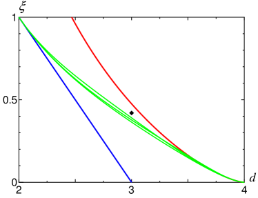
Figure 15: (Color online) The universal parameter $\xi$ as a function of the spatial dimensions $d$. The upper solid curve is from the expansion around $d=4$ in Eq. (62), while the lower solid line is from the expansion around $d=2$ in Eq. (138). The middle three curves show the different Borel-Padé approximations connecting the two expansions. The diamond indicates the result $\xi\approx 0.42$ from the Monte Carlo simulation Carlson:2005kg .

The Padé approximant above, however, almost certainly needs serious modification, since we can show that in the expansion of $\xi(\epsilon)$, there exist nonanalytic terms at sufficiently higher orders in $\epsilon$,

$$\begin{split}\xi(\epsilon)&=\frac{\epsilon^{3/2}}{2}\exp\left(\frac{\epsilon\ln\epsilon}{8-2\epsilon}\right)\\ &\quad\times\left(1-0.0492\epsilon+\#\,\epsilon^{2}+\#\,\epsilon^{3}\ln\epsilon+\cdots\right).\end{split}$$ (152)

The nonanalytic term at $O(\epsilon^{3})$ compared to the leading order originates from a resummation of boson self-energies to avoid infrared singularities. An understanding of the analytic structure of high-order terms in the perturbation theory around $d=4$ is currently lacking.

VII Summary and concluding remarks

We have developed the systematic expansion for the Fermi gas near the unitarity limit treating the dimensionality of space $d$ as close to four. To the leading and next-to-leading orders in the expansion over $\epsilon=4-d$, the thermodynamic quantities and the fermion quasiparticle spectrum were calculated as functions of the binding energy $\varepsilon_{\mathrm{b}}$ of the two-body state. Results for the physical case of three spatial dimensions were obtained by extrapolating the series expansions to $\epsilon=1$. The pressure, energy density, and chemical potential in the unitary regime at fixed density were found to be

$$\frac{P}{\varepsilon_{\mathrm{F}}N} =\frac{2}{d+2}\,\xi-\frac{\epsilon}{4}\frac{\varepsilon_{\mathrm{b}}}{2\varepsilon_{\mathrm{F}}},$$ (153)

$$\frac{E}{\varepsilon_{\mathrm{F}}N} =\frac{d}{d+2}\,\xi-\frac{\varepsilon_{\mathrm{b}}}{2\varepsilon_{\mathrm{F}}}\left(1+\frac{\epsilon}{4}+\frac{\epsilon\ln\epsilon}{4}-\frac{\epsilon}{2}\ln\frac{\varepsilon_{\mathrm{b}}}{\varepsilon_{\mathrm{F}}}\right),\phantom{\frac{\frac{\int}{\int}}{\frac{\int}{\int}}}$$ (154)

$$\frac{\mu}{\varepsilon_{\mathrm{F}}} =\xi-\frac{\varepsilon_{\mathrm{b}}}{2\varepsilon_{\mathrm{F}}}\left(1+\frac{\epsilon}{2}+\frac{\epsilon\ln\epsilon}{4}-\frac{\epsilon}{2}\ln\frac{\varepsilon_{\mathrm{b}}}{\varepsilon_{\mathrm{F}}}\right),$$ (155)

where

$$\xi=\frac{\epsilon^{3/2}}{2}+\frac{\epsilon^{5/2}}{16}\ln\epsilon-0.0246\,\epsilon^{5/2}+O(\epsilon^{7/2})\approx 0.475$$ (156)

is the universal parameter of the unitary Fermi gas. The fermion quasiparticle spectrum around its minimum in the unitarity limit was given by the form $\omega_{\mathrm{F}}({\bm{p}})\simeq\sqrt{(\varepsilon_{\bm{p}}-\varepsilon_{0})^{2}+\Delta^{2}}$ with the energy gap

$$\frac{\Delta}{\mu}=\frac{2}{\epsilon}-0.691+O(\epsilon)\approx 1.31$$ (157)

and the location of the minimum of the dispersion curve

$$\frac{\varepsilon_{0}}{\mu}=2+O(\epsilon)\approx 2.$$ (158)

Although we have only the first two terms in the $\epsilon$ expansion, these extrapolated values give reasonable results consistent with the Monte Carlo simulations or the experimental measurements. Furthermore, the next-to-leading-order corrections are not too large even at $\epsilon=1$, which suggests that the picture of the unitary Fermi gas as a collection of weakly interacting fermionic and bosonic quasiparticles may be a useful starting point even in three spatial dimensions.

We have also formulated the systematic expansion for the unitary Fermi gas around two spatial dimensions. We used the results around $d=2$ as boundary conditions which should be satisfied by the series summations of the expansion over $\epsilon=4-d$. The simple Borel-Padé approximations connecting the two expansions yielded $\xi=0.378\pm 0.013$ at $d=3$, which is small compared to the naive extrapolation of the $\epsilon$ expansion (Fig. 15). In order for the accurate determination of $\xi$ at $d=3$, the precise knowledge on the large-order behavior of the expansion around four spatial dimensions as well as the calculation of higher order corrections would be desirable. Once this information becomes available, a conformal mapping technique, if applicable, will further improve the series summations justin .

The phase structure of the polarized Fermi gas in the unitary regime has been studied based on the $\epsilon$ expansion. We found the splitting point, where the minimum of the fermion dispersion curve sits exactly at zero momentum, located on the BEC side of the unitarity point where $ak_{\mathrm{F}}\approx 1$ and $\mu/\varepsilon_{\mathrm{F}}\approx-0.5$. Then the gapless superfluid phase and the superfluid phase with the spatially varying condensate were shown to exist between the gapped superfluid phase and the polarized normal phase in a certain range of the binding energy. Our study gives a microscopic foundation to the phase structure around the splitting point which has been proposed using the effective field theory son05 . Moreover, we found the gapless phase with the spatially varying condensate around $d=4$ exists only at $0.494\lesssim(ak_{\mathrm{F}})^{-1}\lesssim 1$ and terminates near the unitarity limit in contrast to the conjectured phase diagram where that phase is connected to the FFLO phase in the BCS limit son05 . Our result suggests that the superfluid phase with the spatially varying condensate existing in the unitary regime may be separated from the FFLO phase in the BCS regime. Further study will be worthwhile to confirm this possibility.

We believe that the $\epsilon$ expansion is not only theoretically interesting but also provides us an useful analytical tool to investigate the properties of the unitary Fermi gas. As far as we know, this is the only systematic expansion for the unitary Fermi gas at zero temperature that exists at this moment. The application of the $\epsilon$ expansion to study the thermodynamics of the unitary Fermi gas at finite temperature will be reported elsewhere finite-T .

Note added. Renormalization group argument to support our results appeared after we submitted our manuscript. Reference Sachdev studied a renormalization group flow equation and found the fixed point describing the unitarity limit to approach the noninteracting Gaussian fixed point in the limit $d=4$ or $d=2$. Therefore, slightly below $d=4$ or above $d=2$, the finite density system associated with the fixed point is weakly coupled. The small effective coupling in our Eq. (15) or Eq. (18) was correctly reproduced by the renormalization group fixed point Sachdev .

*

Appendix A Cancellation of renormalons at $d=4-\epsilon$

Here we discuss the ultraviolet renormalon Gross-Neveu ; Lautrup ; tHooft , which is naively present in the diagram depicted in Fig. 14 and produces a $n!$ contribution at order $\epsilon^{n}$ from the large momentum integration region of a single diagram. The purpose of this Appendix is to show that the $n!$ contribution cancels with subleading contributions from lower-order diagrams in the expansion over $\epsilon=4-d$. The $n+1$-loop diagram in Fig. 14 can be written as

$$V_{n+1}=\frac{i}{n}\int\!\frac{dp}{(2\pi)^{d+1}}\left[D(p)\left\{\Pi_{0}(p)+\Pi_{\mathrm{a}}(p)\right\}\right]^{n},$$ (159)

where $D(p)$, $\Pi_{0}(p)$, and $\Pi_{\mathrm{a}}(p)$ are, respectively, defined in Eqs. (30), (31), and (37). Introducing these definitions and integrating over $p_{0}$, we obtain the following expression for $V_{n+1}$:

$$\begin{split}V_{n+1}&=-\frac{g^{2}}{4}\int_{{\bm{p}}{\bm{k}}}\frac{(E_{{\bm{k}}-\frac{{\bm{p}}}{2}}-\varepsilon_{{\bm{k}}-\frac{{\bm{p}}}{2}})(E_{{\bm{k}}+\frac{{\bm{p}}}{2}}-\varepsilon_{{\bm{k}}+\frac{{\bm{p}}}{2}})}{E_{{\bm{k}}-\frac{{\bm{p}}}{2}}E_{{\bm{k}}+\frac{{\bm{p}}}{2}}\left(E_{{\bm{k}}-\frac{{\bm{p}}}{2}}+E_{{\bm{k}}+\frac{{\bm{p}}}{2}}+\frac{\varepsilon_{\bm{p}}}{2}\right)}\\ &\qquad\qquad\times\left[1+\frac{g^{2}}{E_{{\bm{k}}-\frac{{\bm{p}}}{2}}+E_{{\bm{k}}+\frac{{\bm{p}}}{2}}+\frac{\varepsilon_{\bm{p}}}{2}}\int_{\bm{l}}\frac{1}{4E_{{\bm{l}}-\frac{{\bm{p}}}{2}}E_{{\bm{l}}+\frac{{\bm{p}}}{2}}}\right.\\ &\qquad\qquad\qquad\quad\left.\times\left\{\frac{(E_{{\bm{l}}-\frac{{\bm{p}}}{2}}+\varepsilon_{{\bm{l}}-\frac{{\bm{p}}}{2}})(E_{{\bm{l}}+\frac{{\bm{p}}}{2}}+\varepsilon_{{\bm{l}}+\frac{{\bm{p}}}{2}})}{E_{{\bm{l}}-\frac{{\bm{p}}}{2}}+E_{{\bm{l}}+\frac{{\bm{p}}}{2}}+E_{{\bm{k}}-\frac{{\bm{p}}}{2}}+E_{{\bm{k}}+\frac{{\bm{p}}}{2}}}+\frac{(E_{{\bm{l}}-\frac{{\bm{p}}}{2}}-\varepsilon_{{\bm{l}}-\frac{{\bm{p}}}{2}})(E_{{\bm{l}}+\frac{{\bm{p}}}{2}}-\varepsilon_{{\bm{l}}+\frac{{\bm{p}}}{2}})}{E_{{\bm{l}}-\frac{{\bm{p}}}{2}}+E_{{\bm{l}}+\frac{{\bm{p}}}{2}}-E_{{\bm{k}}-\frac{{\bm{p}}}{2}}-E_{{\bm{k}}+\frac{{\bm{p}}}{2}}}\right\}\right]^{n-1}.\end{split}$$ (160)

Now we consider the ${\bm{l}}$ integration in the bracket. Since the ${\bm{l}}$ integration contains a logarithmic divergence at $d=4$, we subtract and add its divergent piece as

$$\begin{split}&1+\frac{g^{2}}{E_{{\bm{k}}-\frac{{\bm{p}}}{2}}+E_{{\bm{k}}+\frac{{\bm{p}}}{2}}+\frac{\varepsilon_{\bm{p}}}{2}}\int_{\bm{l}}\frac{1}{4E_{{\bm{l}}-\frac{{\bm{p}}}{2}}E_{{\bm{l}}+\frac{{\bm{p}}}{2}}}\biggl{\{}\ \cdots\ \biggr{\}}\\ &\qquad=\frac{g^{2}}{E_{{\bm{k}}-\frac{{\bm{p}}}{2}}+E_{{\bm{k}}+\frac{{\bm{p}}}{2}}+\frac{\varepsilon_{\bm{p}}}{2}}\int_{\bm{l}}\left[\frac{1}{4E_{{\bm{l}}-\frac{{\bm{p}}}{2}}E_{{\bm{l}}+\frac{{\bm{p}}}{2}}}\biggl{\{}\ \cdots\ \biggr{\}}-\frac{1}{2\varepsilon_{\bm{l}}+E_{{\bm{k}}-\frac{{\bm{p}}}{2}}+E_{{\bm{k}}+\frac{{\bm{p}}}{2}}+\frac{\varepsilon_{\bm{p}}}{2}}\right]\\ &\qquad\quad+1+\frac{g^{2}}{E_{{\bm{k}}-\frac{{\bm{p}}}{2}}+E_{{\bm{k}}+\frac{{\bm{p}}}{2}}+\frac{\varepsilon_{\bm{p}}}{2}}\int_{\bm{l}}\frac{1}{2\varepsilon_{\bm{l}}+E_{{\bm{k}}-\frac{{\bm{p}}}{2}}+E_{{\bm{k}}+\frac{{\bm{p}}}{2}}+\frac{\varepsilon_{\bm{p}}}{2}}.\end{split}$$ (161)

The ${\bm{l}}$ integration in the second line becomes finite at $d=4$ and does not produce singular logarithmic terms. So we concentrate on the ${\bm{l}}$ integration in the last line, which can be evaluated in the dimensional regularization as

$$1+\frac{g^{2}}{E_{{\bm{k}}-\frac{{\bm{p}}}{2}}+E_{{\bm{k}}+\frac{{\bm{p}}}{2}}+\frac{\varepsilon_{\bm{p}}}{2}}\int_{\bm{l}}\frac{1}{2\varepsilon_{\bm{l}}+E_{{\bm{k}}-\frac{{\bm{p}}}{2}}+E_{{\bm{k}}+\frac{{\bm{p}}}{2}}+\frac{\varepsilon_{\bm{p}}}{2}}=1+\frac{\epsilon}{2}\,\Gamma\!\left(1-\frac{d}{2}\right)\left(\frac{E_{{\bm{k}}-\frac{{\bm{p}}}{2}}+E_{{\bm{k}}+\frac{{\bm{p}}}{2}}+\frac{\varepsilon_{\bm{p}}}{2}}{2\phi_{0}}\right)^{-\frac{\epsilon}{2}}.$$ (162)

Then $V_{n+1}$ in Eq. (160) becomes

$$V_{n+1}=-\frac{g^{2}}{4}\int_{{\bm{p}}{\bm{q}}}\frac{(E_{\bm{p}}-\varepsilon_{\bm{p}})(E_{\bm{q}}-\varepsilon_{\bm{q}})}{E_{\bm{p}}E_{\bm{q}}\left(E_{\bm{p}}+E_{\bm{q}}+\frac{\varepsilon_{{\bm{p}}-{\bm{q}}}}{2}\right)}\left[1+\frac{\epsilon}{2}\,\Gamma\!\left(-1+\frac{\epsilon}{2}\right)\left(\frac{E_{\bm{p}}+E_{\bm{q}}+\frac{\varepsilon_{{\bm{p}}-{\bm{q}}}}{2}}{2\phi_{0}}\right)^{-\frac{\epsilon}{2}}+\mathrm{\,regular\ terms\,}\right]^{n-1},$$ (163)

where the integration valuables are redefined to be ${\bm{k}}-\frac{{\bm{p}}}{2}\to{\bm{p}}$ and ${\bm{k}}+\frac{{\bm{p}}}{2}\to{\bm{q}}$. “Regular terms” coming from the second line in Eq. (161) vanish in the limit ${\bm{p}}\to\infty$ or ${\bm{q}}\to\infty$.

If one expanded $V_{n+1}$ in powers of $\epsilon$ and picked up the logarithmic terms, one would find the ${\bm{p}}$ integration from its large momentum region $\varepsilon_{\bm{p}}\gg\phi_{0},\varepsilon_{\bm{q}}$ gives the following contribution to the effective potential at $O(\epsilon^{n})$:

$$\begin{split}V_{n+1}&=-\frac{g^{2}}{4}\int_{{\bm{p}}{\bm{q}}}\frac{(E_{\bm{p}}-\varepsilon_{\bm{p}})(E_{\bm{q}}-\varepsilon_{\bm{q}})}{E_{\bm{p}}E_{\bm{q}}\left(E_{\bm{p}}+E_{\bm{q}}+\frac{\varepsilon_{{\bm{p}}-{\bm{q}}}}{2}\right)}\left[\frac{\epsilon}{2}\,\ln\!\left(\frac{E_{\bm{p}}+E_{\bm{q}}+\frac{\varepsilon_{{\bm{p}}-{\bm{q}}}}{2}}{2\phi_{0}}\right)+\cdots\right]^{n-1}\\ &\sim\epsilon\int\!d\varepsilon_{\bm{p}}\left(\frac{1}{\varepsilon_{\bm{p}}}\right)^{2}\left(\frac{\epsilon}{2}\ln\varepsilon_{\bm{p}}\right)^{n-1}\sim\left(\frac{\epsilon}{2}\right)^{n}\Gamma(n),\end{split}$$ (164)

which grows as a factorial of $n$. Whether such a $n!$ contribution at $O(\epsilon^{n})$ really survives and dominates the large-order behavior of the perturbative expansion is a subtle problem. Actually in our case, we can show that the factorial contribution of $V_{n+1}$ at $O(\epsilon^{n})$ cancels because the lower-order diagrams $V_{i\leq n}$ also produce $n!$ contributions to $O(\epsilon^{n})$ with different signs.

In order to see the cancellation explicitly, we sum up $V_{n+1}$ in Eq. (163) over $n$ to result in

$$\sum_{n=1}^{\infty}V_{n+1}=\frac{g^{2}}{4}\int_{{\bm{p}}{\bm{q}}}\frac{(E_{\bm{p}}-\varepsilon_{\bm{p}})(E_{\bm{q}}-\varepsilon_{\bm{q}})}{E_{\bm{p}}E_{\bm{q}}\left(E_{\bm{p}}+E_{\bm{q}}+\frac{\varepsilon_{{\bm{p}}-{\bm{q}}}}{2}\right)}\left[\frac{\epsilon}{2}\,\Gamma\!\left(-1+\frac{\epsilon}{2}\right)\left(\frac{E_{\bm{p}}+E_{\bm{q}}+\frac{\varepsilon_{{\bm{p}}-{\bm{q}}}}{2}}{2\phi_{0}}\right)^{-\frac{\epsilon}{2}}+\mathrm{\,regular\ terms\,}\right]^{-1}.$$ (165)

From the large momentum region of the ${\bm{p}}$ integration, we obtain

$$\sum_{n}V_{n+1}\sim\epsilon\int\!d\varepsilon_{\bm{p}}\left(\frac{1}{\varepsilon_{\bm{p}}}\right)^{2-\frac{\epsilon}{2}}\sim\sum_{n}\left(\frac{\epsilon}{2}\right)^{n},$$ (166)

where the $n!$ contribution at $O(\epsilon^{n})$ has been canceled with the subleading contributions from the lower-order diagrams. Since the instanton contribution to the large orders, even if it exists, typically has alternating signs, the possibility of the Borel summability of the $\epsilon=4-d$ expansion, which was assumed in Sec. VI, remains open.

References

- (1) A. J. Leggett, in Modern Trends in the Theory of Condensed Matter (Springer, Berlin, 1980).
- (2) P. Nozières and S. Schmitt-Rink, J. Low Temp. Phys. 59, 195 (1985).
- (3) K. M. O’Hara et al., Science 298, 2179 (2002).
- (4) C. A. Regal, M. Greiner, and D. S. Jin, Phys. Rev. Lett. 92, 040403 (2004).
- (5) M. Bartenstein et al., Phys. Rev. Lett. 92, 120401 (2004).
- (6) M. W. Zwierlein et al., Phys. Rev. Lett. 92, 120403 (2004).
- (7) J. Kinast et al., Phys. Rev. Lett. 92, 150402 (2004).
- (8) T. Bourdel et al., Phys. Rev. Lett. 93, 050401 (2004).
- (9) J. Kinast et al., Science 307, 1296 (2005).
- (10) G. Bertsch, Many-Body X Challenge, in Proceedings of the Tenth International Conference on Recent Progress in Many-Body Theories, edited by R. F. Bishop et al. (World Scientific, Singapore, 2000).
- (11) See, e.g., Q. Chen, J. Stajic, S. Tan, and K. Levin, Phys. Rep. 412, 1 (2005), and references therein.
- (12) J. Carlson, S.-Y. Chang, V. R. Pandharipande, and K. E. Schmidt, Phys. Rev. Lett. 91, 050401 (2003); S. Y. Chang, V. R. Pandharipande, J. Carlson, and K. E. Schmidt, Phys. Rev. A 70, 043602 (2004).
- (13) J. W. Chen and D. B. Kaplan, Phys. Rev. Lett. 92, 257002 (2004).
- (14) G. E. Astrakharchik, J. Boronat, J. Casulleras, and S. Giorgini, Phys. Rev. Lett. 93, 200404 (2004).
- (15) J. Carlson and S. Reddy, Phys. Rev. Lett. 95, 060401 (2005).
- (16) Y. Nishida and D. T. Son, Phys. Rev. Lett. 97, 050403 (2006).
- (17) Z. Nussinov and S. Nussinov, arXiv:cond-mat/0410597.
- (18) G. Rupak, arXiv:nucl-th/0605074.
- (19) K. G. Wilson and J. Kogut, Phys. Rep. 12, 75 (1974).
- (20) M. W. Zwierlein, A. Schirotzek, C. H. Schunck, and W. Ketterle, Science 311, 492 (2006).
- (21) G. B. Partridge, W. Li, R. I. Kamar, Y. Liao, and R. G. Hulet, Science 311, 503 (2006).
- (22) M. W. Zwierlein, C. H. Schunck, A. Schirotzek, and W. Ketterle, Nature 442, 54 (2006).
- (23) Y. Shin, M. W. Zwierlein, C. H. Schunck, A. Schirotzek, and W. Ketterle, Phys. Rev. Lett. 97, 030401 (2006).
- (24) M. Randeria, J.-M. Duan, and L.-Y. Shieh, Phys. Rev. Lett. 62, 981 (1989); Phys. Rev. B 41, 327 (1990).
- (25) See, e.g., M. E. Peskin and D. V. Schroeder, An Introduction to Quantum Field Theory (Addison-Wesley, Reading, MA, 1995).
- (26) D. T. Son and M. A. Stephanov, Phys. Rev. A 74, 013614 (2006).
- (27) L. P. Gor’kov and T. K. Melik-Barkhudarov, Sov. Phys. JETP 13, 1018 (1961).
- (28) H. Heiselberg, C. J. Pethick, H. Smith, and L. Viverit, Phys. Rev. Lett. 85, 2418 (2000).
- (29) Y. Nishida, Ph.D. thesis, University of Tokyo, 2007 [available as arXiv:cond-mat/0703465].
- (30) J. M. Luttinger, Phys. Rev. 119, 1153 (1960).
- (31) G. Parisi, Nucl. Phys. B 150, 163 (1979).
- (32) F. David, Nucl. Phys. B 209, 433 (1982); Nucl. Phys. B 234, 237 (1984); Nucl. Phys. B 263, 637 (1986).
- (33) See, e.g., J. Zinn-Justin, Quantum Field Theory and Critical Phenomena (Clarendon Press, Oxford, 2002).
- (34) Y. Nishida, Phys. Rev. A 75, 063618 (2007).
- (35) P. Nikolic and S. Sachdev, arXiv:cond-mat/0609106.
- (36) D. J. Gross and A. Neveu, Phys. Rev. D 10, 3235 (1974).
- (37) B. Lautrup, Phys. Lett. B 69, 109 (1977).
- (38) G. ’t Hooft, in The Whys of Subnuclear Physics, Proceedings of the International School, Erice, Italy, 1977, edited by A. Zichichi (Plenum, New York, 1978).