Polarized fermions in the unitarity limit
Abstract
We consider a polarized Fermi gas in the unitarity limit. Results are calculated analytically up to next-to-leading order in an expansion about spatial dimensions. We find a first order transition from superfluid to normal phase. The critical chemical potential asymmetry for this phase transition is , where is the expansion parameter and is the average chemical potential of the two fermion species. Stability of the superfluid phase in the presence of supercurrents is also studied.
I Introduction
Recently, there has been a lot of interest in the quantum phase transition between a paired fermion superfluid and a normal Fermi liquid that occurs as the difference in the chemical potentials of the up and down spins is increased. This transition is well understood in the strong coupling Bose-Einstein condensation (BEC) and weak coupling Bardeen-Cooper-Schrieffer (BCS) limits, but the nature of the phase diagram near the BEC/BCS crossover remains to be elucidated. The BEC/BCS crossover is characterized by a divergent atom-atom scattering length. Over the last year, first results from experiments with polarized atomic systems near a Feshbach resonance have appeared Zwierlein:2005 ; Partridge:2005 ; Zwierlein:2006 .
Theoretically the regime of large scattering lengths is difficult since the standard perturbative methods are not applicable. Based on an observation by Nussinov and Nussinov Nussinov:2004 , Nishida and Son Nishida:2006br proposed an analytic method for calculating thermodynamic properties as an expansion around spatial dimensions. One starts by performing the calculation in arbitrary space dimensions and develops a perturbative expansion in . In this formalism, the Cooper pair energy is considered and the chemical potential . A next-to-leading order calculation Nishida:2006br of the superfluid gap and the equation of state agrees well with fixed node Green Function Monte Carlo Carlson2003 ; Chang2004 ; Astrakharchik2004 ; Carlson:2005kg and Euclidean Path Integral Bulgac:2005pj ; Burovski:2006 calculations. Somewhat smaller values of the energy per particle and the energy gap were obtained in the canonical Path Integral Monte Carlo calculation Lee:2005fk . For a polarized system with chemical potential difference , we expect the superfluid phase to become unstable when the asymmetry is on the order of the gap in the symmetric system sarma ; Larkin:1964 ; Fulde:1964 . Thus we will consider a situation where .
II Epsilon Expansion
The physics of the unitarity limit is captured by an effective lagrangian of point-like fermions interacting via a short-range interaction. The lagrangian is
| (1) |
where is a two-component spinor. The coupling constant is related to the scattering length. In dimensional regularization the unitarity limit corresponds to . In this limit the fermion-fermion scattering amplitude is given by
| (2) |
where . As a function of the Gamma function has poles at and the scattering amplitude vanishes at these points. Near the scattering amplitude is energy and momentum independent. For we find
| (3) |
We observe that at leading order in the scattering amplitude looks like the propagator of a boson with mass . The boson-fermion coupling is and vanishes as . This suggests that we can set up a perturbative expansion involving fermions of mass weakly coupled to bosons of mass . We can eliminate the four-fermion coupling in Eq. (1) using a a Hubbard-Stratonovich transformation. In the unitarity limit we get
where is a two-component Nambu-Gorkov field, are Pauli matrices acting in the Nambu-Gorkov space and . In the superfluid phase acquires an expectation value. We write
| (5) |
where and the scale was introduced in order to have a correctly normalized boson field. In order to get a well defined perturbative expansion we add and subtract a kinetic term for the boson field to the lagrangian. We include the kinetic term in the free part of the lagrangian
| (6) | |||||
The interacting part is
| (7) | |||||
Note that the interacting part generates self energy corrections to the boson propagator. Using Eq. (3) we can show that to leading order in these self energy corrections cancel against the negative of the kinetic term of the boson field in . We have also included the chemical potential term in . This is motivated by the fact that near the system reduces to a non-interacting Bose gas and . We will count as a quantity of .
The Feynman rules are quite simple. The fermion and boson propagators are
| (10) | ||||
| (11) |
where and The “-delta” prescription for the interacting theory is . The fermion-boson vertices are and insertions of the chemical potential are .
III Thermodynamic Potential
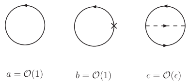
The calculation of the thermodynamic potential with non-zero is very similar to the calculation of Ref. Nishida:2006br . The main difference is that the dependent pieces get contribution from momenta in a window Liu:2002gi ; Bedaque:2003hi . In particular, the first one-loop diagram in Fig. 1 gives a contribution to the effective potential. The second diagram is also . However, the contribution is since the diagram is proportional to an insertion of and there is no enhancement from the finite volume loop-integral for momenta . The two-loop diagram is due to the factors of from the vertices.
The first one-loop diagram from Fig. 1 gives:
| (12) |
We divide the free energy by factors of to look at dimensionless quantities for convenience. Without the loss of any generality, we choose . Then,
| (13) | ||||
with . The contribution from the second one-loop diagram in Fig. 1 gives
| (14) | ||||
where . Thus the leading order effective potential is
| (15) |
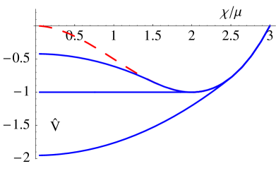
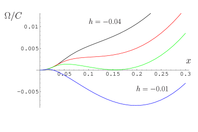
In Fig. 2, we plot the leading order effective potential as a function of for various values of . For , the ground state is a superfluid and the potential is minimized by . At , for all . This is qualitatively different from weak coupling BCS results where the normal and BCS phases are separated by a potential barrier. At leading order in the expansion the superfluid phase is stable all the way up to , compared to the weak coupling BCS result . In addition to that, there is no unstable gapless Sarma phase sarma ; Liu:2002gi ; Bedaque:2003hi ; Wu:2003 for any value of , while BCS calculations predict the presence of a Sarma phase for .
To understand the nature of the transition from superfluid phase to normal phase better, it is necessary to consider the next-to-leading order corrections. A priori it seems unlikely that the “flatness” of the potential for at the critical will be maintained at higher orders in the expansion. The calculation can be simplified by expanding around the leading order value at the critical point, .
The first one-loop diagram gives
| (16) | ||||
is the Euler-Mascheroni constant. The factors of are understood to be expanded to the appropriate order in . The contribution from the last term was already calculated in Eq. (13). The can be calculated analytically but the expression is not very illuminating and we will not write it explicitly.
At next-to-leading order the contribution from the second one-loop diagram in Fig. 1 is
| (17) | ||||
where we have used . The two-loop contribution from Fig. 1 is
| (18) | ||||
where
| (19) | ||||
is the independent piece and
| (20) | ||||
are the corrections. We have defined the functions
| (21) | ||||
Numerical evaluation gives . The contribution from the two-loop diagram is . Therefore we can use in the integrals , at this order of the calculation.
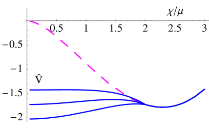
At next-to-leading order in the -expansion, the effective potential is
| (22) |
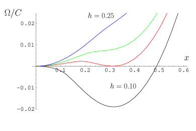
where we use . Results are plotted in Fig. 3 for various values of . The next-to-leading order result is qualitatively similar to weak coupling BCS theory with a stable and unstable superfluid phase. The stable superfluid phase is at Nishida:2006br
| (23) |
The critical chemical potential when the normal and stable superfluid phase are in equilibrium can be determined analytically by equating the corresponding pressures:
| (24) |
This is further simplified because . We find
| (25) | ||||
IV Fermion dispersion relation
The fermion dispersion relation is determined by the pole in the fermion Nambu-Gor’kov propagator. From the inverse propagator at leading order, we get:
| (26) |
which gives . At leading order in the -expansion, the quasiparticle energy has a minimum at with a gap :
| (27) |
The gap decreases linearly with the asymmetry and vanishes at the critical value , where the gapless modes are the ones associated with the normal phase.
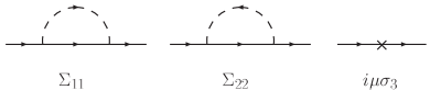
At next-to-leading order, the fermion propagator gets a contribution from the self energy diagrams shown in Fig. 4. The condition for finding the pole in the fermion propagator now reads:
| (28) |
The self-energy contribution is diagonal in the Nambu-Gor’kov space and we find Nishida:2006br :
| (29) | ||||
Close to the minimum of the dispersion relation, we only need to use the leading order values , to evaluate Nishida:2006br . We write . Solving Eq. (28) gives
| (30) | ||||
The contribution from to the dispersion relation at has been calculated before Nishida:2006br . The dependence comes from momentum integrals that involve factors of . Previously in Eq. (24) we found that . Thus for , where the superfluid phase is thermodynamically stable, is actually independent. Therefore, we get
| (31) | ||||
We notice that decreases linearly with even at next-to-leading order. At the critical , the gap is
| (32) |
where we have set . Thus, at this order of the calculation there are no gapless superfluid modes for .
V Stability of the homogeneous phase
We observed that there are no gapless fermion modes at . Nevertheless, given the size of next-to-leading order corrections to and the presence of gapless or almost gapless fermions can certainly not be excluded. Moreover, gapless modes might exist near the unitarity limit at finite scattering lengths. Gapless fermion modes in BCS-type superfluids cause instabilities of the homogeneous superfluid phase, see Wu:2003 ; Huang:2004bg ; Son:2005qx ; Schafer:2005ym ; Kryjevski:2005qq ; Gerhold:2006dt . The dispersion relation Eq. (30) is BCS-like, and we therefore investigate the stability of the homogeneous phase with regard to the formation of a non-zero Goldstone boson current . We note that the dispersion relation is only weakly BCS-like, whereas . As a result any current that is formed is small, and we can neglect terms of higher order in , or inhomogeneities in the absolute magnitude of . The effective potential for is
| (33) |
where is the mass density and is the dispersion relation in the presence of a non-zero current. At leading order it is sufficient to compute the integral Eq. (33) in dimensions. A rough analytical estimate can be obtained by approximating the measure of the angular integration . Introducing the scaling variables
| (34) | ||||
with , and we can write the effective potential as Son:2005qx
| (35) | ||||
where
| (36) |
The functional has non-trivial minima in the range . This means that there is a range of values for in which the ground state support a non-zero supercurrent. The size of this window is parametrically small, , and so is the magnitude of the current, . Using the leading order results for and the fermion dispersion relation we get and . Numerical results for the complete energy functional in are shown in Fig. 5. The result is qualitatively very similar to the approximate solution, but the supercurrent window shrinks by about a factor 3. We get and .
VI Conclusions
We used an expansion around spatial dimension to study the phase structure of a cold polarized Fermi gas at infinite scattering length. At next-to-leading order we find a single first order phase transition from a superfluid phase to a fully polarized normal Fermi liquid. The critical chemical potential is . We also find an unstable gapless Sarma phase. We observe that corrections are sizable, and the presence of gapless superfluid phase cannot be excluded. We show that a gapless superfluid is unstable with respect to the formation of a supercurrent. Recent experiments Zwierlein:2006 indicate the existence of at least one intermediate phase between the superfluid and fully polarized normal state. This suggests that a gapless superfluid phase or partially polarized normal phase is stabilized by finite temperature effects, finite size effects, or higher order corrections in the expansion.
VII Note added
Independently of this work Nishida and Son studied the phase diagram of a polarized Fermi liquid Nishida:2006eu . Where the two investigations overlap, they agree. Since these results appeared Arnold et al. computed the NNLO contribution to the ground state energy of an unpolarized Fermi liquid Arnold:2006fr . The NNLO correction turns out to be large and destroys the apparent convergence and nice agreement with Green Function Monte Carlo calculations observed at NLO. This is maybe not entirely surprising, the naive expansion of the critical exponents in the Ising model also shows poor convergence properties at higher orders. The result of Arnold et al. implies that beyond NLO the expansion has to be improved by combining the expansion with information from the expansion, and by using Pade approximants or similar methods.
Acknowledgements.
This work was supported in parts by the US Department of Energy grants DE-FG02-03ER41260, DE-FG02-87ER40365 and by the National Science Foundation grant PHY-0244822 .References
- (1) M. W. Zwierlein, A. Schirotzek, C. H. Schunck and W. Ketterle, Science 311, 492 (2006).
- (2) G. B. Partridge, W. Li, Y. Kamar, R. I.and Liao and R. G. Hulet, Science 311, 503 (2006).
- (3) M. W. Zwierlein, A. Schirotzek, C. H. Schunck and W. Ketterle, cond-mat/0605258.
- (4) Z. Nussinov and S. Nussinov, cond-mat/0410597.
- (5) Y. Nishida and D. T. Son, cond-mat/0604500.
- (6) J. Carlson, S.-Y. Chang, V. R. Pandharipande and K. E. Schmidt, Phys. Rev. Lett. 91, 050401 (2003).
- (7) S. Y. Chang, V. R. Pandharipande, J. Carlson and K. E. Schmidt, Phys. Rev. A 70, 043602 (2004).
- (8) G. E. Astrakharchik, J. Boronat, J. Casulleras and S. Giorgini, Phys. Rev. Lett. 93, 200404 (2004).
- (9) J. Carlson and S. Reddy, Phys. Rev. Lett. 95, 060401 (2005).
- (10) A. Bulgac, J. E. Drut and P. Magierski, cond-mat/0505374.
- (11) E. Burovski, N. Prokof’ev, B. Svistunov and M. Troyer, Phys. Rev. Lett. 96, 160402 (2006).
- (12) D. Lee, Phys. Rev. B73, 115112 (2006).
- (13) G. Sarma, Phys. Chem. Solid 24, 1029 (1963).
- (14) A. I. Larkin and Y. N. Ovchinikov, Zh. Eksp. Theor. Fiz. 47, 1136 (1964).
- (15) P. Fulde and A. Ferrell, Phys. Rev. A 550, 145 (1964).
- (16) G. Rupak, nucl-th/0605074.
- (17) W. V. Liu and F. Wilczek, Phys. Rev. Lett. 90, 047002 (2003).
- (18) P. F. Bedaque, H. Caldas and G. Rupak, Phys. Rev. Lett. 91, 247002 (2003).
- (19) S.-T. Wu and S. Yip, Phys. Rev. A 67, 053603 (2003) .
- (20) M. Huang and I. A. Shovkovy, Phys. Rev. D 70, 051501 (2004).
- (21) D. T. Son and M. A. Stephanov, Phys. Rev. A 74, 013614 (2006).
- (22) T. Schafer, Phys. Rev. Lett. 96, 012305 (2006) .
- (23) A. Kryjevski, hep-ph/0508180.
- (24) A. Gerhold and T. Schäfer, Phys. Rev. D 73, 125022 (2006) .
- (25) Y. Nishida and D. T. Son, cond-mat/0607835.
- (26) P. Arnold, J. E. Drut and D. T. Son, cond-mat/0608477.