Correlations in a BEC Collision: First-Principles Quantum Dynamics with 150 000 Atoms

Abstract

The quantum dynamics of colliding Bose-Einstein condensates with 150 000 atoms are simulated directly from the Hamiltonian using the stochastic positive-P method. Two-body correlations between the scattered atoms and their velocity distribution are found for experimentally accessible parameters. Hanbury Brown–Twiss or thermal-like correlations are seen for copropagating atoms, while number correlations for counterpropagating atoms are even stronger than thermal correlations at short times. The coherent phase grains grow in size as the collision progresses with the onset of growth coinciding with the beginning of stimulated scattering. The method is versatile and usable for a range of cold atom systems.

The prediction of many-body quantum dynamics is a long term goal of investigation in a variety of scientific fields ranging from physics to chemistry, biology and computation theory. It is a pivotal problem for interacting systems, but challenging because of the complexity of a full description of a quantum system, in which the number of basis states grows exponentially with the number of particles. Experiments with Bose-Einstein condensates of ultra-cold atoms give excellent examples of phenomena that are not well described by standard approximations such as the Gross-Pitaevskii (GP) equation. This equation treats the macroscopically occupied wavefunction, but neglects atomic correlations and fluctuationsDalfovo which are especially prominent in strongly interacting or dimensionally reduced gases, and in condensate collisions. In the latter case, the GP equation fails because the scattering initially occurs spontaneously into unoccupied modes, which are ignored by a macroscopic wavefunction approach. Later, the scattering becomes Bose-enhanced, and a coherent, non-perturbative treatment of the scattered modes is essential.

Treatments of BEC collisions have included a slowly-varying envelope approximation (SVEA) which estimates the scattering cross-sectionsvea , perturbation theoryZin ; Bach , and the semi-classical truncated Wigner methodNorrie12 . The last method is nonperturbative, works well in one dimensionDH93 , and appears to treat both the initial spontaneous scattering and the later Bose enhancement. However, we will show that it gives strongly incorrect results in 3D at large momentum cutoff, because the equations of motion are truncated. Hence, there is a strong incentive to develop a quantitative, first-principles method for these cases.

This Letter also has a broader focus than just BEC. While path-integral Monte Carlo methods are now very successful for calculating equilibrium properties, quantum dynamics is not amenable to these techniques because of the very rapid dephasing between different pathsMonteCarlo . Phase-space distribution methods (such as the Glauber-SudarshanGSp , positive-Ppp , stochastic wavefunctionCarusotto , gauge-PUQbt ) do not suffer from this problem, and yet the scaling is still is only linear in the system size. They have been applied successfully to cold atom quantum dynamics in increasingly large systems, including simulation of evaporative cooling to form a BECCorney , spin squeezing and formation of two-component BECsMolmer , correlation dynamics in a uniform gasdynamix1 , the quantum evolution of Avogadro’s number of interacting atomsUQprl , the dynamics of atoms in a 1D trapCarusotto , and molecular down-conversionSavage .

Here we demonstrate the maturity and ready-to-use nature of the original positive P method for truly macroscopic systems. We simulate an average of 150 000 atoms, requiring $M=1.08\times 10^{6}$ momentum modes. Since each of $M$ modes can have up to about $N$ atoms , the full Hilbert space contains at least $D\approx M^{N}\approx 10^{1\,000\,000}$ orthogonal quantum states (or $D\approx 10^{200\,000}$ if fixed total atom number is assumed). This is one of the largest Hilbert spaces ever treated in a first principles quantum dynamical simulation — made possible by probabilistic sampling rather than brute-force diagonalization.

The use of such a first principles, yet stochastic, simulation confers several advantages in comparison with approximate methods. Firstly, all uncertainty in the results is confined to random statistical fluctuations, with no systematic bias. This uncertainty can be reduced by averaging over more stochastic realizations, and even more importantly, can be reliably estimated from their spread. Secondly, these methods lead to relatively simple equations of motion, which are easily adapted to realistic modeling of trap potentials and local losses.

We consider the collision of two pure ²³Na BECs, with a similar design to a recent experiment at MITVogels . A $1.5\times 10^{5}$ atom condensate is prepared in a cigar-shaped magnetic trap with frequencies 20 Hz axially and 80 Hz radially. A brief Bragg laser pulse coherently imparts a velocity of ${2{\rm v_{Q}}}=19.64$ mm/s to half of the atoms, much greater than the sound velocity of $3.1$ mm/s. At this point the trap is turned off so that the wavepackets collide freely. In a center-of-mass frame, atoms are scattered preferentially into a spherical shell in momentum space with mean velocities ${\rm v_{s}}\approx{\rm v_{Q}}$. As the density of atoms in this shell builds up, Bose-enhancement of scattering into it is expected to begin. Of particular interest are the distribution of scattered atom velocities, and correlations between those atoms, which were recently shown to be experimentally measurableJinBlochAspect .

In present BEC experiments, the system can be described to a high accuracy by the local interaction HamiltonianLeggett :

$$\widehat{H}=\int\,\left[\frac{\hbar^{2}}{2m}\nabla\widehat{\Psi}^{\dagger}\nabla\widehat{\Psi}+\frac{g}{2}\widehat{\Psi}^{\dagger 2}\widehat{\Psi}^{2}\right]\,d\,^{3}\vec{x}\,.$$ (1)

The operator $\widehat{\Psi}^{\dagger}(\vec{x})$ creates a bosonic atom at position $\vec{x}=({\rm x,y,z})$ and obeys commutation relations $[\widehat{\Psi}(\vec{x}),\widehat{\Psi}^{\dagger}(\vec{y})]=\widetilde{\delta}\,^{(3)}(\vec{x}-\vec{y})$, with $\widetilde{\delta}$ a delta-function tempered by a momentum cutoff $\vec{k}_{{\rm max}}$. The coupling constant $g$ depends on the s-wave scattering length $a$ ($2.75$nm in the case of ²³Na), and for $\vec{k}_{{\rm max}}\ll 1/a$ one finds that $g=4\pi\hbar^{2}a/m$.

To calculate time-evolution, we employ the positive P representationpp ; dynamix1 because it preserves the full quantum dynamics. This approach utilizes the completeness of the coherent-state basisGSp . The density matrix $\widehat{\rho}$ is expanded as a positive distribution $P$ over off-diagonal coherent-state projectorspp , thus preserving quantum correlations: $\widehat{\rho}=\int P(\vec{\alpha},\vec{\beta})\ d^{2M}\,\vec{\alpha}\,d^{2M}\vec{\beta}\ \left|\vec{\alpha}\right\rangle\langle\vec{\beta}^{*}|/[\langle\vec{\beta}^{*}\left|\vec{\alpha}\right\rangle]$. Here $\widehat{\Psi}(\vec{x})=\sqrt{1/V}\sum_{\vec{k}}e^{-i\vec{k}\cdot\vec{x}}a_{\vec{k}}\,$ for momentum-mode operators $a_{\vec{k}}$ in a volume $V$. The coherent state $\left|\vec{\alpha}\right\rangle=\otimes_{\vec{k}}\left|\alpha_{\vec{k}}\right\rangle$ is a joint eigenstate of each $a_{\vec{k}}$, with complex eigenvalue $\alpha_{\vec{k}}$GSp . When used to expand the master equation $i\hbar\partial\widehat{\rho}/\partial t=[\widehat{H},\widehat{\rho}\,]$ dynamix1 , this leads to a Fokker-Planck or diffusion equation in the probability $P$, which is equivalent to solving an ensemble of stochastic equations for the sampled variables $\vec{\alpha}$ and $\vec{\beta}$. The equations are simplified on discrete Fourier transforming to a conjugate spatial lattice $\vec{x}$, where $\alpha_{\vec{x}}=\sum_{\vec{k}}\alpha_{\vec{k}}\exp(i\vec{k}\cdot\vec{x})/\sqrt{M}$:

$$i\hbar\frac{d\alpha_{\vec{x}}}{dt} = \left[-\frac{\hbar^{2}}{2m}\nabla^{2}+\frac{g}{\Delta V}\,\alpha_{\vec{x}}\beta_{\vec{x}}+\sqrt{i\hbar g}\ \xi_{\vec{x}}\right]\alpha_{\vec{x}}$$ (2)

$$-i\hbar\frac{d\beta_{\vec{x}}}{dt} = \left[-\frac{\hbar^{2}}{2m}\nabla^{2}+\frac{g}{\Delta V}\,\alpha_{\vec{x}}\beta_{\vec{x}}+\sqrt{-i\hbar g}\ \widetilde{\xi}_{\vec{x}}\right]\beta_{\vec{x}}.$$

Here $\nabla^{2}\alpha_{\vec{x}}$ is the discretized analogue of $\nabla^{2}\alpha(\vec{x})$ for a field, and $\xi_{\vec{x}}$ and $\widetilde{\xi}_{\vec{x}}$ are real Gaussian noises, independent at each time step (of length $\Delta t$) and lattice point, with standard deviations $1/\sqrt{\Delta V\Delta t}$, where $\Delta V=V/M$ .

There is an equivalence between statistical averages of moments of $\alpha_{\vec{k}}$ and $\beta_{\vec{k}}$, and corresponding normally-ordered expectation values of operators $a_{\vec{k}},{\,\,a}_{\vec{k}}^{\dagger}$. As the number of trajectories, $S$, grows towards $\infty$, the correspondence becomes exact. These stochastic equations are just the mean-field GP equations in a doubled phase-space, plus noise terms. Remarkably, these modifications incorporate all effects beyond the GP equation, provided certain phase-space boundary conditions are metUQbt ; dynamix2 .

Uncertainty in the observables is estimated by binning trajectories, then calculating the observable predictions from each bin, and using the central limit theorem to estimate the standard deviation in the final mean of bin means. Lattice spacings $\Delta t$ and $\Delta\vec{x}$ are chosen by reducing them until no further change is seen. In the figures, results are presented in terms of velocity space, $\vec{v}=\hbar\vec{k}/m$, the Fourier transformed field $\widehat{\Psi}(\vec{v}),$ and the velocity space density $\rho(\vec{v})=\langle\widehat{\Psi}^{\dagger}(\vec{v})\widehat{\Psi}(\vec{v})\rangle$.

Following earlier proceduresDC , we discretize onto a $M=432\times 50\times 50$ lattice with $k_{{\rm x,max}}=1.4\times 10^{7}$/m and $k_{{\rm y,z,max}}=6.2\times 10^{6}$/m. We begin the simulation in the center-of-mass frame at the moment the lasers and trap are turned off ($t=0$). The $k_{{\rm max}}$ and lattice size are chosen large enough to encompass all relevant phenomena but small enough that the spacing ($\pi/k_{{\rm max}}$) is much larger than $a$. The initial wavefunction is modelled as the GP solution of the trapped $t<0$ condensate, but modulated with a factor $\left[e^{ik_{{\rm Q}}{\rm x}}+e^{-ik_{{\rm Q}}{\rm x}}\right]/\sqrt{2}$ which imparts initial velocities ${\rm v_{x}}={\rm\pm v_{Q}}=\pm\hbar k_{{\rm Q}}/m$ in the ${\rm x}$ direction. For computational reasons, the mean number of atoms in the system is $1.5\times 10^{5}$ here, compared to $\approx 3\times 10^{7}$ in the MIT experimentVogels . As in other recent treatmentsNorrie12 , we ignore thermal atoms and initial quantum depletion, for simplicity. For our parameters, 10% thermal component will occur at $\approx 0.38T_{c}$Dalfovo , giving a $\approx 1\%$ quantum depletion of the ground state in the center of the cloudDepletion . These small corrections can be included in the initial stateRuostekoski .

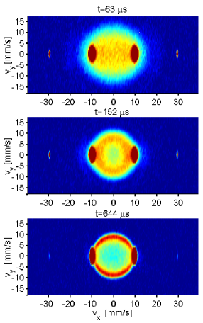
Figure 1: Evolution of velocity distribution. The distribution $\rho({\rm{v_{x}},{\rm{v_{y}})}}$ has been integrated over one transverse dimension ${\rm z}$. Color from blue to red indicates increasing density (its range varies between panels). $S=2048$ trajectories.

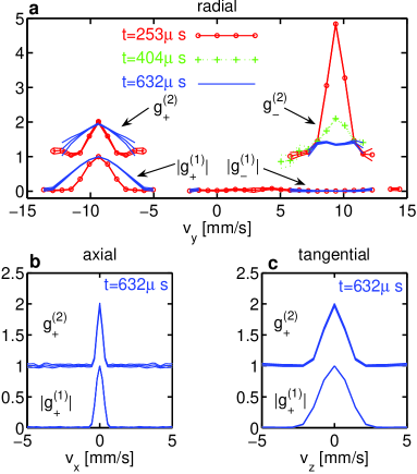
Figure 2: Correlations between scattered atoms. All are between scattered atoms at a maximum density point in the shell (with velocity $\vec{v}_{0}=(0,-9.37,0)$ mm/s relative to the COM) and those with a shifted velocity $\vec{v}$, where: a: $\vec{v}=(0,{\rm v_{y}},0)$, b: $\vec{v}=({\rm v_{x}},0,0)$, and c: $\vec{v}={\rm(0,0,{\rm{v_{z}})}}$. To reduce statistical noise, averages $g_{\pm}^{(n)}=\frac{1}{V_{0}}\int g^{(n)}(\vec{v}_{0}+\vec{\delta v},\vec{v}\pm\vec{\delta v})\,d^{2}\vec{\delta v}$, over a volume $V_{0}$ in velocity space are plottedvol . Triple lines are $1\sigma$ errors.

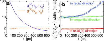
Figure 3: Evolution of correlations between scattered atoms. Parameters and $\vec{v}_{0}$ as in Fig. 2. b: The Full-width half-maximum (FWHM) width of $|g_{\pm}^{(1)}|$ in velocity space.

Figure 1 shows the formation of the scattered atom shell. Careful inspection shows that the mean scattered atom speed ${\rm v_{s}}$ is less than the wavepacket speed ${\rm|v_{Q}|}$, as noted in Bach . We also see weak scattering between two atoms from a wavepacket at $\pm{\rm v_{Q}}$ to one atom at $\pm 3{\rm{v_{Q}}}$ and one at $\mp{\rm{v_{Q}}}$.

Ranged two-body correlations give insight into typical small-scale behaviour during a single experimental run. The first-order correlation function $g^{(1)}(\vec{v}_{1},\vec{v}_{2})=\langle\widehat{\Psi}^{\dagger}(\vec{v}_{1})\widehat{\Psi}(\vec{v}_{2})\rangle/\sqrt{\rho(\vec{v}_{1})\,\rho(\vec{v}_{2})}$, describes coherence between particles with velocity $\vec{v}_{1}$ and $\vec{v}_{2}$. The second-order (number) correlation function $g^{(2)}(\vec{v}_{1},\vec{v}_{2})=\langle\widehat{\Psi}^{\dagger}(\vec{v}_{1})\widehat{\Psi}^{\dagger}(\vec{v}_{2})\widehat{\Psi}(\vec{v}_{1})\widehat{\Psi}(\vec{v}_{2})\rangle/\rho(\vec{v}_{1})\,\rho(\vec{v}_{2})$ gives the average shape and size of “lumps” in the velocity distribution.

The dynamics of the correlations among scattered atoms are shown in Figs. 2 and 3. Locally the atoms are thermally bunched with $g^{(2)}(\vec{v},\vec{v})\approx 2$ in a “Hanbury Brown–Twiss” manner (Fig. 2). This behaviour has been confirmed qualitatively in a similar recent He^∗ experimentWestbrook . The local region over which coherence is strong, dubbed a “phase grain” by Norrie et alNorrie12 , is described by $|g^{(1)}|$. It closely matches the condensate wavepackets’ $\rho(\vec{v})$ in size, and is wider than $g^{(2)}$ by $\approx\sqrt{2}$ (Fig. 2). We find that the orientation of these phase grains is constant throughout the whole spherical shell. Interestingly, after $t\approx 200\,\mu$s, the phase grains expand significantly in the radial direction (relative to COM) (Figs. 2a and 3b). This onset of growth coincides with the beginning of Bose stimulated scattering (see below and Fig. 4a, circles).

Atoms with velocities $\vec{v}$ and $-\vec{v}$ on opposite sides of the spherical shell are not coherent ($|g^{(1)}|\approx 0$), but are correlated in number (Fig. 2a). Initially, correlations are extreme: $g^{(2)}(k,-k)\gg 2$. This is analogous to a two-mode mixed state $p\,|1,1\rangle\langle 1,1|+(1-p)\,|0,0\rangle\langle 0,0|$ with a small probability $p\,$ of single atoms in both modes and otherwise vacuum. There $g^{(2)}=1/p$. At longer times, $g^{(2)}$ is seen to decay in Fig. 3a, although it is still much greater than the thermal value of two for $t\gtrsim 200\mu$s when the phase grain contains several atoms. To measure short time velocity correlations, one might try to preserve them by suddenly switching off the atomic interactions using a Feshbach resonance during the collision. After expansion, they would develop into position correlationsJinBlochAspect .

Some previous correlation estimates are in qualitative agreement: For longer times, $g^{(2)}(\vec{v},\vec{v})=2$, as well as $g^{(2)}(\vec{v},-\vec{v})\approx 2$ and $g^{(1)}(\vec{v},-\vec{v})\approx 0$ were predictedZin . Truncated Wigner calculationsNorrie12 saw the presence of phase grains, but their orientation or dynamics were not studied. High initial correlations may have not been seen due to the known poor signal-to-noise ratio in that method.

The scattering rate (Fig. 4a, circles) goes through two distinct phases: The spontaneous regime of constant scattering into almost empty modes is seen for $30\,\mu$s$\,\lesssim t\lesssim 200\,\mu$s, followed by the stimulated (Bose-enhanced) regime for times $t\gtrsim 200\,\mu$s, where there is a decided increase in scattering rate despite a lessening overlap between the colliding wavepackets. We interpret this transition as the onset of Bose enhancement of scattering into the spherical shell around $|\vec{v}|\approx{\rm v_{s}}=9.37$ mm/s. As a rough check, it should begin when the number of particles in a locally coherent region (“phase grain”) approaches one. Using the widths of $g^{(1)}$ from Fig. 3b, and the calculated density at $|\vec{v}|={\rm v_{s}}$ one finds $\approx 0.9$ atoms per phase grain at $200\,\mu$s.

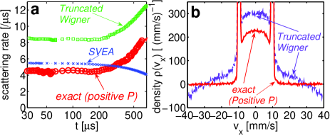
Figure 4: Comparison of exact and approximate methods. Panel a: Rate of scattering out of coherent wavepackets. Obtained by counting atoms outside of spheroidal regions covering the coherent wavepackets centered at $\pm{\rm v_{Q}}$ and $\pm 3{\rm v_{Q}}$. Panel b: Distribution of axial (x) velocity of scattered atoms at $t=657\mu$s; In both panels: $S=2048$ (Pos. P), $S=672$ (Wigner).

A comparison to approximate methods used previously is instructive. Fig. 4 shows our total predicted scattering rate and the distribution of axial (x) velocities, compared to the approximate truncated Wigner method. The accuracy of that method is very poor with our parameters, even surprisingly so. It adds a halo of false particles (detail in Fig 4b) out to about $\pm 2{\rm v_{Q}}$, while at higher velocities unphysical negative densities are obtained. Since it is a hidden-variable theory it must introduce half a virtual particle per mode in the initial conditions to model vacuum fluctuations, but it does not distinguish them from the “real particles”. Then, virtual particles at velocity $\vec{v}$ are scattered by the condensates at $\approx\pm\vec{v}_{{\rm Q}}$ in the process $\vec{v}\ \&\ \pm\vec{v}_{{\rm Q}}\ \to\ \vec{v}\,^{\prime}\ \&\ (\vec{v}\pm\vec{v}_{{\rm Q}}-\vec{v}\,^{\prime})$. As a result, modes at high velocities become depleted compared to the physical vacuum, while the extracted virtual particles accumulate at lower velocities and take on the appearance of a real density, as was also discussed previouslySinatra .

For any single momentum mode this effect is small, but it becomes very significant when a large number of modes are calculated. A relatively higher momentum cutoff will increase the error, as the fraction of virtual particles increases (or vice-versaNorrie12 ). This indicates a generic ultra-violet divergence of the error with the truncated Wigner method.

The main limitation of the positive-P method is the growth of sampling uncertainty with time. It eventually reaches a size where it is no longer practical to produce enough trajectories for useful precision. In our case useful results are obtained for $t\lesssim 660\,\mu$s. This useful time range depends on several factors, with coarser lattices, weaker interactions, or smaller density all extending itdynamix1 . Significant extensions appear achievable by tailoring appropriate stochastic gaugesdynamix2 ; UQbt or basis sets to particular systems.

In conclusion, we have simulated the quantum dynamics of macroscopic interacting Bose gases from first-principles, obtaining momentum space densities and ranged correlation functions for atoms scattered during the collision of two BECs. Previous approximate calculations were partly verified, while a variety of new phenomena are also predicted, including the growth of phase grains in the radial momentum direction, and strong correlations at short times between scattered atom pairs. The truncated Wigner method was confirmed strongly incorrect in regimes where the number of condensed atoms per lattice site is less than one.

This demonstrates that phase-space methods are a tool that is ready-to-use for first principles calculations for experimentally realizable systems. Similar calculations appear feasible for a broad range of cold atom systems (including fermionsCorneyDrummond ). A range of other phenomena that are difficult to describe quantitatively with approximate methods (e.g. macroscopic EPR and entanglementMacro ) may be accessible with this approach.

- (1) F. Dalfovo et al., Rev. Mod. Phys. 71, 463 (1999).
- (2) Y. B. Band et al., Phys. Rev. Lett. 84, 5462 (2000); T. Köhler, K. Burnett, Phys. Rev. A 65, 033601 (2002).
- (3) P. Ziń et al., Phys. Rev. Lett. 94, 200401 (2005).
- (4) R. Bach, M. Trippenbach, K. Rzażewski, Phys. Rev. A 65, 063605 (2002).
- (5) A. A. Norrie, R. J. Ballagh, C. W. Gardiner, Phys. Rev. Lett. 94, 040401 (2005); eprint cond-mat/0602061.
- (6) P. D. Drummond, A. D. Hardman, Europhys. Lett. 21, 279 (1993).
- (7) E. L. Pollock, D. M. Ceperley, Phys. Rev. B 30, 2555 (1984).
- (8) R. J. Glauber, Phys. Rev. 131, 2766 (1963); E. C. G. Sudarshan, Phys. Rev. Lett. 10, 277 (1963).
- (9) P. D. Drummond, C. W. Gardiner, J. Phys. A: Math. Gen. 13, 2353 (1980).
- (10) I. Carusotto, Y. Castin, J. Dalibard, Phys. Rev. A 63, 023606 (2001).
- (11) P. Deuar, P. D. Drummond, Phys. Rev. A 66, 033812 (2002); P. D. Drummond, P. Deuar, J. Opt. B: Quantum Semiclass. Opt. 5, S281 (2003).
- (12) P. D. Drummond, J. F. Corney, Phys. Rev. A 60, R2661 (1999).
- (13) U. V. Poulsen, K. Molmer, Phys. Rev. A 63, 023604 (2001); 64, 013616 (2001).
- (14) P. Deuar, P. D. Drummond, J. Phys. A 39, 1163 (2006).
- (15) M. R. Dowling et al., Phys. Rev. Lett. 94, 130401 (2005).
- (16) C.M. Savage, P. E. Schwenn, K. V. Kheruntsyan, Phys. Rev. A 74, 033620 (2006).
- (17) J. M. Vogels, K. Xu, W. Ketterle, Phys. Rev. Lett. 89, 020401 (2002).
- (18) M. Greiner et al., Phys. Rev. Lett. 94, 110401 (2005); S. Folling et al., Nature 434, 481 (2005); M. Schellekens et al., Science 310, 648 (2005).
- (19) A. J. Leggett, Rev. Mod. Phys. 73, 307 (2001).
- (20) P. Deuar, P. D. Drummond, J. Phys. A 39, 2723 (2006).
- (21) P. D. Drummond and S. J. Carter, J. O. S. A. B4, 1565 (1987).
- (22) K. Sacha, Kondensat Bosego-Einsteina, (Uniwersytet Jagiellonski, Kraków, 2004, ISBN:83-920033-5-7) p. 74.
- (23) L. Isella, J. Ruostekoski, Phys. Rev. A 72, 011601(R) (2005).
- (24) C. I. Westbrook et. al., eprint quant-ph/0609019.
- (25) A. Sinatra, C. Lobo, Y. Castin, J. Phys. B 35, 3599 (2002).
- (26) O. Juillet, Ph. Chomaz, Phys. Rev. Lett. 88, 142503 (2002); J. F. Corney, P. D. Drummond, ibid. 93, 260401 (2004).
- (27) K. V. Kheruntsyan, M. K. Olsen, and P. D. Drummond, Phys. Rev. Lett. 95, 150405 (2005); E. G. Cavalcanti and M. D. Reid, Phys. Rev. Lett. 97, 170405 (2006).
- (28) These are with lying in the volume , which had dimensions mm/s in the x and z directions, respectively, and was chosen small enough that does not vary significantly within it, as evidenced by .