New methods to determine the Hausdorff dimension of vortex loops in the $3DXY$ model

Abstract

The geometric properties of critical fluctuations in the $3DXY$ model are analyzed. The $3DXY$ model is a lattice model describing superfluids. We present a direct evaluation of the Hausdorff dimension $D_{H}$ of the vortex loops which are the critical fluctuations of the $3DXY$ model. We also present analytical arguments for why $\vartheta$ in the scaling relation $\eta_{\phi}+D_{H}=2+\vartheta$ between $D_{H}$ and the anomalous scaling dimension of the corresponding field theory, must be zero.

I Introduction

It has been proposed that a second-order phase transition is characterized by the breakdown of a generalized rigidity associated with a proliferation of defect structures in the order parameter Anderson_book . In the case of extreme type-II superconductors, it has been explicitly demonstrated that the system undergoes a continuous phase transition driven by a proliferation of closed loops of quantized vorticity Tesanovic_blow_out ; Nguyen ; Nguyen_alpha_determination . In particular, it has been demonstrated that the connectivity of the vortex-tangle (the tangle of topological defects of the system), changes dramatically at the critical temperature of the system Nguyen ; Nguyen_alpha_determination . In other words, it is possible to describe the superconducting phase transition in terms of the proliferation of defect structures (viz. vortices and flux lines), which are singular phase fluctuations and determine the critical properties of the theory. Using this argument, it is possible to relate the critical properties of the phase transition to the geometric properties of the loops Hove_Sudbo at the critical point.

The phenomenology of superconductivity usually starts with the Ginzburg Landau (GL) model. The Hamiltonian for this model is

$$H(q,u_{\psi})=m_{\psi}^{2}|\psi|^{2}+\frac{u_{\psi}}{2}|\psi|^{4}+|D_{\mu}\psi|^{2}+\frac{1}{2}\left(\nabla\times\mathbf{A}\right)^{2}.$$ (1)

Here $\psi=|\psi|e^{i\theta}$ is a complex matter field, coupled to a massless gauge field $\mathbf{A}$ through the minimal coupling $D_{\mu}=\partial_{\mu}-iqA_{\mu}$. $m_{\psi}$ is the mass parameter for the $\psi$ field, and $u_{\psi}$ is the self-coupling. This is a rich model which embodies many different aspects of superconductivityMo:2002 , in this paper we will focus on the limit $\kappa\gg 1$ corresponding to extreme type-II superconductors. In this case the gauge field fluctuations can be ignored, and we are left with a neutral $|\psi|^{4}$ theory. For this theory it can be shown that amplitude fluctuations in $\psi$ are innocuousNguyen ; Nguyen_alpha_determination , and only the phase variables must be retained. When the resulting model is defined on a lattice, one obtains the 3DXY model.

The 3DXY model is a model for phase fluctuations, and both the smooth spin wave fluctuations, and the singular transverse fluctuations are accounted for. The transverse phase fluctuations are defined by

$$\nabla\times\nabla\theta(\mathbf{r})=2\pi\mathbf{n}(\mathbf{r})$$ (2)

where $\mathbf{n}(\mathbf{r})$ is the local vorticity. The vortices are the critical fluctuations of the theory, which drive the superfluid density to zero in the neutral case, and the magnetic penetration length to infinity in the charged case. We have performed simulations directly on the phase degrees of freedom, and extracted the vortex content according to Eq. (2), alternatively it is possible to integrate out the spin wave degrees of freedom and retain only the vortex degrees of freedom Peskin . The definition Eq. (2) ensures that $\nabla\times\mathbf{n}=0$ everywhere, hence the vorticity must be in the form of closed loops.

Since the vortex loops are the critical fluctuations of the theory it is natural to formulate a theory expressed in terms of these degrees of freedom. In $d=3$ it is possible to start with the charged theory Eq. (1) in a fixed-amplitude approximation and derivePeskin a field theory for the vortex loops. It turns out that this dual theory is a neutral $|\phi|^{4}$ theory. Hence, the dual of a charged superfluid is a neutral superfluid and vice versa, and furthermore the vortex loops of a neutral (charged) superfluid are described by a field theory isomorphic to a charged (neutral) superfluid. In this paper we will use the convention that $\psi$ represents the original superfluid, and that $\phi$ is the corresponding dual. Then $\phi$ will be the field theory for the vortices of $\psi$.

The description in terms of loops is physically appealing. Firstly, it highlights the physical meaning of the $|\phi|^{4}$ term which, depending on the sign of $u_{\phi}$, represents a steric repulsion (as in the case of type-II superconductors) or a steric attraction for type-I superconductors with a first order transitionMo:2002 . In the case of a neutral superfluid the vortices will interact attractively through a long range interaction mediated by a dual gauge field, this will yield a vortex tangle more dense than a set of random loopsHove_Mo_Sudbo .

A geometric interpretation of the critical point in terms of proliferating geometric objects was given already in 1967 by M. E. Fisher Fisher:1967 . He considered droplets of one phase immersed in a background phase. Close to the critical point the distribution of droplet size was argued to behave as

$$n(s)\propto\frac{1}{s^{\tau}}e^{-s\epsilon},\quad\epsilon\propto|T-T_{c}|^{\frac{1}{\sigma}},$$ (3)

$n(s)$ is the mean number of droplets of “mass” $s$. The behavior of Eq. (3) is governed by two critical exponents $\sigma$ and $\tau$, where the former governs the vanishing tension when approaching the critical point and $\tau$ is related to the entropy of a droplet. These two exponents can be related to the six ordinary critical exponents

$$\alpha =2-\frac{\tau-1}{\sigma} \beta_{\mathsf{G}} =\frac{\tau-2}{\sigma} \delta_{\mathsf{G}} =1+\frac{\tau-1}{d(\tau-2)}$$

$$\eta_{\mathsf{G}} =2+\frac{d(\tau-3)}{\tau-1} \nu =\frac{\tau-1}{d\sigma} \gamma_{\mathsf{G}} =\frac{3-\tau}{\sigma}.$$ (4)

The distribution $n(s)$ Eq. (3) is also used to describe the cluster density close to the critical point in percolation, and the relations Eq. (4) can be easily derived from that context as wellStauffer:1991:book . The exponents in Eq. (4) have an index $\mathsf{G}$ to emphasize their geometric origin. These exponents will in general not agree with those of the underlying model. The Fortuin-Kasteleyn clustersFortuin:1972 of the Q-state Potts model is a special case where the exponents derived from $\tau$ and $\sigma$ agree with those of the ordinary Potts model, i.e. $\beta_{\mathsf{G}}=\beta,\gamma_{\mathsf{G}}=\gamma,\ldots$. The vortices of the 3DXY model, which we study in this paper, constitute another special case, here the exponents derived from $\tau$ and $\sigma$ agree with the dual of the initial theory. Since the dual of a neutral superfluid is a charged superfluid, the study of the vortices in the 3DXY model can actually be used to glean knowledge of the critical properties of a charged superfluid. In particular, this can be used to relate the anomalous scaling dimension of the Ginzburg Landau theory, $\eta_{\phi}$ to the fractal dimension of the vortex loops in the 3DXY model.

The paper is organized as follows. In section II we derive the relation between the fractal Hausdorff dimension $D_{H}$ of the loops and the anomalous dimension of the dual condensate, $\eta_{\phi}$. Sections III and IV are devoted to presenting our results from Monte Carlo simulations. As a benchmark, we determine the fractal dimension of percolation clusters in section III, and in section IV we determine the fractal dimension of the vortex loops of the 3DXY model. Finally, in Section V we discuss our results.

II Relation between the Hausdorff and the anomalous dimensions

The anomalous dimension $\eta_{\phi}$ of the $\phi$ field is defined as the critical exponent of the correlation function as follows

$$G(\textbf{x},\textbf{y})=\langle\phi(\textbf{x})\phi^{{\dagger}}(\textbf{y})\rangle.$$ (5)

This correlation function has the standard form at large distances at the critical point, namely

$$G(x)\sim 1/x^{d-2+\eta_{\phi}}\qquad x\to\infty,$$ (6)

where $d$ the spatial dimension of the system. Particle-field duality dictates that this correlation function has a geometric interpretation, yielding the probability amplitude of finding any particle path connecting x and y. In the present work, the particle trajectories correspond to vortex loops which can be deduced from the phase distribution of the matter field. It is essential that any vortex path connecting two points x and y must be part of a closed vortex loop, since only closed vortex loops provide the vortex paths in this system. To highlight the important properties of the probability amplitude $P(\textbf{x},\textbf{y},N)$ of connecting two points x and y by a continuous vortex path, we start by focusing on the properties of the vortex loops.

It is known that for random loops in a lattice, the number of steps $N$, defined as the number of occupied links, and the average distance $R_{F}=\sqrt{\Delta_{x}^{2}+\Delta_{y}^{2}+\Delta_{z}^{2}}$, where $\Delta_{i}$ are the coordinate variations of the trajectories, are related by

$$R_{F}\sim N^{1/D_{H}}\qquad N\rightarrow\infty$$ (7)

where $D_{H}$ is the Hausdorff dimension def:fractal_dimension .
Since these vortex are the critical fluctuations of the theory their average size $R_{F}$ is related to the correlation length $\xi$ of the field $\phi$ so that we can set $\xi\sim R_{F}$

$$\xi\sim N^{1/D_{H}}.$$ (8)

With this we can now relate the correlation function $G(x,y)$ with the Hausdorff dimension $D_{H}$ by taking advantage of the fact that in every second order transition the system is scale invariant at $T=T_{c}$. We can, then, write the following scaling Ansatz for the probability amplitude $P(\textbf{x},\textbf{y},N)$

$$P(x,y,N) \propto P(|r|,N)\propto\frac{1}{\xi^{d}}F\left(\frac{|r|}{\xi}\right)$$ (9)

$$\propto N^{-d/D_{H}}F\left(\frac{|r|}{N^{1/D_{H}}}\right)$$

where $P(x,y,N)$ is the probability of finding a loop of length $N$ connecting the points $x$ and $y$. The probability of coming back to the starting point is generally given by $P(x,x,N)$. For some models like self avoiding walks (SAW) and random walks in $d\geq 3$ this probability is vanishing, and the scaling function $F(z)$ has the limiting behavior

$$\lim z\to F(z)=z^{\vartheta},\qquad\vartheta>0.$$ (10)

In the case of vortex loops, which are closed, we clearly must have $\vartheta=0$. This is discussed in more detail in Appendix A. At the critical point the two-point correlation function $G(r)$, Eq.(5), scales with an anomalous dimension $\eta_{\phi}$. At the same time we know that, by the definition of $P(x,y,N)$ together with Eq.(9):

$$G(x,y)=\sum_{N}P(x,y,N)=\sum_{N}N^{-d/D_{H}}F\left(\frac{|r|}{N^{1/D_{H}}}\right).$$ (11)

If we focus on the long loop regime ($N\gg 1$), we can replace the summation with an integral and obtain

$$G(x,y)\sim\int dn\>n^{-d/D_{H}}F\left(\frac{|x-y|}{n^{1/D_{H}}}\right)=\frac{C}{|x-y|^{d-D_{H}}}.$$ (12)

Therefore, we can relate the anomalous dimension $\eta_{\phi}$ to the fractal dimension of the vortex loops, $D_{H}$, as follows

$$\eta_{\phi}+D_{H}=2.$$ (13)

We can also relate $D_{H}$ and, indirectly $\eta_{\phi}$, to another critical exponent, $\tau$, which is related to the density of loops in the system. From the definition of loop density we have

$$D(N)\propto\frac{1}{N}\sum_{x}P(x,x,N)$$ (14)

here, $P(x,x,N)$ is the probability of finding a closed loop of length $N$ and $D(N)$ is the mean number of loops of length $N$. Near $T_{c}$ the loop distribution will then take the form

$$D(N)\sim N^{-\tau}.$$ (15)

If the system is homogeneous, all the contributions in Eq.(14) are equal. Thus, picking an arbitrary $x$ we find

$$P(x,x,N)\propto\frac{N}{V}D(N)\propto N^{1-\tau}.$$ (16)

Finally, combining Eq.(9), Eq.(16) and Eq.(7) we arrive at the following relations

$$\frac{d}{D_{H}} = \tau-1$$ (17)

$$\eta_{\phi} = 2-D_{H}=2-\frac{d}{\tau-1}.$$ (18)

It can be seen from Eq.(13) and Eq.(18) that the anomalous dimension of the dual condensate can be determined either through the determination of $\tau$ or $D_{H}$, the former being statistically easier to evaluate. However, $\eta_{\phi}$ is quite sensitive to $\tau$ [$\partial\eta_{\phi}/\partial\tau=d/(\tau-1)^{2}\sim 1.5$].

The purpose of the present work is to carry out a direct evaluation of $D_{H}$ which facilitates a check of the scaling law Eq. (17). For this reason, the first part of this study has been devoted to test their validity and the validity of the algorithms used in the case of a percolation transition, since it has been extensively studied in the literature and can be easily implemented.

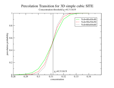
Figure 1: (Color online) Percolation probability of sites as a function of concentration $p$ for a simple 3D cubic system. The concentration at which percolation takes place is given by the common inflection point of the different curves for increasing lattice size.

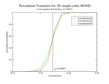
Figure 2: (Color online) Same as Fig.1, but for a bond percolation

Before we start, let us return to the points made above concerning the HT-graph expansion of the partition function and two-point correlation functionsProkof ; Janke . Suppose one were to compare the Hausdorff dimension of physical vortex loops Hove_Sudbo with the Hausdorff dimension of the sort of open ended, self-avoiding walks that one would consider in a HT-graph expansion of the two-point correlation function Prokof . We may compute the loop-distribution function for vortex loops, $D_{\rm{loop}}(N)\sim N^{-\tau_{\rm{loop}}}$, with the distribution of “closed” graphs in self-avoiding walks $D_{\rm{SAW}}(N)\sim N^{-\tau_{\rm{SAW}}}$. A self-avoiding walk of length $N$ is defined as “closed” if one after $N$ steps ends up on a lattice point which is nearest neighbor to the starting point Prokof ; Janke , see also Fig. 1 of Janke . From Fig. 1 in Ref. Janke , it is immediately clear that the stop criterion for defining a “closed” self-avoiding walk, if applied to real physics vortex loops, would mean that one would discard a tail in the distribution function involving large vortex loops. This is so since one could connect the remaining last bridge by an arbitrarily long and complicated vortex path, not just over the shortest link. (In fact, these two point were connected by an arbitrarily long and complicated path, and there is no reason to close the path only by the shortest distance). This would lead to an overestimate for $\tau_{\rm{loop}}$, since removing large loops means that $D(N)$ drops too much as a function of $N$. An overestimate of $\tau$ would lead to an underestimate of $D_{H}$, cf. Eq. (17). In the scaling relation $\eta_{\phi}+D_{H}=2$, it is crucial to compute $D_{H}$ from the real physical vortex loops of the system. If one underestimates $D_{H}$ by for instance considering the fractal Hausdorff dimension of other objects than real physical vortex loops, this might lead one to erroneously conclude that one needs to introduce an additional exponent $\vartheta>0$ and modify the scaling relation to $\eta_{\phi}+D_{H}=2-\vartheta$. While $\vartheta>0$ is needed in the case of self-avoiding walks, this is not so for vortex loops due to the topological constraint ${\bf\nabla}\cdot{\bf n}=0$.

III Results for the percolating systems

Percolation theory is used to describe a variety of natural physical processes where disorder is an essential ingredient. Applications range from spontaneous magnetization of diluted ferromagnets, formation of polymer gels, electrical conductivity of amorphous semiconductors and many othersStauffer:1991:book .

In link (site) percolation the links (sites) of a lattice are occupied independently with probability $p$, and then the resulting clusters of connected links (sites) are analyzed. For small $p$ we will only have small clusters, and the there will be no path connecting the edges of the system. For large $p$ there will be large clusters comparable to the entire system, and the system can sustain a current from edge to edge. The transition from an insulator to metal is a second order (geometric) phase transition at a critical value $p_{c}$.

Figs.1 and 2 show our results for the percolation probability, i.e. the probability that there is at least one cluster spanning the whole system, for sites and bond percolation respectively. We have found $p_{c}=0.311619$ and $p_{c}=0.248627$, respectively. These values agree reasonably well with existing results pc_perc_determination . Clusters have been identified using the Hoshen-Kopelman (HK) HK labeling algorithm and up to $10^{4}$ configurations were considered in the measurements.

We next focus on the calculation of the fractal dimension of percolation clusters at the critical point, and compare with results from the literature D_H_percol_determination . Formally the fractal dimension can be defined from the box counting technique def:fractal_dimension . The fractal object is covered with boxes of linear size $l$, and we count the number of boxes needed for complete coverage. The fractal dimension is inferred from the variation in total number of boxes $N(l)$ with box size $l$ as follows

$$N(l)\propto{\lim_{l\to 0}}\;\;l^{-D_{H}}.$$ (19)

Defining $l$ on a lattice is difficult since the lattice spacing $a$ is a fixed dimensionless constant. Instead, we can relate $l$ to $1/R_{F}$, which is equivalent to considering loops of different size $R_{F}$ as the same loop, but at a different length scale. This relation is unique provided that the different loops can be embedded in a box $\Delta_{x}\Delta_{y}\Delta_{z}$ of the same shape, i.e.

$$\frac{\Delta_{i}}{\Delta_{j}}=C_{ij}\qquad\forall\quad i\neq j\qquad i,j\;\in\;\;[1,3].$$ (20)

where $C_{ij}$ are constants enforcing a constant proportion constraint ($\tt{CPC}$). This implies that loops have to be divided into groups, each one characterized by the actual values of the two independent ratios $C_{ij}$, say $C_{xy}$ and $C_{xz}$, and Eq.(19) applies separately to each group. In the current paper we have only considered cubic boxes with $\Delta_{x}=\Delta_{y}=\Delta_{z}$.

From Eq.(7), it can be seen that there is a relation between the dimension of the cluster (i.e. the number of cells) and its radius (i.e. the dimension of the box containing it). Thus, we first relate the number $N$ of occupied cells by the loops to their length $R_{F}$ using an embedding box of fixed shape $\Delta_{x}=\Delta_{y}=\Delta_{z}$. Although this approach is very close in spirit to the definition Eq. (19) the method fails miserably giving $D_{H}=1.329(8)$, which deviates strongly from the literature results $D_{H}=2.5230$D_H_percol_determination .

The problem, we believe, is that this method (later called $\tt{Method1}$) is affected by two strong restrictions. Firstly, every box must scale in all the three directions in the same way (because of the $\tt{CPC}$), i.e. all the boxes have to be cubes. Secondly, the extraction of the box can be mistaken if the cluster extends beyond the borders of the lattice, so that boxes touching the borders are excluded. For these two reasons the statistics of $N(R_{F})$ in $\tt{Method1}$ is extremely poor, and a correct value of $D_{H}$ cannot be found.

Another way to extract $D_{H}$ is to consider the largest cluster for every configuration, and assume that the box containing this cluster consists of the entire lattice. When the linear size of the lattice is varied this gives the fractal dimension from

$$N^{\ast}\propto L^{D_{H}},$$ (21)

where $N^{\ast}$ is the size of the largest cluster and $L$ is the linear extent of the lattice. Using this approach we have found $D_{H}=2.52$, which is consistent with the value $\tau=2.189$.

Hence, the study of the percolation transition has been useful to first test the simulation and the algorithms used for the extraction of the geometrical properties and, ultimately, it has provided a test of Eq.(17). We can now proceed to the more difficult task of determining the Hausdorff dimension for the ensemble of vortex loops generated by thermal transverse phase fluctuations of the $3DXY$ model.

IV Results for the 3DXY model

The Hamiltonian for the case of a neutral condensate in the London approximation (i.e. neglecting amplitude fluctuations) is given by

$$H(q=0,\theta)=-J\sum_{\langle i,j\rangle}\cos(\theta_{i}-\theta_{j}).$$ (22)

Eqs.(17) and (13) are valid only at the transition point where the system is scale invariant. Therefore the simulations must be restricted to the case $T=T_{c}$.

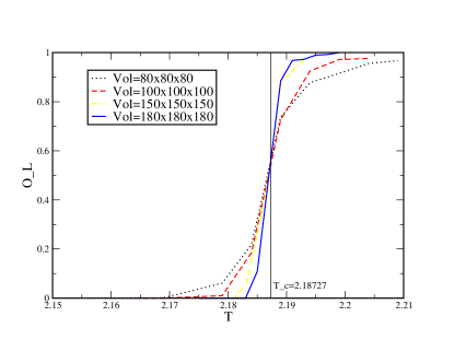
Figure 3: (Color online) Percolation probability $O_{L}$ as function of temperature $T$ for the $3DXY$ model at different lattice sizes. The critical temperature is given by the common inflection point of the different curves for increasing lattice size. The value obtained is $T_{c}=2.18727$

We have used the standard Metropolis algorithms for lattice sizes of $L=80,100,150,180$, all the runs had a hot start and 5000 sweeps were discarded before measurements were made. Vortices are found identifying singularities in the phase configuration according to Eq. (2). The temperature found ($T=2.18727$, cf. Fig.3) is close to, but different from the thermodynamical one, $T_{c}=2.20184$ T_c_3dxy . Variations with the dimension of the system are still present, and it cannot be excluded that in the thermodynamical limit the two values merge together. More extensive simulations along with a finite-size scaling analysis will be necessary to provide this question with a more satisfactory answer.

For the time being, since any $T\geqslant T_{c}$ is better than $T<T_{c}$ to test Eq.(17), all the following simulations will be done at the fixed temperature of $T_{c}=2.20184$. Now that the temperature has been set, $\tau$ and $D_{H}$ can be determined separately and their values compared to the ones available in the literature.

All the simulations were performed on a system of fixed size $L=200$ using up to 40 2Ghz Pentium4. The Monte Carlo runs had a cold start and $10^{4}$ sweeps were discarded for thermalization before taking measurements over $4\cdot 10^{5}$ configurations. The loops in the system are identified with a modified version of the Hoshen-Kopelman algorithm which resolves vortex crossings randomly. The exponent $\tau$ for the loop distribution has been determined earlier as $\tau=2.310(3)$ Nguyen_alpha_determination ; Hove_Sudbo . The results obtained for $\tau$ are shown in Fig.4.

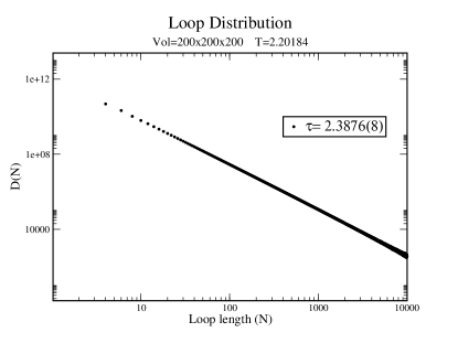
Figure 4: Vortex-loop distribution $D(N)\sim N^{-\tau}$ as a function of perimeter length $N$ at the temperature $T=2.18727$, as explained in the text.

We now turn to the fractal dimension $D_{H}$. The first interesting fact is that the method used to extract the pair (length, box) used in the percolation transition does not work any more, giving unphysical values for $D_{H}$. On the other hand, the more correct method of extracting the exact box containing the loops yields a value in agreement with Eq.(17).

There is also a topological reason for which we can expect to have different statistics for the two systems (and therefore we need to apply two different methods). When extracting the clusters in a percolating system, all connected sites (or bonds) are considered part of the same object, i.e. belonging to the same cluster. In general, this will lead to fewer but larger clusters in the system, this is particularly the case at the transition point, where the cluster tension vanishes. In the case of vortex-loops, on the other hand, two intersecting loops are connected with $50\%$ probability, which directly influences the value of $\tau$ which is smaller in the case of percolation.

IV.1 Method1

We have tested $\tt{Method1}$, and the extracted value of $D_{H}=2.168(6)$ (Fig.5) is in good agreement with the expected one of $D_{H}\simeq 2.162(1)$, as calculated using Eq.(17), and the value of $\tau=2.3876(8)$ previously obtained (Fig.4).

Eq.(7) is assumed to hold only in the limit $N\to\infty$, so that small deviations from linearity are expected for small $N$ where the discrete form of the lattice becomes important. Therefore, in order to reduce these lattice effects, we have varied the lower cutoff on $R_{F}$ systematically. Results are shown in Fig.6, which is characterized by a ‘saturation’ in the long-loop regime. To obtain a reliable value of $D_{H}$ this saturation region has to be reached, but, although this is the case, there are still considerable fluctuations.

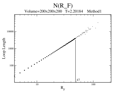
Figure 5: Loop length $N(R_{F})$ as a function of the characteristic size $R_{F}$. The best fit has been performed only on the point between $4\leq R_{F}\leq 47$.

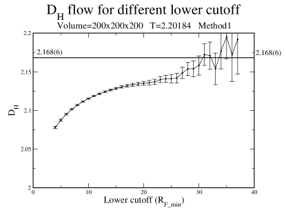
Figure 6: Variation of $D_{H}$ with the lower cutoff. The saturation expected in the continuum limit is present but strongly effected by fluctuations. The finale value of $D_{H}$=2.168(6) is obtained using a weighted fit over the last eight points

For this reason and owing to the results obtained for percolating systems, we have considered two new methods in order to determine values of the Hausdorff dimension $D_{H}$ with better precision. The main limitation in Method1 is the limited statistics, in an attempt to improve on this situation we have devised two additional methods to calculate $D_{H}$. Both methods rely on ‘relaxation’ of the $\tt{CPC}$ constraint.

The strongest statistical limitation on $\tt{Method1}$ is that the loops have to be divided into groups and that only comparison within each group are allowed. The consequence of this restriction can be directly seen in Fig.5, where the longest loop considered has a linear dimension of $\sim 47$, to be compared with the linear dimension of the lattice of $200$. Clearly then, the longest loops present in the lattice (the ones for which Eq.(7) holds) are excluded from the final statistics obtained.

IV.2 Method2

The first of these two new methods ($\tt{Method2}$ below) determines a lower and an upper bound for $R_{F}$. To see how this can be done let us consider a box containing a loop with the condition $\Delta_{x}=\Delta_{y}=\Delta$ and $\Delta_{z}=\Delta+C$ where $C$ is some constant, and $\Delta_{x},\Delta_{y},\Delta_{z}$ the dimensions of the box containing the loop in the three directions. We immediately observe that, since $C$ is constant, there is a violation of the $\tt{CPC}$

$$\frac{\Delta_{z}}{\Delta_{x}}=\frac{\Delta+C}{\Delta}\neq\frac{\Delta^{\prime}+C}{\Delta^{\prime}}=\frac{\Delta^{\prime}_{z}}{\Delta^{\prime}_{x}}.$$ (23)

However, the error is of the order of $C/\Delta$, so in the limit of large boxes ($\Delta\gg C$) this approximation is exact. We can then define the following loop size $R_{F}$ as follows

$$R_{F} = \sqrt{\Delta_{x}^{2}+\Delta_{y}^{2}+\Delta_{z}^{2}}$$ (24)

$$R_{F}^{-} = \Delta\sqrt{3}$$ (25)

$$R_{F}^{+} = (\Delta+C)\sqrt{3},$$ (26)

where $R_{F}^{-}$ and $R_{F}^{+}$ are lower and upper bounds for $R_{F}$. By definition, we have $R_{F}^{-}<R_{F}<R_{F}^{+}$ for every $\Delta$, so that $D_{H}^{-}<D_{H}<D_{H}^{+}$ $\forall$ $\Delta$. Moreover,

$$\lim_{\Delta\rightarrow\infty}D_{H}^{-}=\lim_{\Delta\rightarrow\infty}D_{H}^{+}=\lim_{\Delta\rightarrow\infty}D_{H}^{+}=D_{H}$$ (27)

Then, $D_{H}^{-}$ and $D_{H}^{+}$ represent a lower and upper bond, respectively, for the Hausdorff dimension, thus allowing a direct estimate of the error in $D_{H}$. As can be seen from Fig.7, the separation between the two values obtained, $D_{H-}$ and $D_{H+}$, is still of the order of the fluctuations in Fig. 6, hence there is no significant improvement in the $D_{H}$ determination.

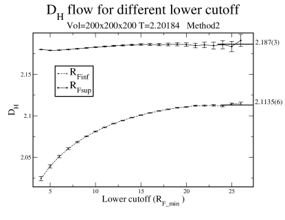
Figure 7: Dependence of $D_{H-}$ and $D_{H+}$ on the lower cutoff ($R_{F}$). The deviation between the two values is still too large even in the long-loop regime. The finale value of $D_{H}$=2.14(7) is obtained averaging over the final values for $D_{H}^{-}$ and $D_{H}^{+}$

IV.3 Method3

We finally turn to the last method ($\tt{Method3}$ below) which will prove to be the best one to extract a precise value for $D_{H}$.

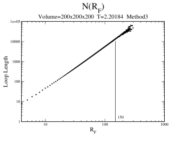
Figure 8: Loop length $N(R_{F})$ as a function of the characteristic size $R_{F}$. The best fit has been performed on the points between $4\leq R_{F}\leq 150$, to be compared with that of $\tt{Method1}$, in Fig.5.

In contrast to what is the case for Method1 and Method2, in Method3 there is no constraint on the proportions of the box containing the loops, since it is based on the approximation that, considering a large number of configuration, the different values for $D_{H}$ will eventually compensate. As can be seen from Fig.9, this method gives much better statistics both in the small- and large-loop regimes. Moreover, the longer loops considered in the statistic, having a linear dimension of $\sim 150$ (cf. Fig.8), although greater than the one considered with $\tt{Method1}$ and $\tt{Method2}$, is still smaller then the linear dimension of the lattice. Hence, finite size effects should not substantially influence the final value of $D_{H}$ obtained.

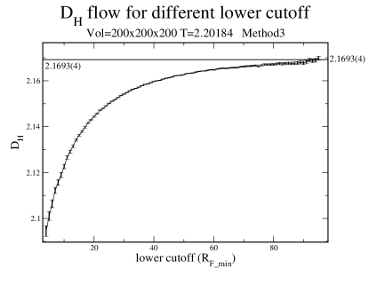
Figure 9: Dependence of $D_{H}$ on the lower cutoff ($R_{F\_min}$). The saturation region is, as can be seen, much clearer compared with previous methods. The finale value of $D_{H}=2.1693(4)$ is obtained using a weighted fit over the last three points

V Conclusions

The results obtained for the different methods are summarized in Tab.1.

All methods are in agreement with Eq.(17) and consistent with each other, although they have different accuracies. As predicted by ref.string_statistic , finite size effects are present both in the short and long-loops regime (Fig.4), but there is a clear monotonic behavior towards the continuum limit (Figs.6,7 and 9). The best results are obtained from Method 3, which yields a final value for the anomalous dimension of the condensate $\eta_{\phi}=-0.1693(4)$. This is consistent with both perturbative renormalization group calculations Folk ; Herbut ; Kang ; Halperin and previous simulations Hove_Sudbo ; Nguyen_alpha_determination ; Hove_Mo_Sudbo .

In ordinary local quantum field theories without gauge fields, one can prove that $\eta_{\phi}$ must be greater or equal to zero. In contrast, in gauge theories the proof of a non-negative $\eta_{\phi}$ is not applicable due to the non gauge-invariant form of the correlation function Nogueira ; Kleinert_1 ; Kleinert_2 . Moreover, a negative value of $\eta_{\phi}$ implies a fractal dimension larger than that of Brownian random walks, which means that the current lines are self-seeking. This point has been thoroughly discussed in Hove_Mo_Sudbo . Indeed a $D_{H}>2$ (corresponding to $\eta_{\phi}<0$) is necessary for the possibility of the existence of a phase transition driven by a vortex-loop unbinding even in the presence of a finite external magnetic field Nguyen ; Tesanovic_blow_out . This value is different from the one obtained for the 3DXY model, showing that the gauge fluctuations of the Abelian Ginzburg-Landau model (dual $3DXY$) modify the critical behavior, so that the Abelian gauge model and the $\phi^{4}$ model belong to two different universality classes.

Table 1: Values of $\tau$ and $D_{H}$, it can be seen that Eq.(17) is satisfied for all methods, and that all the values of $D_{H}$ extracted are consistent with each other. The last two columns are a check of internal consistency.

	$D_{H}$	$\tau$	$\eta_{\phi}=2-\frac{d}{\tau-1}$	$\eta_{\phi}=2-D_{H}$
$\tt{Method1}$	$2.168(6)$	2.3876(8)	-0.162(1)	-0.168(6)
$\tt{Method2}$	$2.14(7)$	2.3876(8)	-0.162(1)	-0.14(7)
$\tt{Method3}$	$2.1693(4)$	2.3876(8)	-0.162(1)	-0.1693(4)

Appendix A Vortex loops and Eq. (10)

The quantity

$$\lim_{r\to 0}F\left(\frac{|r|}{\bar{\xi}}\right)=\lim_{z\to 0}F(z)=z^{\vartheta}\qquad\vartheta>0$$ (28)

is a scaling function for the probability of traversing the distance between two points along a continuous vortex path, and holds for an ensemble of both closed and open self-avoiding walks Gennes_polimeri . Eq.(28) is often used in polymer physics to describe the statistical properties of polymer tangles. The statement that $\vartheta>0$ is certainly not true for the statistical properties of vortex loops, which are, by construction, closed and not self avoiding, so we have $P(x,x,\bar{N})\neq 0$ and $\vartheta=0$ ReplyHove . The main physical difference between vortex loops in a superconductor and a tangle of polymers, is that while polymers can start and end inside a system, this is not so for vortex loops. They must either close on themselves or alternatively thread the entire system. If we denote by ${\bf n}$ the local vorticity arising from transverse phase fluctuations, defined by Eq. (2), then we have the constraint ${\bf\nabla}\cdot{\bf n}=0$ everywhere inside the superfluid (and superconductor). We reemphasize that this in particular means that each and every vortex path in the system must be part of a closed vortex loop. No paths of vortices can be open-ended. Hence, for the former we can have $\vartheta>0$ while for the latter $\vartheta=0$. To emphasize this further, let us consider the physical meaning of a positive $\vartheta$ Janke . In the problem of self-avoiding walks, $\vartheta>0$ is an exponent that governs the asymptotic number of open-ended paths of length $N$ at the critical point, via the relation $z_{N}\sim N^{\vartheta/D_{H}}$. We also emphasize that in this paper and in previous works, we have Nguyen ; Nguyen_alpha_determination ; Hove_Sudbo exclusively been dealing with the geometrical properties of vortex-loop paths at the critical point in superfluids and superconductors.

Let us also make another remark which is relevant in this context. It is known Book_Kleinert , that the partition function of the $3DXY$ model may be expanded in so-called high-temperature (HT) graphs, which are isomorphic to the vortex-loop gas of a superconductor. In the case of charged superconductor the fluctuating gauge field screens the Coulomb interactions, and the resulting loop interactions are short rangeHove_Sudbo . Hence, for the purposes of studying the critical thermodynamics of a superconductor, one might as well use such a HT expansion of the partition function, instead of summing over all configurations of closed vortex loops of the system. In other words, at the level of the partition function, one can elevate the HT graphs to objects that are equivalent to real physical topological defects in the superconducting order parameter, i.e. closed vortex loops. A similar property is known for the two-dimensional Ising model, where one at the level of the partition function can proceed with a HT expansion and identify a formal equivalence between the closed HT graphs and the topological defects of the theory, namely closed lines in a $2D$ plane connecting domains of oppositely directed Ising spins.

However, when we compute correlation functions, as we need to do for computing the probabilities we have discussed above, the connection between physical closed vortex loop paths and the graphs of the HT expansion for the correlation functions, is far less obvious. When one utilizes the HT expansion to compute the correlation function $\langle\phi(\textbf{x})\phi^{{\dagger}}(\textbf{y})\rangle$, one has to consider open-ended graphs starting at ${\bf x}$ and ending at ${\bf y}$ Janke . One may, if one wishes, define a closed such path as the path at which the endpoint of the walk for the first time reaches a lattice point which is the nearest neighbor of the starting point, see for instance Fig. 1 of Janke . One may further go on to discuss the geometrical properties of such open-ended (and “closed”) HT graphs involved in computing the two-point correlation function in a HT expansion. However, the graphs that one then ends up with studying, have nothing to with the closed vortex paths that are the topological defects of the superconductor, and which were the objects under consideration in our previous work Hove_Sudbo . (The fractal structure of HT graphs in $O(N)$ models in two spatial dimensions, as well as the fractal structure of spin clusters and domain walls in the two-dimensional Ising model, has recently been investigated in detail Janke_PRL2005 ; Janke_PRB2005 .) The Hausdorff dimension of suchcorrelation function HT graphs will not be the same as the Hausdorff dimension of the closed vortex loops of a superconductor. Such open-ended graphs violate the constraint that the vortex-loop paths must respect, namely that they must form continuous closed paths and cannot start or end inside the system.

References

- (1) P. W. Anderson, Basic Notions in Condensed Matter (Addison-Wesley, Redwood City, California, 1984).
- (2) Z. Tesanović, Phys. Rev. B 59, 6449 (1999).
- (3) A. K. Nguyen and A. Sudbø, Euro. Phys. Lett. 46, 780 (1999).
- (4) A. K. Nguyen and A. Sudbø, Phys. Rev. B 60, 15307 (1999).
- (5) J. Hove and A. Sudbø, Phys. Rev. Lett. 84, 3426 (2000).
- (6) S. Mo, J. Hove, and A. Sudbø, Phys. Rev. B 65, (2002).
- (7) M. Peskin, Ann. Phys. (N.Y.) (1978).
- (8) S. Mo, J. Hove, and A. Sudbø, Phys. Rev. Lett. 85, 2368 (2000).
- (9) M. E. Fisher, Rep. Prog. Phys. 30, 615 (1967).
- (10) D. Stauffer and A. Aharony, Introduction to Percolation Theory (Taylor & Francis, London, new Fetter Lane 11, 1991).
- (11) C. M. Fortuin and P .W. Kasteleyn, Physica 57, 536 (1972).
- (12) B. B. Mandelbrot, The Fractal Geometry of Nature (Freeman, San Francisco,California, 1982).
- (13) N. V. Prokof’ev and B. V. Svistunov, Physics Review Letters 96, 219701 (2006).
- (14) W. Janke and A. M. J. Schakel, cond-mat/0508734 (unpublished).
- (15) C. D. Lorenz and R. M. Ziff, Phys. Rev. E 57, 230 (1998).
- (16) J. Hoshen and R. Kopelman, Phys. Rev. B 14, 3438 (1976).
- (17) M. B. Isichenko, Rev. Mod. Phys. 64, 961 (1992).
- (18) Y.-H. Li and S. Teitel, Phys. Rev. B 40, 9122 (1989).
- (19) D. Austin, E. J. Copeland, and R. J. Rivers, Phys. Rev. D 49, 4089 (1994).
- (20) R. Folk and Yu. Holovatch, J. Phys. A 29, 3409 (1996).
- (21) I. F. Herbut and Z. Tesanović, Phys. Rev. Lett. 76, 4588 (1996).
- (22) J. S. Kang, Phys. Rev. D 10, 3455 (1974).
- (23) B. I. Halperin, T. C. Lubensky, and S. K. Ma, Phys. Rev. Lett. 32, 292 (1974).
- (24) F. S. Nogueira, Phys. Rev. B 62, 14559 (2000).
- (25) H. Kleinert and F.S.Nogueira, Nucl. Phys B 651, 361 (2003).
- (26) H. Kleinert and A. M. J. Schakel, Phys. Rev. Lett. 90, 97001 (2003).
- (27) P. G. de Gennes, Scaling Concepts in Polymer physics (Cornell University Press, London, 1979), Chap. I.
- (28) J. Hove and A. Sudbo, Physics Review Letters 96, 219702 (2006).
- (29) H. Kleinert, Gauge Fields in Condensed Matter (World Scientific, Singapore, 1989), Vol. 1. Superflow and Vortex Lines.
- (30) W. Janke and A. M. J. Schakel, Phys. Rev. Lett. 95, 135702 (2005).
- (31) W. Janke and A. M. J. Schakel, Phys. Rev. E 71, 036703 (2005).