Test of a universality ansatz for the contact values of the radial distribution functions of hard-sphere mixtures near a hard wall

Abstract

Recent Monte Carlo simulation results for the contact values of polydisperse hard-sphere mixtures at a hard planar wall are considered in the light of a universality assumption made in approximate theoretical approaches. It is found that the data seem to fulfill the universality ansatz reasonably well, thus opening up the possibility of inferring properties of complicated systems from the study of simpler ones.

1 Introduction

In hard-sphere systems, the general statistical mechanical relation between the thermodynamic properties and the structural properties takes a rather simple form. Since the internal energy in these system reduces to the one of the ideal gas and the pressure equation only involves the contact values of the radial distribution functions (rdf), a knowledge of such contact values is enough to obtain their equation of state (EOS) and all their thermodynamic properties. However, such a program can not be carried out analytically due to the lack of exact expressions for these contact values up to the present day. Under these circumstances, the best one can do is to rely on sensible (approximate) proposals based on as sound as possible theoretical results or to rely on computer simulation values. Clearly, the situation is rather more complicated for mixtures than for a single component fluid and in fact for this latter many accurate (albeit empirical) equations of state have appeared in the literature from which the contact value may be readily derived.

A key analytical result is due to Lebowitz [1], who obtained the exact solution of the Percus–Yevick (PY) equation of additive hard-sphere mixtures and provided explicit expressions for the contact values of the rdf. Also analytical are the contact values of the Scaled Particle Theory (SPT) [2, 3]. Neither the PY nor the SPT lead to accurate values and so Boublík [4] (and, independently, Grundke and Henderson [5] and Lee and Levesque [6]) proposed an interpolation between the PY and the SPT contact values, that we will refer to as the BGHLL contact values, which leads to the widely used and rather accurate Boublík–Mansoori–Carnahan–Starling–Leland (BMCSL) EOS [4, 7] for hard-sphere mixtures. Refinements of the BGHLL values have been subsequently introduced, among others, by Henderson et al. [8], Matyushov and Ladanyi [9] and Barrio and Solana [10] to eliminate some drawbacks of the BMCSL EOS in the so-called colloidal limit of binary hard-sphere mixtures. On a different path but also having to do with the colloidal limit, Viduna and Smith [11] have proposed a method to obtain contact values of the rdf of hard-sphere mixtures from a given EOS. In previous work we have made proposals for the contact values of the rdf valid for mixtures with an arbitrary number of components and in arbitrary dimensionality [12, 13] and for a hard-sphere polydisperse fluid [14], that require as the only input the EOS of the one-component fluid. Apart from satisfying known consistency conditions, they are sufficiently general and flexible to accommodate any given EOS for the one-component fluid. As far as computer simulation results are concerned, contact values of the rdf of hard-sphere systems have been reported by Lee and Levesque [6], Barošová et al. [15], Lue and Woodcock [16], Cao et al. [17], Henderson et al. [18], Buzzacchi et al. [19] and Malijevský [20]. In particular, these last two references study hard-sphere mixtures in the presence of a hard planar wall.

It is interesting to point out that in the case of multicomponent mixtures of hard spheres and in the polydisperse hard-sphere fluid, the contact values which follow from the solution of the PY equation [1], those of the SPT approximation [2, 3], those of the BGHLL interpolation [4, 5, 6] and our own prescriptions [12, 13, 14] exhibit a feature that one might catalogue as a “universal” behavior because, once the packing fraction is fixed, the expressions for the contact values of the rdf for all pairs of like and unlike species depend on the diameters of both species and on the size distribution only through a single dimensionless parameter, irrespective of the number of components in the mixture.

In Ref. [14] we have presented a comparison of the different theoretical proposals for the contact values of the rdf and the ensuing EOS stemming from them with the simulation results. The aim of the present paper is to assess, apart from the accuracy of such proposals, whether the universality feature alluded to above is indeed present in the simulation data in the case of mixtures in the presence of a hard wall. This represents an extreme case and therefore a proper test ground for our approach.

The paper is organized as follows. In order to make the paper self-contained, in Sec. 2 we rederive our most recent proposal [14] for the contact values of the rdf (labelled as e3 for the reasons explained below) using some known consistency conditions and two different routes to compute the compressibility factor of a polydisperse hard-sphere system in the presence of a hard planar wall. We also point out in this section that the other proposals sharing the universality feature, namely the PY, SPT, BGHLL and our two previous proposals [12, 13] may be cast in the same form as our e3 proposal, but that only the SPT and the e3 proposals are consistent in the sense that they lead to the same compressibility factors with the two different routes. Section 3 deals with the comparison between the various contact values and simulation results, examining both the accuracy of the theories as well as whether the universality ansatz is confirmed by the simulation data. We close the paper in Sec. 4 with further discussion and some concluding remarks.

2 Contact values of the radial distribution functions

Consider a polydisperse hard-sphere mixture with a given size distribution $f(\sigma)$ (either continuous or discrete) at a given packing fraction $\eta=\frac{\pi}{6}\rho\mu_{3}$, where $\rho$ is the (total) number density and

$$\mu_{n}\equiv\langle\sigma^{n}\rangle=\int_{0}^{\infty}d\sigma\,\sigma^{n}f(\sigma)$$ (1)

is the $n$-th moment of the size distribution. Let $g(\sigma,\sigma^{\prime})$ denote the contact value of the pair correlation function of particles of diameters $\sigma$ and $\sigma^{\prime}$. This function enters into the virial expression of the EOS as [21]

$$Z\equiv\frac{p}{\rho k_{B}T} = 1+4\frac{\eta}{\mu_{3}}\int_{0}^{\infty}d\sigma\int_{0}^{\infty}d\sigma^{\prime}\,f(\sigma)f(\sigma^{\prime})\left(\frac{\sigma+\sigma^{\prime}}{2}\right)^{3}g(\sigma,\sigma^{\prime})$$ (2)

$$= 1+\frac{\eta}{2\mu_{3}}\left\langle\left(\sigma+\sigma^{\prime}\right)^{3}g(\sigma,\sigma^{\prime})\right\rangle,$$

where $Z$ is the compressibility factor, $p$ is the pressure, $k_{B}$ is the Boltzmann constant and $T$ is the absolute temperature. Assume further that the polydisperse hard-sphere mixture may find itself in the presence of a hard wall. Since a hard wall can be seen as a sphere of infinite diameter, the contact value of the correlation function $g_{w}(\sigma)$ of a sphere of diameter $\sigma$ with the wall is obtained from $g(\sigma,\sigma^{\prime})$ as

$$g_{w}(\sigma)=\lim_{\sigma^{\prime}\to\infty}g(\sigma,\sigma^{\prime}).$$ (3)

Note that $g_{w}(\sigma)=\rho_{w}(\sigma)/\rho_{\text{bulk}}(\sigma)$ provides the ratio between the density of particles of size $\sigma$ adjacent to the wall, $\rho_{w}(\sigma)$, and the density of those particles far away from the wall, $\rho_{\text{bulk}}(\sigma)$. There is a sum rule connecting the pressure and the above contact values [22], which provides an alternative route to the EOS, namely

$$Z_{w}=\int_{0}^{\infty}d\sigma\,f(\sigma)g_{w}(\sigma)=\langle g_{w}(\sigma)\rangle,$$ (4)

where the subscript $w$ in $Z_{w}$ has been used to emphasize that Eq. (4) represents a route alternative to the virial one, Eq. (2), to get the EOS of the hard-sphere polydisperse fluid. Our problem is then to compute $g(\sigma,\sigma^{\prime})$ and the associated $g_{w}(\sigma)$ for the polydisperse hard-sphere mixture in the presence of a hard wall, so that the condition $Z=Z_{w}$ is satisfied.

We consider a class of approximations of the type [13, 14]

$$g(\sigma,\sigma^{\prime})=G(z(\sigma,\sigma^{\prime})),$$ (5)

where

$$z(\sigma,\sigma^{\prime})\equiv\frac{2\sigma\sigma^{\prime}}{\sigma+\sigma^{\prime}}\frac{\mu_{2}}{\mu_{3}}$$ (6)

is a dimensionless parameter. Therefore, at a given packing fraction $\eta$, we are assuming that all the dependence of $g(\sigma,\sigma^{\prime})$ on $\sigma$, $\sigma^{\prime}$ and on the details of the size distribution $f(\sigma)$ is through the single parameter $z(\sigma,\sigma^{\prime})$. This implies that if two different pairs $(\sigma_{A},\sigma_{A}^{\prime})$ and $(\sigma_{B},\sigma_{B}^{\prime})$ in two different mixtures A and B (at the same packing fraction) have the same value of the parameter $z$, i.e., $z_{A}(\sigma_{A},\sigma_{A}^{\prime})=z_{B}(\sigma_{B},\sigma_{B}^{\prime})$, then they also have the same contact value of the rdf, i.e., $g_{A}(\sigma_{A},\sigma_{A}^{\prime})=g_{B}(\sigma_{B},\sigma_{B}^{\prime})$. The parameter $z^{-1}(\sigma,\sigma^{\prime})=(\sigma^{-1}+{\sigma^{\prime}}^{-1})/(2\mu_{2}/\mu_{3})$ can be interpreted as the arithmetic mean curvature, in appropriate units, of spheres $\sigma$ and $\sigma^{\prime}$ [13].

Notice that Eq. (5) implies in particular that $g_{w}(\sigma)=G(z_{w}(\sigma))$, where $z_{w}(\sigma)=2\sigma{\mu_{2}}/{\mu_{3}}$. Once one accepts the “universality” ansatz (5), the remaining problem lies in determining the form of the function $G(z)$. This may be achieved by considering some consistency conditions. Note that in the one-component limit, i.e., $f(\sigma)=\delta(\sigma-\sigma_{0})$, one has $z=1$, so that [12, 13]

$$G(z=1)=g_{\text{p}},$$ (7)

where $g_{\text{p}}$ is the contact value of the radial distribution function of the one-component fluid at the same packing fraction $\eta$ as the packing fraction of the mixture. Next, the case of a mixture in which one of the species is made of point particles, i.e., $\sigma\to 0$, leads to [12, 13, 14]

$$G(z=0)=\frac{1}{1-\eta}\equiv G_{0}.$$ (8)

We now want consistency between both routes to the EOS for any distribution $f(\sigma)$. To this end, we assume that $z=0$ is a regular point, take into account condition (8) and expand $G(z)$ in a power series in $z$:

$$G(z)=G_{0}+\sum_{n=1}^{\infty}G_{n}z^{n}.$$ (9)

Using the ansatz (5) and Eq. (9) in Eq. (2) one gets

$$Z = 1+\eta\sum_{n=0}^{\infty}2^{n-1}G_{n}\frac{\mu_{2}^{n}}{\mu_{3}^{n+1}}\langle\sigma^{n}{\sigma^{\prime}}^{n}\left(\sigma+\sigma^{\prime}\right)^{3-n}\rangle$$ (10)

$$= G_{0}+3\eta\frac{\mu_{1}\mu_{2}}{\mu_{3}}G_{0}+\eta\sum_{n=1}^{\infty}2^{n-1}G_{n}\frac{\mu_{2}^{n}}{\mu_{3}^{n+1}}\langle\sigma^{n}{\sigma^{\prime}}^{n}\left(\sigma+\sigma^{\prime}\right)^{3-n}\rangle,$$

where in the last step we have taken into account that

$$1+\eta\frac{G_{0}}{2\mu_{3}}\langle\left(\sigma+\sigma^{\prime}\right)^{3}\rangle = 1+\eta\frac{G_{0}}{\mu_{3}}\left(\mu_{3}+3\mu_{1}\mu_{2}\right)$$ (11)

$$= G_{0}+3\eta\frac{\mu_{1}\mu_{2}}{\mu_{3}}G_{0}.$$

Analogously, Eq. (4) becomes

$$Z_{w}=G_{0}+\sum_{n=1}^{\infty}2^{n}G_{n}\frac{\mu_{2}^{n}}{\mu_{3}^{n}}\mu_{n}.$$ (12)

Notice that if the series (9) is truncated after a given order $n\geq 3$, $Z_{w}$ is given by the first $n$ moments of the size distribution only. On the other hand, $Z$ still involves an infinite number of moments if the truncation is made after $n\geq 4$ due to the presence of terms like $\langle\sigma^{4}{\sigma^{\prime}}^{4}/(\sigma+\sigma^{\prime})\rangle$ in Eq. (10). Therefore, if we want the consistency condition $Z=Z_{w}$ to be satisfied for any polydisperse mixture, either the infinite series (9) needs to be considered or it must be truncated after $n=3$. The latter is of course the simplest possibility and thus we consider the approximation

$$G(z)=G_{0}+G_{1}z+G_{2}z^{2}+G_{3}z^{3}.$$ (13)

As a consequence, $Z$ and $Z_{w}$ depend functionally on $f(\sigma)$ only through the first three moments (which is in the spirit of Rosenfeld’s Fundamental Measure Theory [23]).

Using the approximation (13) in Eqs. (10) and (12) we are led to

$$Z=G_{0}+\eta\left[\frac{\mu_{1}\mu_{2}}{\mu_{3}}\left(3G_{0}+2G_{1}\right)+2\frac{\mu_{2}^{3}}{\mu_{3}^{2}}\left(G_{1}+2G_{2}+2G_{3}\right)\right],$$ (14)

$$Z_{w}=G_{0}+2\frac{\mu_{1}\mu_{2}}{\mu_{3}}G_{1}+4\frac{\mu_{2}^{3}}{\mu_{3}^{2}}\left(G_{2}+2G_{3}\right).$$ (15)

Thus far, the dependence of both $Z$ and $Z_{w}$ on the moments of $f(\sigma)$ is explicit and we only lack the packing-fraction dependence of $G_{1}$, $G_{2}$ and $G_{3}$. From Eqs. (14) and (15) it follows that the difference between $Z$ and $Z_{w}$ is given by

$$Z-Z_{w}=\frac{\mu_{1}\mu_{2}}{\mu_{3}}\left[3\eta G_{0}-2(1-\eta)G_{1}\right]+2\frac{\mu_{2}^{3}}{\mu_{3}^{2}}\left[\eta G_{1}-2(1-\eta)G_{2}-2(2-\eta)G_{3}\right].$$ (16)

Therefore, $Z=Z_{w}$ for any dispersity provided that

$$G_{1}=\frac{3\eta}{2\left(1-\eta\right)^{2}},$$ (17)

$$G_{2}=\frac{3\eta^{2}}{4\left(1-\eta\right)^{3}}-\frac{2-\eta}{1-\eta}G_{3},$$ (18)

where use has been made of the definition of $G_{0}$, Eq. (8). To close the problem, we use the equal size limit given in Eq. (7) and after a little algebra we are led to

$$G_{2}=(2-\eta)g_{\text{p}}-\frac{2+\eta^{2}/4}{\left(1-\eta\right)^{2}},$$ (19)

$$G_{3}=(1-\eta)\left(g_{\text{p}}^{\text{SPT}}-g_{\text{p}}\right),$$ (20)

where

$$g_{\text{p}}^{\text{SPT}}=\frac{1-\eta/2+\eta^{2}/4}{(1-\eta)^{3}}$$ (21)

is the contact value of the radial distribution function for a one-component fluid in the SPT. This completes our derivation of the e3 approximation leading to the two following main results for the contact values [24]:

$$g(\sigma,\sigma^{\prime}) = \frac{1}{1-\eta}+\frac{3\eta}{\left(1-\eta\right)^{2}}\frac{\mu_{2}}{\mu_{3}}\frac{\sigma\sigma^{\prime}}{\sigma+\sigma^{\prime}}+4\left[(2-\eta)g_{\text{p}}-\frac{2+\eta^{2}/4}{\left(1-\eta\right)^{2}}\right]\left(\frac{\mu_{2}}{\mu_{3}}\frac{\sigma\sigma^{\prime}}{\sigma+\sigma^{\prime}}\right)^{2}$$ (22)

$$+8(1-\eta)\left(g_{\text{p}}^{\text{SPT}}-g_{\text{p}}\right)\left(\frac{\mu_{2}}{\mu_{3}}\frac{\sigma\sigma^{\prime}}{\sigma+\sigma^{\prime}}\right)^{3},$$

$$g_{w}(\sigma) = \frac{1}{1-\eta}+\frac{3\eta}{\left(1-\eta\right)^{2}}\frac{\mu_{2}}{\mu_{3}}\sigma+4\left[(2-\eta)g_{\text{p}}-\frac{2+\eta^{2}/4}{\left(1-\eta\right)^{2}}\right]\left(\frac{\mu_{2}}{\mu_{3}}\sigma\right)^{2}$$ (23)

$$+8(1-\eta)\left(g_{\text{p}}^{\text{SPT}}-g_{\text{p}}\right)\left(\frac{\mu_{2}}{\mu_{3}}\sigma\right)^{3}.$$

The label e3 is meant to indicate that (i) the resulting contact values are an extension of the one-component contact value $g_{\text{p}}$ and that (ii) $G(z)$ is a cubic polynomial in $z$. As mentioned earlier, all the theoretical proposals that also comply with the universality ansatz (5), namely the PY, SPT, BGHLL and our two former proposals [12, 13] for the contact values of the rdf , may be written in the form of Eq. (13) with $G_{3}=0$, but only the SPT values also yield $Z=Z_{w}$ for any dispersity (see Table I in Ref. [14] for details). Note further that the practical application of Eqs. (22) and (23) needs only the specification of the size distribution $f(\sigma)$ and the choice of an approximate expression for $g_{\text{p}}$. For the latter, we will use the Carnahan–Starling EOS [25], namely

$$g_{\text{p}}^{\text{CS}}=\frac{1-\eta/2}{(1-\eta)^{3}}$$ (24)

and use the notation eCS3 to label the approximation. As for the size distribution, we will consider three cases:

1. The top-hat distribution of sizes given by

   $$f(\sigma)=\begin{cases}1/2c,&\mu_{1}(1-c)\leq\sigma\leq\mu_{1}(1+c)\\ 0,&\text{otherwise},\end{cases}$$ (25)

2. The Schulz distribution of the form

   $$f(\sigma)=\frac{q+1}{q!\mu_{1}}\left(\frac{q+1}{\mu_{1}}\sigma\right)^{q}\exp\left(-\frac{q+1}{\mu_{1}}\sigma\right)$$ (26)

3. The case of a bidisperse mixture, namely

   $$f(\sigma)=x_{1}\delta(\sigma-\sigma_{1})+x_{2}\delta(\sigma-\sigma_{2}),\quad x_{1}=1-x_{2}.$$ (27)

This choice of size distributions may seem to be to some extent arbitrary (one could for instance have also included a log-normal distribution). It has been mainly motivated by our desire to compare with the (to our knowledge) available simulation data for polydisperse hard-sphere mixtures in the presence of a hard planar wall. Moreover, those simulations have been computed for common packing fractions in the polydisperse systems (25)–(27). In Table 2 we present the values of the parameters corresponding to the polydisperse mixtures that have been recently studied, via Monte Carlo (MC) simulations by Buzzacchi et al. [19] and the bidisperse mixtures studied also using MC simulations by Malijevský [20]. We are now in a position to assess the merits and limitations of our proposal.

Parameters of the size distributions for the examined mixtures. Type Parameters $\eta$ Top-hat $c=0.2$ 0.2 Top-hat $c=0.2$ 0.4 Top-hat $c=0.7$ 0.4 Schulz $q=5$ 0.2 Schulz $q=5$ 0.4 Bidisperse $\sigma_{2}/\sigma_{1}=3,x_{2}=0.02$ 0.206 Bidisperse $\sigma_{2}/\sigma_{1}=3,x_{2}=0.04$ 0.207 Bidisperse $\sigma_{2}/\sigma_{1}=3,x_{2}=0.06$ 0.208 Bidisperse $\sigma_{2}/\sigma_{1}=3,x_{2}=0.0193$ 0.404 Bidisperse $\sigma_{2}/\sigma_{1}=3,x_{2}=0.0358$ 0.407 Bidisperse $\sigma_{2}/\sigma_{1}=3,x_{2}=0.0621$ 0.401

3 Comparison with simulation results

In Figs. 1 and 2 we display the comparison between the results of various approximate theories for the contact values of the wall-particle correlation functions and those obtained from computer simulations for the mixtures given in Table 2 [26]. In view of the fact that our main concern is to assess the universality ansatz, we have chosen to represent the difference $g_{w}(\sigma)-g_{w}^{\text{BGHLL}}$ as a function of $z_{w}(\sigma)/2=\sigma{\mu_{2}}/{\mu_{3}}$. The figures suggest that, although the simulation data that we have examined are only a few, the universality ansatz seems to be followed by them to a large extent, thus providing an a posteriori support to the theoretical approaches that have this feature. In particular, the data corresponding to the several polydisperse and bidisperse mixtures with $\sigma\mu_{2}/\mu_{3}\lesssim 1.5$ overlap reasonably well. In addition, the isolated points corresponding to the data for the big spheres in the bidisperse mixtures are consistent with the trend shown by the points with $\sigma\mu_{2}/\mu_{3}\lesssim 1.5$. Of course more simulations for other values of $\sigma\mu_{2}/\mu_{3}$, especially in the region $\sigma\mu_{2}/\mu_{3}\gtrsim 1.5$ or including ternary systems with higher diameter ratios (which would offer a more stringent test at higher values of $z$), would be welcome to further confirm this assertion.

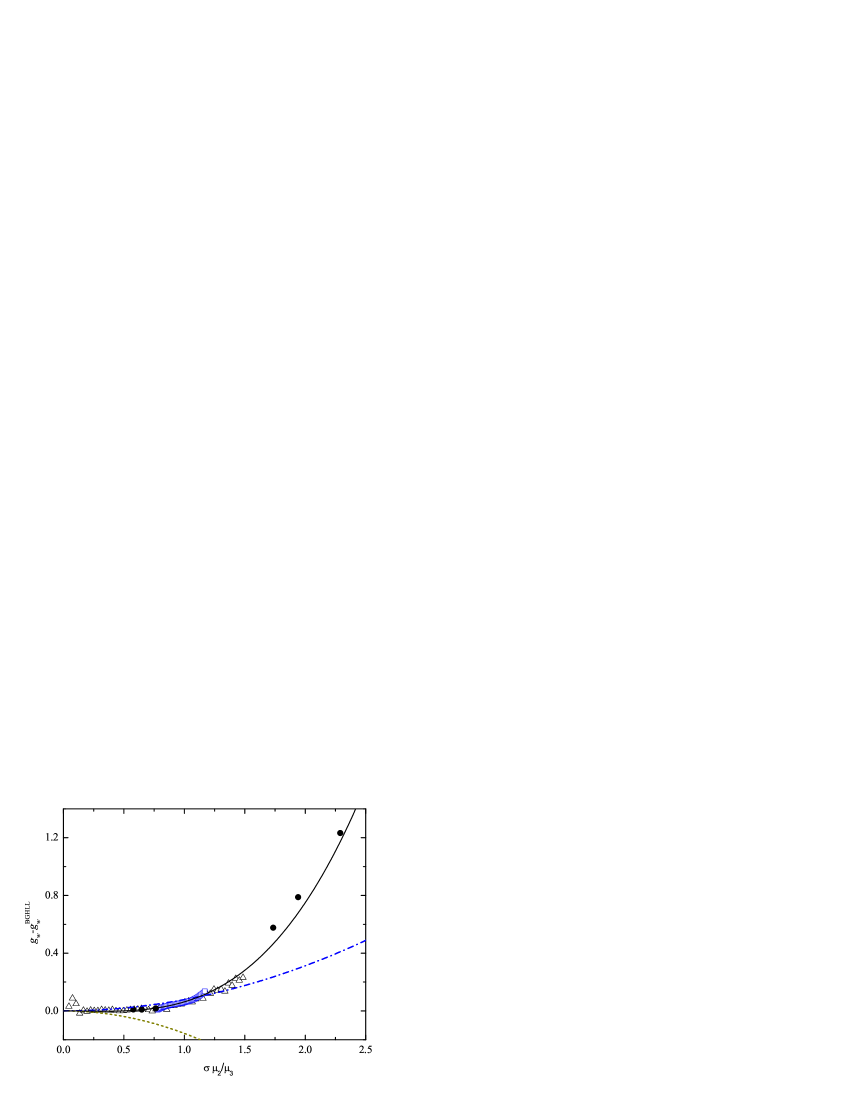
Figure 1: Plot of the difference of contact values $g_{w}-g_{w}^{\text{BGHLL}}$ as a function of $\sigma{\mu_{2}}/{\mu_{3}}$ for the different polydisperse mixtures at the fixed packing fraction $\eta=0.2$. The symbols are MC simulations: top-hat distribution with $c=0.2$ (Ref. [19]) (squares), Schulz distribution with $q=5$ (Ref. [19]) (triangles), bidisperse mixtures (Ref. [20]) (filled circles). The lines are PY(- - -), SPT (— $\cdot$ — $\cdot$) and eCS3 (—).

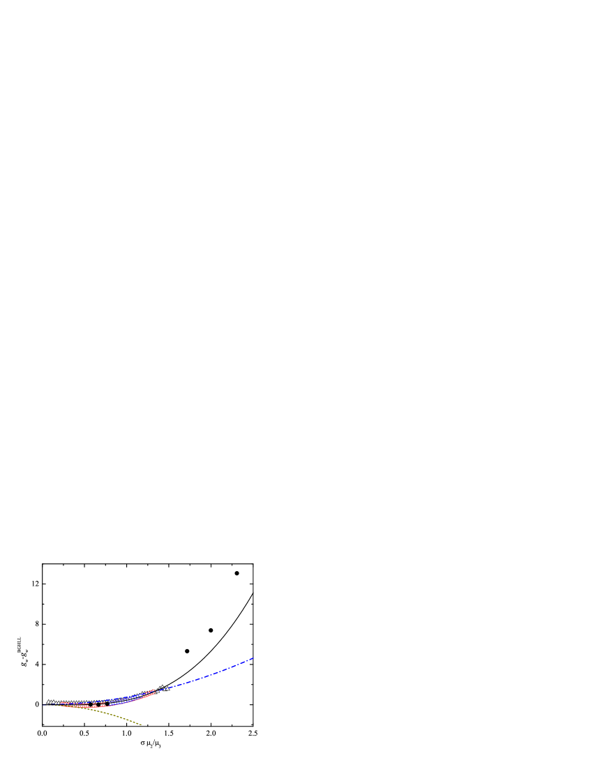
Figure 2: Plot of the difference of contact values $g_{w}-g_{w}^{\text{BGHLL}}$ as a function of $\sigma{\mu_{2}}/{\mu_{3}}$ for the different polydisperse mixtures at the fixed packing fraction $\eta=0.4$. The symbols are MC simulations: top-hat distribution with $c=0.2$ (Ref. [19]) (squares), top-hat distribution with $c=0.7$ (Ref. [19]) (circles), Schulz distribution with $q=5$ (Ref. [19]) (triangles), bidisperse mixtures (Ref. [20]) (filled circles). The lines are PY(- - -), SPT (— $\cdot$ — $\cdot$) and eCS3 (—).

Regarding the theoretical approaches, as clearly seen in the figures and already mentioned in Ref. [14], the overall trend is captured best by the eCS3 approach, while the PY approximation values are even qualitatively at odds with the simulation data. The SPT overestimates the contact values in the region $\sigma\mu_{2}/\mu_{3}\lesssim 1$ but it becomes the second best approximation for larger values of $\sigma\mu_{2}/\mu_{3}$. In the latter region, all the theories underestimate the simulation data, the eCS3 predictions being the most accurate, especially for the smallest packing fraction.

4 Concluding remarks

In this paper we have examined the universality assumption that is present in many theoretical derivations by which, once the packing fraction is fixed, for all pairs of like and unlike spheres in a polydisperse hard-sphere mixture with an arbitrary size distribution and in the presence of a hard wall, the dependence of the contact values of the particle-particle correlation function, $g(\sigma,\sigma^{\prime})$, and of the wall-particle correlation function, $g_{w}(\sigma)$, on the diameters and on the composition is only through a single dimensionless parameter and holds for an arbitrary number of components. This was done by comparison with available MC simulation results for $g_{w}(\sigma)$ because, since $z_{w}(\sigma)>z(\sigma,\sigma^{\prime})$, these contact values represent a more stringent test for the universality ansatz than the values of $g(\sigma,\sigma^{\prime})$. While our analysis is limited due to the few data that are at hand, the results suggest that indeed the simulation data seem to comply reasonably well with the ansatz, the results corresponding to the three different bidisperse mixtures virtually falling on top of the polydisperse ones for common values of $z_{w}$. The results also indicate that our eCS3 approximation does a rather reasonable job. Although it underestimates the simulation data for high values of the parameter $z_{w}$, it is still better than the other approximations sharing the same universality property.

A noteworthy aspect of the comparison between the simulation data and the theoretical approximations is that those proposals that fulfill the condition $Z=Z_{w}$, namely the SPT and eCS3, are the ones that show the best performance for high $z_{w}$. Since, as shown by Eq. (20) and discussed in Ref. [14], our e3 approach becomes identical to the SPT one when the choice $g_{\text{p}}=g_{\text{p}}^{\text{SPT}}$ instead of $g_{\text{p}}=g_{\text{p}}^{\text{CS}}$ is made, we can interpret it as a versatile and flexible generalization of SPT. We are fully aware that, apart from the consistency conditions that we have used, there exist extra ones (see for instance Ref. [27]) that one might use as well within our approach. Assuming that the ansatz (5) still holds, these conditions are related to the derivatives of $G$ with respect to $z$, namely

$$\left.\frac{\partial G(z)}{\partial z}\right|_{z=0}=\frac{3\eta}{2(1-\eta)^{2}},$$ (28)

$$\left.\frac{\partial^{2}G(z)}{\partial z^{2}}\right|_{z=0}=\frac{3\eta}{1-\eta}\left(g_{\text{PY}}-\frac{1}{2}g\right),$$ (29)

$$\left.\frac{\partial^{3}G(z)}{\partial z^{3}}\right|_{z=2}=0,$$ (30)

where $g_{\text{p}}^{\text{PY}}=(1+\eta/2)/(1-\eta)^{2}$ is the contact value of the one-component hard-sphere fluid in the PY approximation. The question immediately arises as to whether the fulfillment of these extra conditions might influence the results we have presented in this paper. Interestingly enough, as shown by Eq. (17), condition (28) is already satisfied by our e3 approximation without having to be imposed. On the other hand, condition (30) implies $G_{3}=0$ in the e3 scheme and thus it is only satisfied if $g_{\text{p}}=g_{\text{p}}^{\text{SPT}}$, in which case we recover the SPT. Condition (29) is not fulfilled either by the SPT or by the e3 approximation (except for a particular expression of $g_{\text{p}}$ which is otherwise not very accurate). Thus, fulfilling the extra conditions (29) and (30) with a free $g_{\text{p}}$ requires either considering a higher order polynomial in $z$ (in which case the consistency condition $Z=Z_{w}$ cannot be satisfied for arbitrary mixtures, as discussed before) or not using the universality ansatz at all. In the first case, we have checked that a quartic or even a quintic polynomial does not improve matters, whereas giving up the universality assumption increases significantly the number of parameters to be determined and seems not to be adequate in view of the behavior observed in the simulation data. Therefore, e3 appears to be a very reasonable compromise between simplicity and accuracy, with the added bonus of being versatile to accommodate any choice for $g_{\text{p}}$.

Finally, one should point out that the fact that the simulation results give support to the validity of the universality assumption, opens up the possibility of gaining information of rather complicated polydisperse mixtures from the knowledge of simpler systems using an approximation like our e3 approximation.

We want to thank Dr. Alexandr Malijevský for making his simulation results available to us prior to publication and Dr. David Reguera for bringing Ref. [27] to our attention. M.L.H. acknowledges the financial support of DGAPA-UNAM under project IN-110406. The research of A.S. and S.B.Y. has also been supported by the Ministerio de Educación y Ciencia (Spain) through grant No. FIS2004-01399 (partially financed by FEDER funds).

References

- [1] J. L. Lebowitz, Phys. Rev. A 133, 895 (1964).
- [2] H. Reiss, H. L. Frisch and J. L. Lebowitz, J. Chem. Phys. 31, 389 (1959); J. L. Lebowitz, E. Helfand and E. Praestgaard, J. Chem. Phys. 43, 774 (1965); M. J. Mandell and H. Reiss, J. Stat. Phys. 13, 113 (1975).
- [3] Y. Rosenfeld, J. Chem. Phys. 89, 4272 (1988).
- [4] T. Boublík, J. Chem. Phys. 53, 471 (1970).
- [5] E. W. Grundke and D. Henderson, Mol. Phys. 24, 269 (1972).
- [6] L. L. Lee and D. Levesque, Mol. Phys. 26, 1351 (1973).
- [7] G. A. Mansoori, N. F. Carnahan, K. E. Starling and J. T. W. Leland, J. Chem. Phys. 54, 1523 (1971).
- [8] D. Henderson, A. Malijevský, S. Labík and K.-Y. Chan, Mol. Phys. 87, 273 (1996); D. H. L. Yau, K.-Y. Chan and D. Henderson, ibid. 88, 1237 (1996); 91, 1813 (1997); D. Henderson and K.-Y. Chan, J. Chem. Phys. 108, 9946 (1998); Mol. Phys. 94, 253 (1998); D. Matyushov, D. Henderson and K.-Y. Chan, ibid. 96, 1813 (1999); D. Henderson and K.-Y. Chan, ibid. 98, 1005 (2000).
- [9] D. V. Matyushov and B. M. Ladanyi, J. Chem. Phys. 107, 5815 (1997)
- [10] C. Barrio and J. R. Solana, J. Chem. Phys. 113, 10180 (2000).
- [11] D. Viduna and W. R. Smith, Mol. Phys. 100, 2903 (2002); J. Chem. Phys. 117, 1214 (2002).
- [12] A. Santos, S. B. Yuste and M. López de Haro, Mol. Phys. 96, 1 (1999).
- [13] A. Santos, S. B. Yuste and M. López de Haro, J. Chem. Phys. 117, 5785 (2002).
- [14] A. Santos, S. B. Yuste and M. López de Haro, J. Chem. Phys. 123, 234512 (2005).
- [15] M. Barošová, A. Malijevský, S. Labík and W. R. Smith, Mol. Phys. 87, 423 (1996)
- [16] L. Lue and L. V. Woodcock, Mol. Phys. 96, 1435 (1999).
- [17] D. Cao, K.-Y. Chan, D. Henderson and W. Wang, Mol. Phys. 98, 619 (2000).
- [18] D. Henderson, A. Trokhymchuk, L. V. Woodcock and K.-Y. Chan, Mol. Phys. 103, 667 (2005).
- [19] M. Buzzacchi, I. Pagonabarraga and N. B. Wilding, J. Chem. Phys. 121, 11362 (2004).
- [20] Al. Malijevský, private communication.
- [21] F. Lado, Phys. Rev. E 54, 4411 (1996).
- [22] R. Evans, in Liquids and Interfaces, edited by J. Charvolin, J. F. Joanny and J. Zinn-Justin (North-Holland, Amsterdam, 1990).
- [23] Y. Rosenfeld, Phys. Rev. Lett. 63, 980 (1989).
- [24] Of course one may use these values to immediately write the compressibility factor using either Eq. (14) or Eq. (15). The corresponding expression will be ommitted since it is not required for the purposes of the present paper but may be found in Ref. [14].
- [25] N. F. Carnahan and K. E. Starling, J. Chem. Phys. 51, 635 (1969).
- [26] Notice that the actual packing fractions of the bidisperse mixtures quoted in Table 2 are rather close but not exactly and . One should expect nevertheless that these minor differences should have little influence on our analysis of the overall trends.
- [27] M. Heying and D. S. Corti, J. Phys. Chem. B, 108, 19756 (2004).